Tag Archives: machine learning

MobileDiffusion: Rapid text-to-image generation on-device

Text-to-image diffusion models have shown exceptional capabilities in generating high-quality images from text prompts. However, leading models feature billions of parameters and are consequently expensive to run, requiring powerful desktops or servers (e.g., Stable Diffusion, DALL·E, and Imagen). While recent advancements in inference solutions on Android via MediaPipe and iOS via Core ML have been made in the past year, rapid (sub-second) text-to-image generation on mobile devices has remained out of reach.

To that end, in “MobileDiffusion: Subsecond Text-to-Image Generation on Mobile Devices”, we introduce a novel approach with the potential for rapid text-to-image generation on-device. MobileDiffusion is an efficient latent diffusion model specifically designed for mobile devices. We also adopt DiffusionGAN to achieve one-step sampling during inference, which fine-tunes a pre-trained diffusion model while leveraging a GAN to model the denoising step. We have tested MobileDiffusion on iOS and Android premium devices, and it can run in half a second to generate a 512x512 high-quality image. Its comparably small model size of just 520M parameters makes it uniquely suited for mobile deployment.

      
Rapid text-to-image generation on-device.

Background

The relative inefficiency of text-to-image diffusion models arises from two primary challenges. First, the inherent design of diffusion models requires iterative denoising to generate images, necessitating multiple evaluations of the model. Second, the complexity of the network architecture in text-to-image diffusion models involves a substantial number of parameters, regularly reaching into the billions and resulting in computationally expensive evaluations. As a result, despite the potential benefits of deploying generative models on mobile devices, such as enhancing user experience and addressing emerging privacy concerns, it remains relatively unexplored within the current literature.

The optimization of inference efficiency in text-to-image diffusion models has been an active research area. Previous studies predominantly concentrate on addressing the first challenge, seeking to reduce the number of function evaluations (NFEs). Leveraging advanced numerical solvers (e.g., DPM) or distillation techniques (e.g., progressive distillation, consistency distillation), the number of necessary sampling steps have significantly reduced from several hundreds to single digits. Some recent techniques, like DiffusionGAN and Adversarial Diffusion Distillation, even reduce to a single necessary step.

However, on mobile devices, even a small number of evaluation steps can be slow due to the complexity of model architecture. Thus far, the architectural efficiency of text-to-image diffusion models has received comparatively less attention. A handful of earlier works briefly touches upon this matter, involving the removal of redundant neural network blocks (e.g., SnapFusion). However, these efforts lack a comprehensive analysis of each component within the model architecture, thereby falling short of providing a holistic guide for designing highly efficient architectures.


MobileDiffusion

Effectively overcoming the challenges imposed by the limited computational power of mobile devices requires an in-depth and holistic exploration of the model's architectural efficiency. In pursuit of this objective, our research undertakes a detailed examination of each constituent and computational operation within Stable Diffusion’s UNet architecture. We present a comprehensive guide for crafting highly efficient text-to-image diffusion models culminating in the MobileDiffusion.

The design of MobileDiffusion follows that of latent diffusion models. It contains three components: a text encoder, a diffusion UNet, and an image decoder. For the text encoder, we use CLIP-ViT/L14, which is a small model (125M parameters) suitable for mobile. We then turn our focus to the diffusion UNet and image decoder.


Diffusion UNet

As illustrated in the figure below, diffusion UNets commonly interleave transformer blocks and convolution blocks. We conduct a comprehensive investigation of these two fundamental building blocks. Throughout the study, we control the training pipeline (e.g., data, optimizer) to study the effects of different architectures.

In classic text-to-image diffusion models, a transformer block consists of a self-attention layer (SA) for modeling long-range dependencies among visual features, a cross-attention layer (CA) to capture interactions between text conditioning and visual features, and a feed-forward layer (FF) to post-process the output of attention layers. These transformer blocks hold a pivotal role in text-to-image diffusion models, serving as the primary components responsible for text comprehension. However, they also pose a significant efficiency challenge, given the computational expense of the attention operation, which is quadratic to the sequence length. We follow the idea of UViT architecture, which places more transformer blocks at the bottleneck of the UNet. This design choice is motivated by the fact that the attention computation is less resource-intensive at the bottleneck due to its lower dimensionality.

Our UNet architecture incorporates more transformers in the middle, and skips self-attention (SA) layers at higher resolutions.

Convolution blocks, in particular ResNet blocks, are deployed at each level of the UNet. While these blocks are instrumental for feature extraction and information flow, the associated computational costs, especially at high-resolution levels, can be substantial. One proven approach in this context is separable convolution. We observed that replacing regular convolution layers with lightweight separable convolution layers in the deeper segments of the UNet yields similar performance.

In the figure below, we compare the UNets of several diffusion models. Our MobileDiffusion exhibits superior efficiency in terms of FLOPs (floating-point operations) and number of parameters.

Comparison of some diffusion UNets.

Image decoder

In addition to the UNet, we also optimized the image decoder. We trained a variational autoencoder (VAE) to encode an RGB image to an 8-channel latent variable, with 8× smaller spatial size of the image. A latent variable can be decoded to an image and gets 8× larger in size. To further enhance efficiency, we design a lightweight decoder architecture by pruning the original’s width and depth. The resulting lightweight decoder leads to a significant performance boost, with nearly 50% latency improvement and better quality. For more details, please refer to our paper.

VAE reconstruction. Our VAE decoders have better visual quality than SD (Stable Diffusion).

Decoder   #Params (M)     PSNR↑     SSIM↑     LPIPS↓  
SD 49.5 26.7 0.76 0.037
Ours 39.3 30.0 0.83 0.032
Ours-Lite     9.8 30.2 0.84 0.032

Quality evaluation of VAE decoders. Our lite decoder is much smaller than SD, with better quality metrics, including peak signal-to-noise ratio (PSNR), structural similarity index measure (SSIM), and Learned Perceptual Image Patch Similarity (LPIPS).

One-step sampling

In addition to optimizing the model architecture, we adopt a DiffusionGAN hybrid to achieve one-step sampling. Training DiffusionGAN hybrid models for text-to-image generation encounters several intricacies. Notably, the discriminator, a classifier distinguishing real data and generated data, must make judgments based on both texture and semantics. Moreover, the cost of training text-to-image models can be extremely high, particularly in the case of GAN-based models, where the discriminator introduces additional parameters. Purely GAN-based text-to-image models (e.g., StyleGAN-T, GigaGAN) confront similar complexities, resulting in highly intricate and expensive training.

To overcome these challenges, we use a pre-trained diffusion UNet to initialize the generator and discriminator. This design enables seamless initialization with the pre-trained diffusion model. We postulate that the internal features within the diffusion model contain rich information of the intricate interplay between textual and visual data. This initialization strategy significantly streamlines the training.

The figure below illustrates the training procedure. After initialization, a noisy image is sent to the generator for one-step diffusion. The result is evaluated against ground truth with a reconstruction loss, similar to diffusion model training. We then add noise to the output and send it to the discriminator, whose result is evaluated with a GAN loss, effectively adopting the GAN to model a denoising step. By using pre-trained weights to initialize the generator and the discriminator, the training becomes a fine-tuning process, which converges in less than 10K iterations.

Illustration of DiffusionGAN fine-tuning.

Results

Below we show example images generated by our MobileDiffusion with DiffusionGAN one-step sampling. With such a compact model (520M parameters in total), MobileDiffusion can generate high-quality diverse images for various domains.

Images generated by our MobileDiffusion

We measured the performance of our MobileDiffusion on both iOS and Android devices, using different runtime optimizers. The latency numbers are reported below. We see that MobileDiffusion is very efficient and can run within half a second to generate a 512x512 image. This lightning speed potentially enables many interesting use cases on mobile devices.

Latency measurements (s) on mobile devices.

Conclusion

With superior efficiency in terms of latency and size, MobileDiffusion has the potential to be a very friendly option for mobile deployments given its capability to enable a rapid image generation experience while typing text prompts. And we will ensure any application of this technology will be in-line with Google’s responsible AI practices.


Acknowledgments

We like to thank our collaborators and contributors that helped bring MobileDiffusion to on-device: Zhisheng Xiao, Yanwu Xu, Jiuqiang Tang, Haolin Jia, Lutz Justen, Daniel Fenner, Ronald Wotzlaw, Jianing Wei, Raman Sarokin, Juhyun Lee, Andrei Kulik, Chuo-Ling Chang, and Matthias Grundmann.

Source: Google AI Blog


YouTube Ads Creative Analysis

Posted by Brian Craft, Satish Shreenivasa, Huikun Zhang, Manisha Arora and Paul Cubre – gTech Data Science Team


Introduction


Why analyze YouTube ads?

YouTube has billions of monthly logged-in users and every day people watch billions of hours of video and generate billions of views. Businesses can connect with YouTube users using YouTube ads, which are promotional videos that appear on YouTube's website and app, with a variety of video ad formats and goals.

Image of a sample YouTube in-stream skippable video ad
A sample YouTube in-stream skippable video ad

The Challenge

An effective video ad focuses on the ABCDs.

  • Attention: Capturing the viewer's attention till the end.
  • Branding: Helping them hear or visualize the brand.
  • Connection: Making them feel something about the brand.
  • Direction: Encouraging them to take action.

But each YouTube ad has a varying number of components, for instance, objects, background music or a logo. Each of these components affect the view through rate (which is referred to as VTR for the remainder of the post) of the video ad. Therefore, analyzing video ads through the lens of the components in the ad helps businesses understand what about the ad improves VTR. The insights from these analyses can be used to inform the creation of new creatives and to optimize existing creatives to improve VTR.


The Proposal

We propose a machine learning based approach for analyzing a company’s YouTube ads to assess which components affect VTR, for the purpose of optimizing a video ad’s performance. We illustrate how to:

  • Use Google Cloud Video Intelligence API to extract the components of each video ad, using the underlying video files.
  • Transform that extracted data to engineered features that map to actionable business questions.
  • Use a machine learning model to isolate the effect on VTR of each engineered feature.
  • Interpret and action on those insights to improve video ad performance, for instance altering existing creatives or create new creatives to be used in an AB test.

Approach


The Process

The proposed analysis has 5 steps, discussed below.

1. Define Business Questions
Align on a list of business questions that are actionable, for instance “does having a logo in the opening shot affect VTR?” We suggest taking feasibility into account ahead of time, for instance if a product disclaimer is necessary to have for legal reasons, there is no reason to assess the impact a disclaimer has on VTR.

2. Raw Component Extraction
Use Google Cloud technologies, such as the Google Cloud Video Intelligence API, and underlying video files to extract raw components from each video ad. For instance, but not limited to, objects appearing in the video at a particular timestamp, presence of text and its location on the screen, or the presence of specific sounds.

3. Feature Engineering
Using the raw components extracted in step 2, engineer features that align to the business questions defined in step 1. For example, if the business question is “does having a logo in the opening shot affect VTR”, create a feature that labels each video as either 1, having a logo in the opening shot or 0, not having a logo in the opening shot. Repeat this for each feature.

4. Modeling
Create an ML model using the engineered features from step 3, using VTR as the target in the model.

5. Interpretation
Extract statistically significant features from the ML model and interpret their effect on VTR. For example, “there is an xx% observed uplift in VTR when there is a logo in the opening shot.”


Feature Engineering


Data Extraction

Consider 2 different YouTube Video Ads for a web browser, each highlighting a different product feature. Ad A has text that says “Built In Virus Protection'', while Ad B has text that says “Automatic Password Saving”.

The raw text can be extracted from each video ad and allow for the creation of tabular datasets, such as the below. For brevity and simplicity, the example carried forward will deal with text features only and forgo the timestamp dimension.

 Ad

 Detected Raw Text

 Ad A

 Built In Virus Protection

 Ad B

 Automatic Password Saving


Preprocessing

After extracting the raw components in each ad, preprocessing may need to be applied, such as removing case sensitivity and punctuation.

 Ad

 Detected Raw Text

 Processed Text

 Ad A

 Built IVirus Protection

 built ivirus protection

 Ad B

 Automatic Password Saving

 automatic password saving


Manual Feature Engineering

Consider a scenario where the goal is to answer the business question, “does having a textual reference to a product feature affect VTR?”

This feature could be built manually by exploring all the text in all the videos in the sample and creating a list of tokens or phrases that indicate a textual reference to a product feature. However, this approach can be time consuming and limits scaling.

Image of pseudo code for manual feature engineering
Pseudo code for manual feature engineering

AI Based Feature Engineering

Instead of manual feature engineering as described above, the text detected in each video ad creative can be passed to an LLM along with a prompt that performs the feature engineering automatically.

For example, if the goal is to explore the value of highlighting a product feature in a video ad, ask an LLM if the text “‘built in virus protection’ is a feature callout”, followed by asking the LLM if the text “‘automatic password saving’ is a feature callout”.

The answers can be extracted and transformed to a 0 or 1, to later be passed to a machine learning model.

 Ad

 Raw Text

 Processed Text

 Has Textual Reference to Feature

 Ad A

 Built IVirus Protection

 built ivirus protection

 Yes

 Ad B

 Automatic Password Saving

 automatic password saving

 Yes


Modeling


Training Data

The result of the feature engineering step is a dataframe with columns that align to the initial business questions, which can be joined to a dataframe that has the VTR for each video ad in the sample.

 Ad

 Has Textual Reference to Feature

 VTR*

 Ad A

 Yes

 10%

 Ad B

 Yes

 50%


*Values are random and not to be interpreted in any way.

Modeling is done using fixed effects, bootstrapping and ElasticNet. More information can be found here in the post Introducing Discovery Ad Performance Analysis, written by Manisha Arora and Nithya Mahadevan.

Interpretation

The model output can be used to extract significant features, coefficient values, and standard deviation.

Coefficient Value (+/- X%)
Represents the absolute percentage uplift in VTR. Positive value indicates positive impact on VTR and a negative value indicates a negative impact on VTR.

Significant Value (True/False)
Represents whether the feature has a statistically significant impact on VTR.

 Feature

 Coefficient*

 Standard Deviation*

 Significant?*

 Has Textual Reference to Feature

0.0222

0.000033

True


*Values are random and not to be interpreted in any way.

In the above hypothetical example, the feature “Has Feature Callout” has a statistically significant, positive impact of VTR. This can be interpreted as “there is an observed 2.22% absolute uplift in VTR when an ad has a textual reference to a product feature.”

Challenges

Challenges of the above approach are:

  • Interactions among the individual features input into the model are not considered. For example, if “has logo” and “has logo in the lower left” are individual features in the model, their interaction will not be assessed. However, a third feature can be engineered combining the above as “has large logo + has logo in the lower left”.
  • Inferences are based on historical data and not necessarily representative of future ad creative performance. There is no guarantee that insights will improve VTR.
  • Dimensionality can be a concern as given the number of components in a video ad.

Activation Strategies


Ads Creative Studio

Ads Creative Studio is an effective tool for businesses to create multiple versions of a video by quickly combining text, images, video clips or audio. Use this tool to create new videos quickly by adding/removing features in accordance with model output.

Image of sample video creation features in Ads creative studio
Sample video creation features in Ads creative studio

Video Experiments

Design a new creative, varying a component based on the insights from the analysis, and run an AB test. For example, change the size of the logo and set up an experiment using Video Experiments.


Summary


Identifying which components of a YouTube Ad affect VTR is difficult, due to the number of components contained in the ad, but there is an incentive for advertisers to optimize their creatives to improve VTR. Google Cloud technologies, GenAI models and ML can be used to answer creative centric business questions in a scalable and actionable way. The resulting insights can be used to optimize YouTube ads and achieve business outcomes.


Acknowledgements

We would like to thank our collaborators at Google, specifically Luyang Yu, Vijai Kasthuri Rangan, Ahmad Emad, Chuyi Wang, Kun Chang, Mike Anderson, Yan Sun, Nithya Mahadevan, Tommy Mulc, David Letts, Tony Coconate, Akash Roy Choudhury, Alex Pronin, Toby Yang, Felix Abreu and Anthony Lui.

VideoPoet: A large language model for zero-shot video generation

A recent wave of video generation models has burst onto the scene, in many cases showcasing stunning picturesque quality. One of the current bottlenecks in video generation is in the ability to produce coherent large motions. In many cases, even the current leading models either generate small motion or, when producing larger motions, exhibit noticeable artifacts.

To explore the application of language models in video generation, we introduce VideoPoet, a large language model (LLM) that is capable of a wide variety of video generation tasks, including text-to-video, image-to-video, video stylization, video inpainting and outpainting, and video-to-audio. One notable observation is that the leading video generation models are almost exclusively diffusion-based (for one example, see Imagen Video). On the other hand, LLMs are widely recognized as the de facto standard due to their exceptional learning capabilities across various modalities, including language, code, and audio (e.g., AudioPaLM). In contrast to alternative models in this space, our approach seamlessly integrates many video generation capabilities within a single LLM, rather than relying on separately trained components that specialize on each task.


Overview

The diagram below illustrates VideoPoet’s capabilities. Input images can be animated to produce motion, and (optionally cropped or masked) video can be edited for inpainting or outpainting. For stylization, the model takes in a video representing the depth and optical flow, which represent the motion, and paints contents on top to produce the text-guided style.

An overview of VideoPoet, capable of multitasking on a variety of video-centric inputs and outputs. The LLM can optionally take text as input to guide generation for text-to-video, image-to-video, video-to-audio, stylization, and outpainting tasks. Resources used: Wikimedia Commons and DAVIS.

Language models as video generators

One key advantage of using LLMs for training is that one can reuse many of the scalable efficiency improvements that have been introduced in existing LLM training infrastructure. However, LLMs operate on discrete tokens, which can make video generation challenging. Fortunately, there exist video and audio tokenizers, which serve to encode video and audio clips as sequences of discrete tokens (i.e., integer indices), and which can also be converted back into the original representation.

VideoPoet trains an autoregressive language model to learn across video, image, audio, and text modalities through the use of multiple tokenizers (MAGVIT V2 for video and image and SoundStream for audio). Once the model generates tokens conditioned on some context, these can be converted back into a viewable representation with the tokenizer decoders.

A detailed look at the VideoPoet task design, showing the training and inference inputs and outputs of various tasks. Modalities are converted to and from tokens using tokenizer encoder and decoders. Each modality is surrounded by boundary tokens, and a task token indicates the type of task to perform.

Examples generated by VideoPoet

Some examples generated by our model are shown below.

Videos generated by VideoPoet from various text prompts. For specific text prompts refer to the website.

For text-to-video, video outputs are variable length and can apply a range of motions and styles depending on the text content. To ensure responsible practices, we reference artworks and styles in the public domain e.g., Van Gogh’s “Starry Night”.

Text Input    “A Raccoon dancing in Times Square”    “A horse galloping through Van-Gogh’s ‘Starry Night’”    “Two pandas playing cards”    “A large blob of exploding splashing rainbow paint, with an apple emerging, 8k”
Video Output            

For image-to-video, VideoPoet can take the input image and animate it with a prompt.

An example of image-to-video with text prompts to guide the motion. Each video is paired with an image to its left. Left: “A ship navigating the rough seas, thunderstorm and lightning, animated oil on canvas”. Middle: “Flying through a nebula with many twinkling stars”. Right: “A wanderer on a cliff with a cane looking down at the swirling sea fog below on a windy day”. Reference: Wikimedia Commons, public domain**.

For video stylization, we predict the optical flow and depth information before feeding into VideoPoet with some additional input text.

Examples of video stylization on top of VideoPoet text-to-video generated videos with text prompts, depth, and optical flow used as conditioning. The left video in each pair is the input video, the right is the stylized output. Left: “Wombat wearing sunglasses holding a beach ball on a sunny beach.” Middle: “Teddy bears ice skating on a crystal clear frozen lake.” Right: “A metal lion roaring in the light of a forge.”

VideoPoet is also capable of generating audio. Here we first generate 2-second clips from the model and then try to predict the audio without any text guidance. This enables generation of video and audio from a single model.


An example of video-to-audio, generating audio from a video example without any text input.

By default, the VideoPoet model generates videos in portrait orientation to tailor its output towards short-form content. To showcase its capabilities, we have produced a brief movie composed of many short clips generated by VideoPoet. For the script, we asked Bard to write a short story about a traveling raccoon with a scene-by-scene breakdown and a list of accompanying prompts. We then generated video clips for each prompt, and stitched together all resulting clips to produce the final video below.


When we developed VideoPoet, we noticed some nice properties of the model’s capabilities, which we highlight below.


Long video

We are able to generate longer videos simply by conditioning on the last 1 second of video and predicting the next 1 second. By chaining this repeatedly, we show that the model can not only extend the video well but also faithfully preserve the appearance of all objects even over several iterations.

Here are two examples of VideoPoet generating long video from text input:

Text Input    “An astronaut starts dancing on Mars. Colorful fireworks then explode in the background.”    “FPV footage of a very sharp elven city of stone in the jungle with a brilliant blue river, waterfall, and large steep vertical cliff faces.”           
Video Output                 

It is also possible to interactively edit existing video clips generated by VideoPoet. If we supply an input video, we can change the motion of objects to perform different actions. The object manipulation can be centered at the first frame or the middle frames, which allow for a high degree of editing control.

For example, we can randomly generate some clips from the input video and select the desired next clip.

An input video on the left is used as conditioning to generate four choices given the initial prompt: “Closeup of an adorable rusty broken-down steampunk robot covered in moss moist and budding vegetation, surrounded by tall grass”. For the first three outputs we show what would happen for unprompted motions. For the last video in the list below, we add to the prompt, “powering up with smoke in the background” to guide the action.

Image to video control

Similarly, we can apply motion to an input image to edit its contents towards the desired state, conditioned on a text prompt.

Animating a painting with different prompts. Left: “A woman turning to look at the camera.” Right: “A woman yawning.” **

Camera motion

We can also accurately control camera movements by appending the type of desired camera motion to the text prompt. As an example, we generated an image by our model with the prompt, “Adventure game concept art of a sunrise over a snowy mountain by a crystal clear river”. The examples below append the given text suffix to apply the desired motion.

Prompts from left to right: “Zoom out”, “Dolly zoom”, “Pan left”, “Arc shot”, “Crane shot”, “FPV drone shot”.

Evaluation results

We evaluate VideoPoet on text-to-video generation with a variety of benchmarks to compare the results to other approaches. To ensure a neutral evaluation, we ran all models on a wide variation of prompts without cherry-picking examples and asked people to rate their preferences. The figure below highlights the percentage of the time VideoPoet was chosen as the preferred option in green for the following questions.


Text fidelity

User preference ratings for text fidelity, i.e., what percentage of videos are preferred in terms of accurately following a prompt.

Motion interestingness

User preference ratings for motion interestingness, i.e., what percentage of videos are preferred in terms of producing interesting motion.

Based on the above, on average people selected 24–35% of examples from VideoPoet as following prompts better than a competing model vs. 8–11% for competing models. Raters also preferred 41–54% of examples from VideoPoet for more interesting motion than 11–21% for other models.


Conclusion

Through VideoPoet, we have demonstrated LLMs’ highly-competitive video generation quality across a wide variety of tasks, especially in producing interesting and high quality motions within videos. Our results suggest the promising potential of LLMs in the field of video generation. For future directions, our framework should be able to support “any-to-any” generation, e.g., extending to text-to-audio, audio-to-video, and video captioning should be possible, among many others.

To view more examples in original quality, see the website demo.


Acknowledgements

This research has been supported by a large body of contributors, including Dan Kondratyuk, Lijun Yu, Xiuye Gu, José Lezama, Jonathan Huang, Rachel Hornung, Hartwig Adam, Hassan Akbari, Yair Alon, Vighnesh Birodkar, Yong Cheng, Ming-Chang Chiu, Josh Dillon, Irfan Essa, Agrim Gupta, Meera Hahn, Anja Hauth, David Hendon, Alonso Martinez, David Minnen, David Ross, Grant Schindler, Mikhail Sirotenko, Kihyuk Sohn, Krishna Somandepalli, Huisheng Wang, Jimmy Yan, Ming-Hsuan Yang, Xuan Yang, Bryan Seybold, and Lu Jiang.

We give special thanks to Alex Siegman and Victor Gomes for managing computing resources. We also give thanks to Aren Jansen, Marco Tagliasacchi, Neil Zeghidour, John Hershey for audio tokenization and processing, Angad Singh for storyboarding in “Rookie the Raccoon”, Cordelia Schmid for research discussions, Alonso Martinez for graphic design, David Salesin, Tomas Izo, and Rahul Sukthankar for their support, and Jay Yagnik as architect of the initial concept.


**
(a) The Storm on the Sea of Galilee, by Rembrandt 1633, public domain.
(b) Pillars of Creation, by NASA 2014, public domain.
(c) Wanderer above the Sea of Fog, by Caspar David Friedrich, 1818, public domain
(d) Mona Lisa, by Leonardo Da Vinci, 1503, public domain.

Source: Google AI Blog


Advancements in machine learning for machine learning

With the recent and accelerated advances in machine learning (ML), machines can understand natural language, engage in conversations, draw images, create videos and more. Modern ML models are programmed and trained using ML programming frameworks, such as TensorFlow, JAX, PyTorch, among many others. These libraries provide high-level instructions to ML practitioners, such as linear algebra operations (e.g., matrix multiplication, convolution, etc.) and neural network layers (e.g., 2D convolution layers, transformer layers). Importantly, practitioners need not worry about how to make their models run efficiently on hardware because an ML framework will automatically optimize the user's model through an underlying compiler. The efficiency of the ML workload, thus, depends on how good the compiler is. A compiler typically relies on heuristics to solve complex optimization problems, often resulting in suboptimal performance.

In this blog post, we present exciting advancements in ML for ML. In particular, we show how we use ML to improve efficiency of ML workloads! Prior works, both internal and external, have shown that we can use ML to improve performance of ML programs by selecting better ML compiler decisions. Although there exist a few datasets for program performance prediction, they target small sub-programs, such as basic blocks or kernels. We introduce “TpuGraphs: A Performance Prediction Dataset on Large Tensor Computational Graphs” (presented at NeurIPS 2023), which we recently released to fuel more research in ML for program optimization. We hosted a Kaggle competition on the dataset, which recently completed with 792 participants on 616 teams from 66 countries. Furthermore, in “Learning Large Graph Property Prediction via Graph Segment Training”, we cover a novel method to scale graph neural network (GNN) training to handle large programs represented as graphs. The technique both enables training arbitrarily large graphs on a device with limited memory capacity and improves generalization of the model.


ML compilers

ML compilers are software routines that convert user-written programs (here, mathematical instructions provided by libraries such as TensorFlow) to executables (instructions to execute on the actual hardware). An ML program can be represented as a computation graph, where a node represents a tensor operation (such as matrix multiplication), and an edge represents a tensor flowing from one node to another. ML compilers have to solve many complex optimization problems, including graph-level and kernel-level optimizations. A graph-level optimization requires the context of the entire graph to make optimal decisions and transforms the entire graph accordingly. A kernel-level optimization transforms one kernel (a fused subgraph) at a time, independently of other kernels.

Important optimizations in ML compilers include graph-level and kernel-level optimizations.

To provide a concrete example, imagine a matrix (2D tensor):

It can be stored in computer memory as [A B C a b c] or [A a B b C c], known as row- and column-major memory layout, respectively. One important ML compiler optimization is to assign memory layouts to all intermediate tensors in the program. The figure below shows two different layout configurations for the same program. Let’s assume that on the left-hand side, the assigned layouts (in red) are the most efficient option for each individual operator. However, this layout configuration requires the compiler to insert a copy operation to transform the memory layout between the add and convolution operations. On the other hand, the right-hand side configuration might be less efficient for each individual operator, but it doesn’t require the additional memory transformation. The layout assignment optimization has to trade off between local computation efficiency and layout transformation overhead.

A node represents a tensor operator, annotated with its output tensor shape [n0, n1, ...], where ni is the size of dimension i. Layout {d0, d1, ...} represents minor-to-major ordering in memory. Applied configurations are highlighted in red, and other valid configurations are highlighted in blue. A layout configuration specifies the layouts of inputs and outputs of influential operators (i.e., convolution and reshape). A copy operator is inserted when there is a layout mismatch.

If the compiler makes optimal choices, significant speedups can be made. For example, we have seen up to a 32% speedup when choosing an optimal layout configuration over the default compiler’s configuration in the XLA benchmark suite.


TpuGraphs dataset

Given the above, we aim to improve ML model efficiency by improving the ML compiler. Specifically, it can be very effective to equip the compiler with a learned cost model that takes in an input program and compiler configuration and then outputs the predicted runtime of the program.

With this motivation, we release TpuGraphs, a dataset for learning cost models for programs running on Google’s custom Tensor Processing Units (TPUs). The dataset targets two XLA compiler configurations: layout (generalization of row- and column-major ordering, from matrices, to higher dimension tensors) and tiling (configurations of tile sizes). We provide download instructions and starter code on the TpuGraphs GitHub. Each example in the dataset contains a computational graph of an ML workload, a compilation configuration, and the execution time of the graph when compiled with the configuration. The graphs in the dataset are collected from open-source ML programs, featuring popular model architectures, e.g., ResNet, EfficientNet, Mask R-CNN, and Transformer. The dataset provides 25× more graphs than the largest (earlier) graph property prediction dataset (with comparable graph sizes), and graph size is 770× larger on average compared to existing performance prediction datasets on ML programs. With this greatly expanded scale, for the first time we can explore the graph-level prediction task on large graphs, which is subject to challenges such as scalability, training efficiency, and model quality.

Scale of TpuGraphs compared to other graph property prediction datasets.

We provide baseline learned cost models with our dataset (architecture shown below). Our baseline models are based on a GNN since the input program is represented as a graph. Node features, shown in blue below, consist of two parts. The first part is an opcode id, the most important information of a node, which indicates the type of tensor operation. Our baseline models, thus, map an opcode id to an opcode embedding via an embedding lookup table. The opcode embedding is then concatenated with the second part, the rest of the node features, as inputs to a GNN. We combine the node embeddings produced by the GNN to create the fixed-size embedding of the graph using a simple graph pooling reduction (i.e., sum and mean). The resulting graph embedding is then linearly transformed into the final scalar output by a feedforward layer.

Our baseline learned cost model employs a GNN since programs can be naturally represented as graphs.

Furthermore we present Graph Segment Training (GST), a method for scaling GNN training to handle large graphs on a device with limited memory capacity in cases where the prediction task is on the entire-graph (i.e., graph-level prediction). Unlike scaling training for node- or edge-level prediction, scaling for graph-level prediction is understudied but crucial to our domain, as computation graphs can contain hundreds of thousands of nodes. In a typical GNN training (“Full Graph Training”, on the left below), a GNN model is trained using an entire graph, meaning all nodes and edges of the graph are used to compute gradients. For large graphs, this might be computationally infeasible. In GST, each large graph is partitioned into smaller segments, and a random subset of segments is selected to update the model; embeddings for the remaining segments are produced without saving their intermediate activations (to avoid consuming memory). The embeddings of all segments are then combined to generate an embedding for the original large graph, which is then used for prediction. In addition, we introduce the historical embedding table to efficiently obtain graph segments’ embeddings and segment dropout to mitigate the staleness from historical embeddings. Together, our complete method speeds up the end-to-end training time by 3×.

Comparing Full Graph Training (typical method) vs Graph Segment Training (our proposed method).

Kaggle competition

Finally, we ran the “Fast or Slow? Predict AI Model Runtime” competition over the TpuGraph dataset. This competition ended with 792 participants on 616 teams. We had 10507 submissions from 66 countries. For 153 users (including 47 in the top 100), this was their first competition. We learned many interesting new techniques employed by the participating teams, such as:

  • Graph pruning / compression: Instead of using the GST method, many teams experimented with different ways to compress large graphs (e.g., keeping only subgraphs that include the configurable nodes and their immediate neighbors).
  • Feature padding value: Some teams observed that the default padding value of 0 is problematic because 0 clashes with a valid feature value, so using a padding value of -1 can improve the model accuracy significantly.
  • Node features: Some teams observed that additional node features (such as dot general’s contracting dimensions) are important. A few teams found that different encodings of node features also matter.
  • Cross-configuration attention: A winning team designed a simple layer that allows the model to explicitly "compare" configs against each other. This technique is shown to be much better than letting the model infer for each config individually.

We will debrief the competition and preview the winning solutions at the competition session at the ML for Systems workshop at NeurIPS on December 16, 2023. Finally, congratulations to all the winners and thank you for your contributions to advancing research in ML for systems!


NeurIPS expo

If you are interested in more research about structured data and artificial intelligence, we hosted the NeurIPS Expo panel Graph Learning Meets Artificial Intelligence on December 9, which covered advancing learned cost models and more!


Acknowledgements

Sami Abu-el-Haija (Google Research) contributed significantly to this work and write-up. The research in this post describes joint work with many additional collaborators including Mike Burrows, Kaidi Cao, Bahare Fatemi, Jure Leskovec, Charith Mendis, Dustin Zelle, and Yanqi Zhou.

Source: Google AI Blog


Women in ML Symposium 2023: Meet the presenters


Posted by Sharbani Roy – Senior Director, Product Management, Google

We’re back with the third annual Women in Machine Learning Symposium on December 7, 2023

Join us virtually from 9:30 am to 1:00 pm PT for an immersive and insightful set of deep dives for every level of Machine Learning experience.

The Women in ML Symposium is an inclusive event for anyone passionate about the transformative fields of Machine Learning (ML) and Artificial Intelligence (AI). Meet this year’s women in ML as they uncover practical applications across multiple industries and discuss the latest advancements in frameworks, generative AI, and more.


Joana Carrasqueira, presenter for “Enabling Anyone to Build with Google AI”

Joana is a Developer Relations Lead for AI/ML at Google and her mission is to empower individuals and organizations to harness the power of AI to address real-world challenges.

She is a business leader with a track record of bringing strategic vision and global cross-functional programs to life. She’s also the creator of Google’s Women in ML program and flagship symposium, a pioneering initiative that has equipped thousands of developers with knowledge and skills in AI/ML.

Prior to Google, she worked at the Silicon Valley Innovation Center on innovation consulting for Forbes top500, startups and Venture Capital firms. Served as Education Manager at the International Pharmaceutical Federation, working closely with WHO, UNESCO, the United Nations and started her career at the Portuguese Pharmaceutical Society.

Joana holds an MBA from IE Business School, a Master in Pharmaceutical Sciences and a Leadership Certificate from U.C. Berkeley in California.


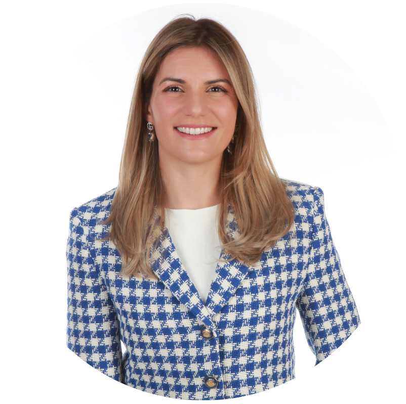
Sharbani Roy, presenter for “What’s New in Machine Learning?”

Sharbani is Sr. Director in Google’s Core Machine Learning group.

Before joining Google, Sharbani led engineering and product teams in Amazon Alexa, focused on media streaming, real-time communication, and applied ML (e.g., NLU, CV, and AR) for 1P/3P developers and end consumers.

Sharbani holds degrees in physics and mathematics from the University of Chicago and an MBA from Stanford University, and lives in Seattle with her husband and three children.


Eve Phillips, presenter for “Future of Frameworks: Navigate the OSS Landscape"

Eve is a Director of Product Management at Google.

Currently, Eve leads the ML Frameworks product team, which includes responsibility for TensorFlow, JAX and Keras. Previously, she led product teams within Google for Clinicians and ChromeOS. Prior to Google, she served as CEO of Empower Interactive, delivering tech-enabled behavioral health.

Earlier, she held roles in leading technology companies and investors including Trilogy, Microsoft, and Greylock.

Eve earned a BS and M.Eng in EECS from MIT and an MBA from Stanford.


Meenu Gaba, presenter for “Data-Centric AI: A New Paradigm"

Meenu leads the Machine Learning infrastructure team at Google, with a mission to power AI innovation with world-class ML infrastructure and services.

She is a technology leader with years of experience launching new products and growing small teams into mature scalable, multi-tiered organizations that are poised to deliver high quality products. Meenu enjoys fast-paced, dynamic, highly iterative/innovative environments and has lots of experience in balancing these disciplines while fostering a people-first culture and forming solid grounds for cross-functional relationships.

Meenu holds a Master's degree in Computer Science. In her free time, she enjoys hiking, solving crosswords, and watching movies.


Kelly Shaefer, presenter for “Maximize Your Data Exploration”

Kelly leads product teams at Google Labs, building both entirely new AI products and AI-enabled features into Google's largest existing products.

In the past, she led the Growth team for Google Workspace, including Gmail, Drive, Docs, and many more.

Outside of Google, she led the Enterprise product team at Stripe and was the P&L owner for Stripe's multi-billion dollar Payments area.

Kelly has an undergraduate degree from Wharton at UPenn, and an MBA from Harvard Business School.


Divyashree Sreepathihalli, presenter for “Keras: Shortcut to AI Mastery”

Divya is a talented machine learning software engineer who is currently a part of the Keras team at Google.

In this role, she specializes in developing Keras core modeling APIs and KerasCV to improve the functionality of the software.

Prior to joining Google, Divya worked as a Deep Learning Scientist for Zazu Sensor, a startup group in Intel's Emerging Growth Incubation (EGI) group. Her work there focused on computer vision and deep learning algorithm development for object detection and tracking, resulting in significant advancements for the startup.

Divya completed her Masters in Computer Engineering from Texas A&M University where she focused on Artificial intelligence in 2017.


Na Li, presenter for “Prototype ML with Visual Blocks”

Na Li is a software engineer manager from Google CoreML.

She leads a team to build developer tools to support ML development journey, from prototyping to model visualization and benchmarking.

Prior to Google, she was a research scientist at Harvard, working in HCI domain.

Throughout her career, Na strives to make ML accessible for everyone.


Zoe Wang, presenter for “Deploying ML Models to Mobile Devices”

Zoe is a technical program manager at Google.

Her career has been focused on Machine Learning (ML) productionization.

Currently she works with her team bringing ML models to mobile devices that power some of AI features for Pixel and other edge devices.

Prior to Google, Zoe worked at Meta on ML Platforms for end-to-end ML lifecycles.


Yvonne Li, presenter for “New GenAI Products and Solutions on Google Cloud”

Yvonne Li is a software engineer on the Duet Platform team at Google, where she focuses on improving the quality of generative AI models.

As a machine learning engineer and developer advocate at IBM, she designed and developed language models and curated open source datasets.

She has over 3 years of experience in the big tech industry, and is passionate about using machine learning to solve real-world problems.

Yvonne is the author of two Coursera courses: Data Analysis with R, and, Data Visualization with R.


Nithya Natesan, presenter for “AI-powered Infrastructure: Cloud TPUs”

Nithya Natesan is a Group Product Manager in the Cloud ML Accelerators team focussing on GPU / TPU offerings for Google Cloud.

Prior to Google, she was head of product management at NVIDIA, launching several products like DGX Cloud, Base Command Platform.

She has ~14 years of experience in hyper convergence Data Center software products, with recent focus on ML / AI Infra and Platform products. She is passionate about building rock solid PM teams, and shipping high quality usable ML / AI products.

Nithya has also won industry accolades namely WomenImpactTech 2023.


Andrada Vulpe, presenter for “Community Matters: 8 Reasons Why You Should Be Involved with Kaggle”

Andrada is a Data Scientist at Endava, a Notebooks Grandmaster on Kaggle, a Dev Expert at Weights and Biases and a proud Z by HP Data Science Global Ambassador.

She is highly passionate about Python, R, Machine and Deep Learning, powerful visualizations and everything in between.

Andrada finished her MSc in Data Science and Analytics in the UK and won 2 Kaggle Analytics competitions.


Jeehae Lee, presenter for “From Recovering Pro Golfer to AI Entrepreneur”

Jeehae Lee is a golf industry executive who has worked to create and build transformational sports technology businesses.

As the Co-Founder & CEO of Sportsbox AI, Jeehae is currently developing products using AI-enabled 3D motion analysis technology that will help participants of various sports and fitness activities learn and improve their skills.

Before founding Sportsbox, she spent five years between 2015 and 2020 at Topgolf Entertainment Group, leading strategy and new business development for various divisions including Toptracer. Between 2012 and 2013, she was at global sports and entertainment marketing agency, IMG, representing professional golfer icon Michelle Wie West. Prior to her career in sports business, she played professional golf at the highest level in the sport, competing on the LPGA tour for three years between 2009 and 2011.

Jeehae is a proud graduate of Phillips Academy in Andover, MA, and has a BA in Economics from Yale and an MBA from The Wharton School at University of Pennsylvania.


Jingwan (Cynthia) Lu, panelist for “The Impact of Generative AI in Different Industries”

Cynthia is a senior director from Adobe leading an applied research organization focusing on developing the Adobe Firefly family of GenAI models built from the ground up.

Her team started training Adobe’s first large-scale foundational model and helped rally together the rest of the company to roll out a new web-based product called Firefly featuring the image generation model as the first step in early 2023.

The same technology and its extension power Adobe Photoshop’s Generative Fill and Generative Expand features giving users intelligent image inpainting and outpainting experience. Time recognizes Adobe Photoshop Generative Fill and Generative Expand as best inventions of 2023 in the AI category.

Before Firefly, Jingwan was a computer vision research scientist and team lead who pioneered and led a large group effort to explore early generative models such as GANs within Adobe.


Wei Xiao, panelist for “The Impact of Generative AI in Different Industries”

Wei is the Director of Developer Relations at NVIDIA for the Middle East, Africa, and emerging regions. Her primary focus is to drive AI and accelerated computing integration within the ecosystem.

Before assuming her current role, Wei Xiao headed Ecosystem Engineering and Evangelism teams at both ARM and Samsung Semiconductor.

In addition to her professional endeavors, Wei dedicates her free time to teaching AI courses at the Graduate School of Computer Science at Santa Clara University.


Priya Mathur, panelist for “The Impact of Generative AI in Different Industries”

Priya is a Staff Data Science Manager at Google and she is the founder of Sparkle – GenAI Data Analyst.

At Google, she leads Data Science for Home Platform Monetization and GenAI efforts for DSPA.

Previously at Groupon, she led Data Science for App Push Notifications and TV Ads.


Katherine Chou, panelist for “The Impact of Generative AI in Different Industries”

Katherine is the Senior Director of Research and Innovations at Google with a specific focus on nurturing scientific and technical breakthroughs that can lead to global impact for science, health, climate, and advancement of platform technologies for our developers and researchers.

Katherine is focused on improving the availability and accuracy of healthcare using machine learning. She is a serial intrapreneur, particularly interested in removing health inequities and improving health and well-being outcomes across all populations.

She previously developed products within Google[x] Labs for Life Sciences (now Verily) and co-founded Medical Brain (now “Health AI'') at Google. She also headed up global teams to develop partner solutions and establish developer ecosystems for Mobile Payments, Mobile Search, GeoCommerce, YouTube, and Android.

Outside of Google, she is a Board member and Program Chair of Lewa Wildlife Conservancy, a Scientific Advisor to the ARCS Foundation, a fellow of the Zoological Society of London, and collaborates with other wildlife NGOs and the Cambridge Business Sustainability Programme in applying the Silicon Valley innovation mindset to new areas.

Katherine holds a double major in Computer Science and Economics at Stanford University and an M.S. in CS specialized in graphics.


Jaimie Hwang, presenter for “Take Action, Learn More, Start Building with Google AI”

Jaimie Hwang is a global product marketing leader with over a decade of experience, specifically in AI/ML.

She has built and led global product marketing teams at a number of AI companies, including an award-winning computer vision startup and tech giant Amazon.

She specializes in executive thought leadership, product storytelling, and integrated GTM strategy. She is passionate about promoting AI technology that is built responsibly and solves real-world problems in a human-centric way.

Jaimie holds a BS in Journalism and Integrated Marketing and Communications from Northwestern University. She lives in Seattle, Washington.


Save your spot at WiML Symposium 2023

The Women in ML Symposium offers sessions for all expertise levels, from beginners to advanced practitioners. RSVP today to secure your spot and explore our comprehensive agenda. We can’t wait to see you there!

Women in ML Symposium 2023: Meet the presenters


Posted by Sharbani Roy – Senior Director, Product Management, Google
We’re back with the third annual Women in Machine Learning Symposium on December 7, 2023

Join us virtually from 9:30 am to 1:00 pm PT for an immersive and insightful set of deep dives for every level of Machine Learning experience.

The Women in ML Symposium is an inclusive event for anyone passionate about the transformative fields of Machine Learning (ML) and Artificial Intelligence (AI). Meet this year’s women in ML as they uncover practical applications across multiple industries and discuss the latest advancements in frameworks, generative AI, and more.


Joana Carrasqueira, presenter for “Enabling Anyone to Build with Google AI”

Joana is a Developer Relations Lead for AI/ML at Google and her mission is to empower individuals and organizations to harness the power of AI to address real-world challenges.

She is a business leader with a track record of bringing strategic vision and global cross-functional programs to life. She’s also the creator of Google’s Women in ML program and flagship symposium, a pioneering initiative that has equipped thousands of developers with knowledge and skills in AI/ML.

Prior to Google, she worked at the Silicon Valley Innovation Center on innovation consulting for Forbes top500, startups and Venture Capital firms. Served as Education Manager at the International Pharmaceutical Federation, working closely with WHO, UNESCO, the United Nations and started her career at the Portuguese Pharmaceutical Society.

Joana holds an MBA from IE Business School, a Master in Pharmaceutical Sciences and a Leadership Certificate from U.C. Berkeley in California.


Sharbani Roy, presenter for “What’s New in Machine Learning?”

Sharbani is Sr. Director in Google’s Core Machine Learning group.

Before joining Google, Sharbani led engineering and product teams in Amazon Alexa, focused on media streaming, real-time communication, and applied ML (e.g., NLU, CV, and AR) for 1P/3P developers and end consumers.

Sharbani holds degrees in physics and mathematics from the University of Chicago and an MBA from Stanford University, and lives in Seattle with her husband and three children.


Eve Phillips, presenter for “Future of Frameworks: Navigate the OSS Landscape"

Eve is a Director of Product Management at Google.

Currently, Eve leads the ML Frameworks product team, which includes responsibility for TensorFlow, JAX and Keras. Previously, she led product teams within Google for Clinicians and ChromeOS. Prior to Google, she served as CEO of Empower Interactive, delivering tech-enabled behavioral health.

Earlier, she held roles in leading technology companies and investors including Trilogy, Microsoft, and Greylock.

Eve earned a BS and M.Eng in EECS from MIT and an MBA from Stanford.


Meenu Gaba, presenter for “Data-Centric AI: A New Paradigm"

Meenu leads the Machine Learning infrastructure team at Google, with a mission to power AI innovation with world-class ML infrastructure and services.

She is a technology leader with years of experience launching new products and growing small teams into mature scalable, multi-tiered organizations that are poised to deliver high quality products. Meenu enjoys fast-paced, dynamic, highly iterative/innovative environments and has lots of experience in balancing these disciplines while fostering a people-first culture and forming solid grounds for cross-functional relationships.

Meenu holds a Master's degree in Computer Science. In her free time, she enjoys hiking, solving crosswords, and watching movies.


Kelly Shaefer, presenter for “Maximize Your Data Exploration”

Kelly leads product teams at Google Labs, building both entirely new AI products and AI-enabled features into Google's largest existing products.

In the past, she led the Growth team for Google Workspace, including Gmail, Drive, Docs, and many more.

Outside of Google, she led the Enterprise product team at Stripe and was the P&L owner for Stripe's multi-billion dollar Payments area.

Kelly has an undergraduate degree from Wharton at UPenn, and an MBA from Harvard Business School.


Divyashree Sreepathihalli, presenter for “Keras: Shortcut to AI Mastery”

Divya is a talented machine learning software engineer who is currently a part of the Keras team at Google.

In this role, she specializes in developing Keras core modeling APIs and KerasCV to improve the functionality of the software.

Prior to joining Google, Divya worked as a Deep Learning Scientist for Zazu Sensor, a startup group in Intel's Emerging Growth Incubation (EGI) group. Her work there focused on computer vision and deep learning algorithm development for object detection and tracking, resulting in significant advancements for the startup.

Divya completed her Masters in Computer Engineering from Texas A&M University where she focused on Artificial intelligence in 2017.


Na Li, presenter for “Prototype ML with Visual Blocks”

Na Li is a software engineer manager from Google CoreML.

She leads a team to build developer tools to support ML development journey, from prototyping to model visualization and benchmarking.

Prior to Google, she was a research scientist at Harvard, working in HCI domain.

Throughout her career, Na strives to make ML accessible for everyone.


Zoe Wang, presenter for “Deploying ML Models to Mobile Devices”

Zoe is a technical program manager at Google.

Her career has been focused on Machine Learning (ML) productionization.

Currently she works with her team bringing ML models to mobile devices that power some of AI features for Pixel and other edge devices.

Prior to Google, Zoe worked at Meta on ML Platforms for end-to-end ML lifecycles.


Yvonne Li, presenter for “New GenAI Products and Solutions on Google Cloud”

Yvonne Li is a software engineer on the Duet Platform team at Google, where she focuses on improving the quality of generative AI models.

As a machine learning engineer and developer advocate at IBM, she designed and developed language models and curated open source datasets.

She has over 3 years of experience in the big tech industry, and is passionate about using machine learning to solve real-world problems.

Yvonne is the author of two Coursera courses: Data Analysis with R, and, Data Visualization with R.


Nithya Natesan, presenter for “AI-powered Infrastructure: Cloud TPUs”

Nithya Natesan is a Group Product Manager in the Cloud ML Accelerators team focussing on GPU / TPU offerings for Google Cloud.

Prior to Google, she was head of product management at NVIDIA, launching several products like DGX Cloud, Base Command Platform.

She has ~14 years of experience in hyper convergence Data Center software products, with recent focus on ML / AI Infra and Platform products. She is passionate about building rock solid PM teams, and shipping high quality usable ML / AI products.

Nithya has also won industry accolades namely WomenImpactTech 2023.


Andrada Vulpe, presenter for “Community Matters: 8 Reasons Why You Should Be Involved with Kaggle”

Andrada is a Data Scientist at Endava, a Notebooks Grandmaster on Kaggle, a Dev Expert at Weights and Biases and a proud Z by HP Data Science Global Ambassador.

She is highly passionate about Python, R, Machine and Deep Learning, powerful visualizations and everything in between.

Andrada finished her MSc in Data Science and Analytics in the UK and won 2 Kaggle Analytics competitions.


Jeehae Lee, presenter for “From Recovering Pro Golfer to AI Entrepreneur”

Jeehae Lee is a golf industry executive who has worked to create and build transformational sports technology businesses.

As the Co-Founder & CEO of Sportsbox AI, Jeehae is currently developing products using AI-enabled 3D motion analysis technology that will help participants of various sports and fitness activities learn and improve their skills.

Before founding Sportsbox, she spent five years between 2015 and 2020 at Topgolf Entertainment Group, leading strategy and new business development for various divisions including Toptracer. Between 2012 and 2013, she was at global sports and entertainment marketing agency, IMG, representing professional golfer icon Michelle Wie West. Prior to her career in sports business, she played professional golf at the highest level in the sport, competing on the LPGA tour for three years between 2009 and 2011.

Jeehae is a proud graduate of Phillips Academy in Andover, MA, and has a BA in Economics from Yale and an MBA from The Wharton School at University of Pennsylvania.


Jingwan (Cynthia) Lu, panelist for “The Impact of Generative AI in Different Industries”

Cynthia is a senior director from Adobe leading an applied research organization focusing on developing the Adobe Firefly family of GenAI models built from the ground up.

Her team started training Adobe’s first large-scale foundational model and helped rally together the rest of the company to roll out a new web-based product called Firefly featuring the image generation model as the first step in early 2023.

The same technology and its extension power Adobe Photoshop’s Generative Fill and Generative Expand features giving users intelligent image inpainting and outpainting experience. Time recognizes Adobe Photoshop Generative Fill and Generative Expand as best inventions of 2023 in the AI category.

Before Firefly, Jingwan was a computer vision research scientist and team lead who pioneered and led a large group effort to explore early generative models such as GANs within Adobe.


Wei Xiao, panelist for “The Impact of Generative AI in Different Industries”

Wei is the Director of Developer Relations at NVIDIA for the Middle East, Africa, and emerging regions. Her primary focus is to drive AI and accelerated computing integration within the ecosystem.

Before assuming her current role, Wei Xiao headed Ecosystem Engineering and Evangelism teams at both ARM and Samsung Semiconductor.

In addition to her professional endeavors, Wei dedicates her free time to teaching AI courses at the Graduate School of Computer Science at Santa Clara University.


Priya Mathur, panelist for “The Impact of Generative AI in Different Industries”

Priya is a Staff Data Science Manager at Google and she is the founder of Sparkle – GenAI Data Analyst.

At Google, she leads Data Science for Home Platform Monetization and GenAI efforts for DSPA.

Previously at Groupon, she led Data Science for App Push Notifications and TV Ads.


Katherine Chou, panelist for “The Impact of Generative AI in Different Industries”

Katherine is the Senior Director of Research and Innovations at Google with a specific focus on nurturing scientific and technical breakthroughs that can lead to global impact for science, health, climate, and advancement of platform technologies for our developers and researchers.

Katherine is focused on improving the availability and accuracy of healthcare using machine learning. She is a serial intrapreneur, particularly interested in removing health inequities and improving health and well-being outcomes across all populations.

She previously developed products within Google[x] Labs for Life Sciences (now Verily) and co-founded Medical Brain (now “Health AI'') at Google. She also headed up global teams to develop partner solutions and establish developer ecosystems for Mobile Payments, Mobile Search, GeoCommerce, YouTube, and Android.

Outside of Google, she is a Board member and Program Chair of Lewa Wildlife Conservancy, a Scientific Advisor to the ARCS Foundation, a fellow of the Zoological Society of London, and collaborates with other wildlife NGOs and the Cambridge Business Sustainability Programme in applying the Silicon Valley innovation mindset to new areas.

Katherine holds a double major in Computer Science and Economics at Stanford University and an M.S. in CS specialized in graphics.


Jaimie Hwang, presenter for “Take Action, Learn More, Start Building with Google AI”

Jaimie Hwang is a global product marketing leader with over a decade of experience, specifically in AI/ML.

She has built and led global product marketing teams at a number of AI companies, including an award-winning computer vision startup and tech giant Amazon.

She specializes in executive thought leadership, product storytelling, and integrated GTM strategy. She is passionate about promoting AI technology that is built responsibly and solves real-world problems in a human-centric way.

Jaimie holds a BS in Journalism and Integrated Marketing and Communications from Northwestern University. She lives in Seattle, Washington.


Save your spot at WiML Symposium 2023

The Women in ML Symposium offers sessions for all expertise levels, from beginners to advanced practitioners. RSVP today to secure your spot and explore our comprehensive agenda. We can’t wait to see you there!

Alternating updates for efficient transformers

Contemporary deep learning models have been remarkably successful in many domains, ranging from natural language to computer vision. Transformer neural networks (transformers) are a popular deep learning architecture that today comprise the foundation for most tasks in natural language processing and also are starting to extend to applications in other domains, such as computer vision, robotics, and autonomous driving. Moreover, they form the backbone of all the current state-of-the-art language models.

Increasing scale in Transformer networks has led to improved performance and the emergence of behavior not present in smaller networks. However, this increase in scale often comes with prohibitive increases in compute cost and inference latency. A natural question is whether we can reap the benefits of larger models without incurring the computational burden.

In “Alternating Updates for Efficient Transformers”, accepted as a Spotlight at NeurIPS 2023, we introduce AltUp, a method to take advantage of increased token representation without increasing the computation cost. AltUp is easy to implement, widely applicable to any transformer architecture, and requires minimal hyperparameter tuning. For instance, using a variant of AltUp on a 770M parameter T5-Large model, the addition of ~100 parameters yields a model with a significantly better quality.


Background

To understand how we can achieve this, we dig into how transformers work. First, they partition the input into a sequence of tokens. Each token is then mapped to an embedding vector (via the means of an embedding table) called the token embedding. We call the dimension of this vector the token representation dimension. The Transformer then operates on this sequence of token embeddings by applying a series of computation modules (called layers) using its network parameters. The number of parameters in each transformer layer is a function of the layer’s width, which is determined by the token representation dimension.

To achieve benefits of scale without incurring the compute burden, prior works such as sparse mixture-of-experts (Sparse MoE) models (e.g., Switch Transformer, Expert Choice, V-MoE) have predominantly focused on efficiently scaling up the network parameters (in the self-attention and feedforward layers) by conditionally activating a subset based on the input. This allows us to scale up network size without significantly increasing compute per input. However, there is a research gap on scaling up the token representation dimension itself by conditionally activating parts of the token representation vector.

Recent works (for example, scaling laws and infinite-width networks) have empirically and theoretically established that a wider token representation helps in learning more complicated functions. This phenomenon is also evident in modern architectures of increasing capability. For instance, the representation dimension grows from 512 (small) to 768 (base) and 1024 (corresponding to models with 770M, 3B, and 11B parameters respectively) in T5 models, and from 4096 (8B) to 8192 (64B) and 18432 (540B) in PaLM models. A widened representation dimension also significantly improves performance for dual encoder retrieval models. However, naïvely widening the representation vector requires one to increase the model dimension accordingly, which quadratically1 increases the amount of computation in the feedforward computation.


Method

AltUp works by partitioning a widened representation vector into equal sized blocks, processing only a single block at each layer, and using an efficient prediction-correction mechanism to infer the outputs of the other blocks (shown below on the right). This allows AltUp to simultaneously keep the model dimension, hence the computation cost, roughly constant and take advantage of using an increased token dimension. The increased token dimension allows the model to pack more information into each token’s embedding. By keeping the width of each transformer layer constant, AltUp avoids incurring the quadratic increase in computation cost that would otherwise be present with a naïve expansion of the representation.

An illustration of widening the token representation without (left) and with AltUp (right). This widening causes a near-quadratic increase in computation in a vanilla transformer due to the increased layer width. In contrast, Alternating Updates keeps the layer width constant and efficiently computes the output by operating on a sub-block of the representation at each layer.

More specifically, the input to each layer is two or more blocks, one of which is passed into the 1x width transformer layer (see figure below). We refer to this block as the “activated” block. This computation results in the exact output for the activated block. In parallel, we invoke a lightweight predictor that computes a weighted combination of all the input blocks. The predicted values, along with the computed value of the activated block, are passed on to a lightweight corrector that updates the predictions based on the observed values. This correction mechanism enables the inactivated blocks to be updated as a function of the activated one. Both the prediction and correction steps only involve a limited number of vector additions and multiplications and hence are much faster than a regular transformer layer. We note that this procedure can be generalized to an arbitrary number of blocks.

The predictor and corrector computations: The predictor mixes sub-blocks with trainable scalar coefficients; the corrector returns a weighted average of the predictor output and the transformer output. The predictor and corrector perform scalar-vector multiplications and incur negligible computation cost compared to the transformer. The predictor outputs a linear mixing of blocks with scalar mixing coefficients pi, j , and the corrector combines predictor output and transformer output with weights gi.

At a higher level, AltUp is similar to sparse MoE in that it is a method to add capacity to a model in the form of conditionally accessed (external) parameters. In sparse MoE, the additional parameters take the form of feed forward network (FFN) experts and the conditionality is with respect to the input. In AltUp, the external parameters come from the widened embedding table and the conditionality takes the form of alternating block-wise activation of the representation vector, as in the figure above. Hence, AltUp has the same underpinning as sparse MoE models.

An advantage of AltUp over sparse MoE is that it does not necessitate sharding since the number of additional parameters introduced is a factor2 of the embedding table size, which typically makes up a small fraction of the overall model size. Moreover, since AltUp focuses on conditionally activating parts of a wider token representation, it can be applied synergistically with orthogonal techniques like MoE to obtain complementary performance gains.


Evaluation

AltUp was evaluated on T5 models on various benchmark language tasks. Models augmented with AltUp are uniformly faster than the extrapolated dense models at the same accuracy. For example, we observe that a T5 Large model augmented with AltUp leads to a 27%, 39%, 87%, and 29% speedup on GLUE, SuperGLUE, SQuAD, and Trivia-QA benchmarks, respectively.

Evaluations of AltUp on T5 models of various sizes and popular benchmarks. AltUp consistently leads to sizable speedups relative to baselines at the same accuracy. Latency is measured on TPUv3 with 8 cores. Speedup is defined as the change in latency divided by the AltUp latency (B = T5 Base, L = T5 Large, XL = T5 XL models).

AltUp’s relative performance improves as we apply it to larger models — compare the relative speedup of T5 Base + AltUp to that of T5 Large + AltUp. This demonstrates the scalability of AltUp and its improved performance on even larger models. Overall, AltUp consistently leads to models with better predictive performance than the corresponding baseline models with the same speed on all evaluated model sizes and benchmarks.


Extensions: Recycled AltUp

The AltUp formulation adds an insignificant amount of per-layer computation, however, it does require using a wider embedding table. In certain scenarios where the vocabulary size (i.e., the number of distinct tokens the tokenizer can produce) is very large, this may lead to a non-trivial amount of added computation for the initial embedding lookup and the final linear + softmax operation. A very large vocabulary may also lead to an undesirable amount of added embedding parameters. To address this, Recycled-AltUp is an extension of AltUp that avoids these computational and parameter costs by keeping the embedding table's width the same.

Illustration of the Architecture for Recycled-AltUp with K = 2.

In Recycled-AltUp, instead of widening the initial token embeddings, we replicate the embeddings K times to form a wider token representation. Hence, Recycled-AltUp adds virtually no additional parameters relative to the baseline transformer, while benefiting from a wider token representation.

Recycled-AltUp on T5-B/L/XL compared to baselines. Recycled-AltUp leads to strict improvements in pre-training performance without incurring any perceptible slowdown.

We also evaluate the lightweight extension of AltUp, Recycled-AltUp, with K = 2 on T5 base, large, and XL models and compare its pre-trained accuracy and speed to those of baselines. Since Recycled-AltUp does not require an expansion in the embedding table dimension, the models augmented with it have virtually the same number of trainable parameters as the baseline models. We again observe consistent improvements compared to the dense baselines.


Why does AltUp work?

AltUp increases a model’s capacity by adding and efficiently leveraging auxiliary parameters to the embedding table, and maintaining the higher dimensional representation across the layers. We believe that a key ingredient in this computation lies in AltUp’s prediction mechanism that performs an ensemble of the different blocks. This weighted combination enables continuous message passing to the entire vector despite activating only sub-blocks of it in each layer. Recycled-AltUp, on the other hand, does not add any additional parameters to the token embeddings. However, it still confers the benefit of simulating computation in a higher dimensional representation space since a higher dimensional representation vector is maintained when moving from one transformer layer to another. We conjecture that this aids the training by augmenting the flow of information through the network. An interesting research direction is to explore whether the benefits of Recycled-AltUp can be explained entirely by more favorable training dynamics.


Acknowledgements

We thank our collaborators Cenk Baykal, Dylan Cutler, and Rina Panigrahy at Google Research, and Nikhil Ghosh at University of California, Berkeley (work done during research internship at Google).


1This is because the feedforward layers of a Transformer are typically scaled quadratically with the model dimension. 
2This factor depends on the user-specified expansion factor, but is typically 1, i.e., we double the embedding table dimension. 

Source: Google AI Blog


Zero-shot adaptive prompting of large language models

Recent advances in large language models (LLMs) are very promising as reflected in their capability for general problem-solving in few-shot and zero-shot setups, even without explicit training on these tasks. This is impressive because in the few-shot setup, LLMs are presented with only a few question-answer demonstrations prior to being given a test question. Even more challenging is the zero-shot setup, where the LLM is directly prompted with the test question only.

Even though the few-shot setup has dramatically reduced the amount of data required to adapt a model for a specific use-case, there are still cases where generating sample prompts can be challenging. For example, handcrafting even a small number of demos for the broad range of tasks covered by general-purpose models can be difficult or, for unseen tasks, impossible. For example, for tasks like summarization of long articles or those that require domain knowledge (e.g., medical question answering), it can be challenging to generate sample answers. In such situations, models with high zero-shot performance are useful since no manual prompt generation is required. However, zero-shot performance is typically weaker as the LLM is not presented with guidance and thus is prone to spurious output.

In “Better Zero-shot Reasoning with Self-Adaptive Prompting”, published at ACL 2023, we propose Consistency-Based Self-Adaptive Prompting (COSP) to address this dilemma. COSP is a zero-shot automatic prompting method for reasoning problems that carefully selects and constructs pseudo-demonstrations for LLMs using only unlabeled samples (that are typically easy to obtain) and the models’ own predictions. With COSP, we largely close the performance gap between zero-shot and few-shot while retaining the desirable generality of zero-shot prompting. We follow this with “Universal Self-Adaptive Prompting“ (USP), accepted at EMNLP 2023, in which we extend the idea to a wide range of general natural language understanding (NLU) and natural language generation (NLG) tasks and demonstrate its effectiveness.


Prompting LLMs with their own outputs

Knowing that LLMs benefit from demonstrations and have at least some zero-shot abilities, we wondered whether the model’s zero-shot outputs could serve as demonstrations for the model to prompt itself. The challenge is that zero-shot solutions are imperfect, and we risk giving LLMs poor quality demonstrations, which could be worse than no demonstrations at all. Indeed, the figure below shows that adding a correct demonstration to a question can lead to a correct solution of the test question (Demo1 with question), whereas adding an incorrect demonstration (Demo 2 + questions, Demo 3 with questions) leads to incorrect answers. Therefore, we need to select reliable self-generated demonstrations.

Example inputs & outputs for reasoning tasks, which illustrates the need for carefully designed selection procedure for in-context demonstrations (MultiArith dataset & PaLM-62B model): (1) zero-shot chain-of-thought with no demo: correct logic but wrong answer; (2) correct demo (Demo1) and correct answer; (3) correct but repetitive demo (Demo2) leads to repetitive outputs; (4) erroneous demo (Demo3) leads to a wrong answer; but (5) combining Demo3 and Demo1 again leads to a correct answer.

COSP leverages a key observation of LLMs: that confident and consistent predictions are more likely correct. This observation, of course, depends on how good the uncertainty estimate of the LLM is. Luckily, in large models, previous works suggest that the uncertainty estimates are robust. Since measuring confidence requires only model predictions, not labels, we propose to use this as a zero-shot proxy of correctness. The high-confidence outputs and their inputs are then used as pseudo-demonstrations.

With this as our starting premise, we estimate the model’s confidence in its output based on its self-consistency and use this measure to select robust self-generated demonstrations. We ask LLMs the same question multiple times with zero-shot chain-of-thought (CoT) prompting. To guide the model to generate a range of possible rationales and final answers, we include randomness controlled by a “temperature” hyperparameter. In an extreme case, if the model is 100% certain, it should output identical final answers each time. We then compute the entropy of the answers to gauge the uncertainty — the answers that have high self-consistency and for which the LLM is more certain, are likely to be correct and will be selected.

Assuming that we are presented with a collection of unlabeled questions, the COSP method is:

  1. Input each unlabeled question into an LLM, obtaining multiple rationales and answers by sampling the model multiple times. The most frequent answers are highlighted, followed by a score that measures consistency of answers across multiple sampled outputs (higher is better). In addition to favoring more consistent answers, we also penalize repetition within a response (i.e., with repeated words or phrases) and encourage diversity of selected demonstrations. We encode the preference towards consistent, un-repetitive and diverse outputs in the form of a scoring function that consists of a weighted sum of the three scores for selection of the self-generated pseudo-demonstrations.
  2. We concatenate the pseudo-demonstrations into test questions, feed them to the LLM, and obtain a final predicted answer.
Illustration of COSP: In Stage 1 (left), we run zero-shot CoT multiple times to generate a pool of demonstrations (each consisting of the question, generated rationale and prediction) and assign a score. In Stage 2 (right), we augment the current test question with pseudo-demos (blue boxes) and query the LLM again. A majority vote over outputs from both stages forms the final prediction.

COSP focuses on question-answering tasks with CoT prompting for which it is easy to measure self-consistency since the questions have unique correct answers. But this can be difficult for other tasks, such as open-ended question-answering or generative tasks that don’t have unique answers (e.g., text summarization). To address this limitation, we introduce USP in which we generalize our approach to other general NLP tasks:

  • Classification (CLS): Problems where we can compute the probability of each class using the neural network output logits of each class. In this way, we can measure the uncertainty without multiple sampling by computing the entropy of the logit distribution.
  • Short-form generation (SFG): Problems like question answering where we can use the same procedure mentioned above for COSP, but, if necessary, without the rationale-generating step.
  • Long-form generation (LFG): Problems like summarization and translation, where the questions are often open-ended and the outputs are unlikely to be identical, even if the LLM is certain. In this case, we use an overlap metric in which we compute the average of the pairwise ROUGE score between the different outputs to the same query.
Illustration of USP in exemplary tasks (classification, QA and text summarization). Similar to COSP, the LLM first generates predictions on an unlabeled dataset whose outputs are scored with logit entropy, consistency or alignment, depending on the task type, and pseudo-demonstrations are selected from these input-output pairs. In Stage 2, the test instances are augmented with pseudo-demos for prediction.

We compute the relevant confidence scores depending on the type of task on the aforementioned set of unlabeled test samples. After scoring, similar to COSP, we pick the confident, diverse and less repetitive answers to form a model-generated pseudo-demonstration set. We finally query the LLM again in a few-shot format with these pseudo-demonstrations to obtain the final predictions on the entire test set.


Key Results

For COSP, we focus on a set of six arithmetic and commonsense reasoning problems, and we compare against 0-shot-CoT (i.e., “Let’s think step by step“ only). We use self-consistency in all baselines so that they use roughly the same amount of computational resources as COSP. Compared across three LLMs, we see that zero-shot COSP significantly outperforms the standard zero-shot baseline.

Key results of COSP in six arithmetic (MultiArith, GSM-8K, AddSub, SingleEq) and commonsense (CommonsenseQA, StrategyQA) reasoning tasks using PaLM-62B, PaLM-540B and GPT-3 (code-davinci-001) models.

USP improves significantly on 0-shot performance. “CLS” is an average of 15 classification tasks; “SFG” is the average of five short-form generation tasks; “LFG” is the average of two summarization tasks. “SFG (BBH)” is an average of all BIG-Bench Hard tasks, where each question is in SFG format.

For USP, we expand our analysis to a much wider range of tasks, including more than 25 classifications, short-form generation, and long-form generation tasks. Using the state-of-the-art PaLM 2 models, we also test against the BIG-Bench Hard suite of tasks where LLMs have previously underperformed compared to people. We show that in all cases, USP again outperforms the baselines and is competitive to prompting with golden examples.

Accuracy on BIG-Bench Hard tasks with PaLM 2-M (each line represents a task of the suite). The gain/loss of USP (green stars) over standard 0-shot (green triangles) is shown in percentages. “Human” refers to average human performance; “AutoCoT” and “Random demo” are baselines we compared against in the paper; and “3-shot” is the few-shot performance for three handcrafted demos in CoT format.

We also analyze the working mechanism of USP by validating the key observation above on the relation between confidence and correctness, and we found that in an overwhelming majority of the cases, USP picks confident predictions that are more likely better in all task types considered, as shown in the figure below.

USP picks confident predictions that are more likely better. Ground-truth performance metrics against USP confidence scores in selected tasks in various task types (blue: CLS, orange: SFG, green: LFG) with PaLM-540B.

Conclusion

Zero-shot inference is a highly sought-after capability of modern LLMs, yet the success in which poses unique challenges. We propose COSP and USP, a family of versatile, zero-shot automatic prompting techniques applicable to a wide range of tasks. We show large improvement over the state-of-the-art baselines over numerous task and model combinations.


Acknowledgements

This work was conducted by Xingchen Wan, Ruoxi Sun, Hootan Nakhost, Hanjun Dai, Julian Martin Eisenschlos, Sercan Ö. Arık, and Tomas Pfister. We would like to thank Jinsung Yoon Xuezhi Wang for providing helpful reviews, and other colleagues at Google Cloud AI Research for their discussion and feedback.

Source: Google AI Blog


MetNet-3: A state-of-the-art neural weather model available in Google products

Forecasting weather variables such as precipitation, temperature, and wind is key to numerous aspects of society, from daily planning and transportation to energy production. As we continue to see more extreme weather events such as floods, droughts, and heat waves, accurate forecasts can be essential to preparing for and mitigating their effects. The first 24 hours into the future are especially important as they are both highly predictable and actionable, which can help people make informed decisions in a timely manner and stay safe.

Today we present a new weather model called MetNet-3, developed by Google Research and Google DeepMind. Building on the earlier MetNet and MetNet-2 models, MetNet-3 provides high resolution predictions up to 24 hours ahead for a larger set of core variables, including precipitation, surface temperature, wind speed and direction, and dew point. MetNet-3 creates a temporally smooth and highly granular forecast, with lead time intervals of 2 minutes and spatial resolutions of 1 to 4 kilometers. MetNet-3 achieves strong performance compared to traditional methods, outperforming the best single- and multi-member physics-based numerical weather prediction (NWP) models — such as High-Resolution Rapid Refresh (HRRR) and ensemble forecast suite (ENS) — for multiple regions up to 24 hours ahead.

Finally, we’ve integrated MetNet-3’s capabilities across various Google products and technologies where weather is relevant. Currently available in the contiguous United States and parts of Europe with a focus on 12 hour precipitation forecasts, MetNet-3 is helping bring accurate and reliable weather information to people in multiple countries and languages.

     
MetNet-3 precipitation output summarized into actionable forecasts in Google Search on mobile.

Densification of sparse observations

Many recent machine learning weather models use the atmospheric state generated by traditional methods (e.g., data assimilation from NWPs) as the primary starting point to build forecasts. In contrast, a defining feature of the MetNet models has been to use direct observations of the atmosphere for training and evaluation. The advantage of direct observations is that they often have higher fidelity and resolution. However, direct observations come from a large variety of sensors at different altitudes, including weather stations at the surface level and satellites in orbit, and can be of varying degrees of sparsity. For example, precipitation estimates derived from radar such as NOAA’s Multi-Radar/Multi-Sensor System (MRMS) are relatively dense images, whereas weather stations located on the ground that provide measurements for variables such as temperature and wind are mere points spread over a region.

In addition to the data sources used in previous MetNet models, MetNet-3 includes point measurements from weather stations as both inputs and targets with the goal of making a forecast at all locations. To this end, MetNet-3’s key innovation is a technique called densification, which merges the traditional two-step process of data assimilation and simulation found in physics-based models into a single pass through the neural network. The main components of densification are illustrated below. Although the densification technique applies to a specific stream of data individually, the resulting densified forecast benefits from all the other input streams that go into MetNet-3, including topographical, satellite, radar, and NWP analysis features. No NWP forecasts are included in MetNet-3’s default inputs.

A) During training, a fraction of the weather stations are masked out from the input while kept in the target. B) To evaluate generalization to untrained locations, a set of weather stations represented by squares is never used for training and is only used for evaluation. C) Data from these held out weather stations with sparse coverage is included during evaluation to determine prediction quality in these areas. D) The final forecasts use the full set of training weather stations as input and produce fully dense forecasts aided by spatial parameter sharing.

High resolution in space and time

A central advantage of using direct observations is their high spatial and temporal resolution. For example, weather stations and ground radar stations provide measurements every few minutes at specific points and at 1 km resolutions, respectively; this is in stark contrast with the assimilation state from the state-of-the-art model ENS, which is generated every 6 hours at a resolution of 9 km with hour-by-hour forecasts. To handle such a high resolution, MetNet-3 preserves another of the defining features of this series of models, lead time conditioning. The lead time of the forecast in minutes is directly given as input to the neural network. This allows MetNet-3 to efficiently model the high temporal frequency of the observations for intervals as brief as 2 minutes. Densification combined with lead time conditioning and high resolution direct observations produces a fully dense 24 hour forecast with a temporal resolution of 2 minutes, while learning from just 1,000 points from the One Minute Observation (OMO) network of weather stations spread across the United States.

MetNet-3 predicts a marginal multinomial probability distribution for each output variable and each location that provides rich information beyond just the mean. This allows us to compare the probabilistic outputs of MetNet-3 with the outputs of advanced probabilistic ensemble NWP models, including the ensemble forecast ENS from the European Centre for Medium-Range Weather Forecasts and the High Resolution Ensemble Forecast (HREF) from the National Oceanic and Atmospheric Administration of the US. Due to the probabilistic nature of the outputs of both models, we are able to compute scores such as the Continuous Ranked Probability Score (CRPS). The following graphics highlight densification results and illustrate that MetNet’s forecasts are not only of much higher resolution, but are also more accurate when evaluated at the overlapping lead times.

Top: MetNet-3’s forecast of wind speed for each 2 minutes over the future 24 hours with a spatial resolution of 4km. Bottom: ENS’s hourly forecast with a spatial resolution of 18 km.
The two distinct regimes in spatial structure are primarily driven by the presence of the Colorado mountain ranges. Darker corresponds to higher wind speed. More samples available here: 1, 2, 3, 4.
Performance comparison between MetNet-3 and NWP baseline for wind speed based on CRPS (lower is better). In the hyperlocal setting, values of the test weather stations are given as input to the network during evaluation; the results improve further especially in the early lead times.

In contrast to weather station variables, precipitation estimates are more dense as they come from ground radar. MetNet-3’s modeling of precipitation is similar to that of MetNet-1 and 2, but extends the high resolution precipitation forecasts with a 1km spatial granularity to the same 24 hours of lead time as the other variables, as shown in the animation below. MetNet-3’s performance on precipitation achieves a better CRPS value than ENS’s throughout the 24 hour range.

Case study for Thu Jan 17 2019 00:00 UTC showing the probability of instantaneous precipitation rate being above 1 mm/h on CONUS. Darker corresponds to a higher probability value. The maps also show the prediction threshold when optimized towards Critical Success Index CSI (dark blue contours). This specific case study shows the formation of a new large precipitation pattern in the central US; it is not just forecasting of existing patterns.
Top: ENS’s hourly forecast. Center: Ground truth, source NOAA’s MRMS. Bottom: Probability map as predicted by MetNet-3. Native resolution available here.
Performance comparison between MetNet-3 and NWP baseline for instantaneous precipitation rate on CRPS (lower is better).

Delivering realtime ML forecasts

Training and evaluating a weather forecasting model like MetNet-3 on historical data is only a part of the process of delivering ML-powered forecasts to users. There are many considerations when developing a real-time ML system for weather forecasting, such as ingesting real-time input data from multiple distinct sources, running inference, implementing real-time validation of outputs, building insights from the rich output of the model that lead to an intuitive user experience, and serving the results at Google scale — all on a continuous cycle, refreshed every few minutes.

We developed such a real-time system that is capable of producing a precipitation forecast every few minutes for the entire contiguous United States and for 27 countries in Europe for a lead time of up to 12 hours.

Illustration of the process of generating precipitation forecasts using MetNet-3.

The system's uniqueness stems from its use of near-continuous inference, which allows the model to constantly create full forecasts based on incoming data streams. This mode of inference is different from traditional inference systems, and is necessary due to the distinct characteristics of the incoming data. The model takes in various data sources as input, such as radar, satellite, and numerical weather prediction assimilations. Each of these inputs has a different refresh frequency and spatial and temporal resolution. Some data sources, such as weather observations and radar, have characteristics similar to a continuous stream of data, while others, such as NWP assimilations, are similar to batches of data. The system is able to align all of these data sources spatially and temporally, allowing the model to create an updated understanding of the next 12 hours of precipitation at a very high cadence.

With the above process, the model is able to predict arbitrary discrete probability distributions. We developed novel techniques to transform this dense output space into user-friendly information that enables rich experiences throughout Google products and technologies.


Weather features in Google products

People around the world rely on Google every day to provide helpful, timely, and accurate information about the weather. This information is used for a variety of purposes, such as planning outdoor activities, packing for trips, and staying safe during severe weather events.

The state-of-the-art accuracy, high temporal and spatial resolution, and probabilistic nature of MetNet-3 makes it possible to create unique hyperlocal weather insights. For the contiguous United States and Europe, MetNet-3 is operational and produces real-time 12 hour precipitation forecasts that are now served across Google products and technologies where weather is relevant, such as Search. The rich output from the model is synthesized into actionable information and instantly served to millions of users.

For example, a user who searches for weather information for a precise location from their mobile device will receive highly localized precipitation forecast data, including timeline graphs with granular minute breakdowns depending on the product.

MetNet-3 precipitation output in weather on the Google app on Android (left) and mobile web Search (right).

Conclusion

MetNet-3 is a new deep learning model for weather forecasting that outperforms state-of-the-art physics-based models for 24-hour forecasts of a core set of weather variables. It has the potential to create new possibilities for weather forecasting and to improve the safety and efficiency of many activities, such as transportation, agriculture, and energy production. MetNet-3 is operational and its forecasts are served across several Google products where weather is relevant.


Acknowledgements

Many people were involved in the development of this effort. We would like to especially thank those from Google DeepMind (Di Li, Jeremiah Harmsen, Lasse Espeholt, Marcin Andrychowicz, Zack Ontiveros), Google Research (Aaron Bell, Akib Uddin, Alex Merose, Carla Bromberg, Fred Zyda, Isalo Montacute, Jared Sisk, Jason Hickey, Luke Barrington, Mark Young, Maya Tohidi, Natalie Williams, Pramod Gupta, Shreya Agrawal, Thomas Turnbull, Tom Small, Tyler Russell), and Google Search (Agustin Pesciallo, Bill Myers, Danny Cheresnick, Lior Cohen, Maca Piombi, Maia Diamant, Max Kamenetsky, Maya Ekron, Mor Schlesinger, Neta Gefen-Doron, Nofar Peled Levi, Ofer Lehr, Or Hillel, Rotem Wertman, Vinay Ruelius Shah, Yechie Labai).

Source: Google AI Blog


Looking back at wildfire research in 2023

Wildfires are becoming larger and affecting more and more communities around the world, often resulting in large-scale devastation. Just this year, communities have experienced catastrophic wildfires in Greece, Maui, and Canada to name a few. While the underlying causes leading to such an increase are complex — including changing climate patterns, forest management practices, land use development policies and many more — it is clear that the advancement of technologies can help to address the new challenges.

At Google Research, we’ve been investing in a number of climate adaptation efforts, including the application of machine learning (ML) to aid in wildfire prevention and provide information to people during these events. For example, to help map fire boundaries, our wildfire boundary tracker uses ML models and satellite imagery to map large fires in near real-time with updates every 15 minutes. To advance our various research efforts, we are partnering with wildfire experts and government agencies around the world.

Today we are excited to share more about our ongoing collaboration with the US Forest Service (USFS) to advance fire modeling tools and fire spread prediction algorithms. Starting from the newly developed USFS wildfire behavior model, we use ML to significantly reduce computation times, thus enabling the model to be employed in near real time. This new model is also capable of incorporating localized fuel characteristics, such as fuel type and distribution, in its predictions. Finally, we describe an early version of our new high-fidelity 3D fire spread model.


Current state of the art in wildfire modeling

Today’s most widely used state-of-the-art fire behavior models for fire operation and training are based on the Rothermel fire model developed at the US Forest Service Fire Lab, by Rothermel et al., in the 1970s. This model considers many key factors that affect fire spread, such as the influence of wind, the slope of the terrain, the moisture level, the fuel load (e.g., the density of the combustible materials in the forest), etc., and provided a good balance between computational feasibility and accuracy at the time. The Rothermel model has gained widespread use throughout the fire management community across the world.

Various operational tools that employ the Rothermel model, such as BEHAVE, FARSITE, FSPro, and FlamMap, have been developed and improved over the years. These tools and the underlying model are used mainly in three important ways: (1) for training firefighters and fire managers to develop their insights and intuitions on fire behavior, (2) for fire behavior analysts to predict the development of a fire during a fire operation and to generate guidance for situation awareness and resource allocation planning, and (3) for analyzing forest management options intended to mitigate fire hazards across large landscapes.  These models are the foundation of fire operation safety and efficiency today.

However, there are limitations on these state-of-the art models, mostly associated with the simplification of the underlying physical processes (which was necessary when these models were created). By simplifying the physics to produce steady state predictions, the required inputs for fuel sources and weather became practical but also more abstract compared to measurable quantities.  As a result, these models are typically “adjusted” and “tweaked” by experienced fire behavior analysts so they work more accurately in certain situations and to compensate for uncertainties and unknowable environmental characteristics. Yet these expert adjustments mean that many of the calculations are not repeatable.

To overcome these limitations, USFS researchers have been working on a new model to drastically improve the physical fidelity of fire behavior prediction. This effort represents the first major shift in fire modeling in the past 50 years. While the new model continues to improve in capturing fire behavior, the computational cost and inference time makes it impractical to be deployed in the field or for applications with near real-time requirements. In a realistic scenario, to make this model useful and practical in training and operations, a speed up of at least 1000x would be needed.


Machine learning acceleration

In partnership with the USFS, we have undertaken a program to apply ML to decrease computation times for complex fire models. Researchers knew that many complex inputs and features could be characterized using a deep neural network, and if successful, the trained model would lower the computational cost and latency of evaluating new scenarios. Deep learning is a branch of machine learning that uses neural networks with multiple hidden layers of nodes that do not directly correspond to actual observations. The model’s hidden layers allow a rich representation of extremely complex systems — an ideal technique for modeling wildfire spread.

We used the USFS physics-based, numerical prediction models to generate many simulations of wildfire behavior and then used these simulated examples to train the deep learning model on the inputs and features to best capture the system behavior accurately. We found that the deep learning model can perform at a much lower computational cost compared to the original and is able to address behaviors resulting from fine-scale processes. In some cases, computation time for capturing the fine-scale features described above and providing a fire spread estimate was 100,000 times faster than running the physics-based numerical models.

This project has continued to make great progress since the first report at presentation at ICFFR 2022 and the USFS Fire Lab's project page provides a glimpse into the ongoing work in this direction. Our team has expanded the dataset used for training by an order of magnitude, from 40M up to 550M training examples. Additionally, we have delivered a prototype ML model that our USFS Fire Lab partner is integrating into a training app that is currently being developed for release in 2024.

Google researchers visiting the USFS Fire Lab in Missoula, MT, stopping by Big Knife Fire Operation Command Center.

Fine-grained fuel representation

Besides training, another key use-case of the new model is for operational fire prediction. To fully leverage the advantages of the new model’s capability to capture the detailed fire behavior changes from small-scale differences in fuel structures, high resolution fuel mapping and representation are needed. To this end, we are currently working on the integration of high resolution satellite imagery and geo information into ML models to allow fuel specific mapping at-scale. Some of the preliminary results will be presented at the upcoming 10th International Fire Ecology and Management Congress in November 2023.


Future work

Beyond the collaboration on the new fire spread model, there are many important and challenging problems that can help fire management and safety. Many such problems require even more accurate fire models that fully consider 3D flow interactions and fluid dynamics, thermodynamics and combustion physics. Such detailed calculations usually require high-performance computers (HPCs) or supercomputers.

These models can be used for research and longer-term planning purposes to develop insights on extreme fire development scenarios, build ML classification models, or establish a meaningful “danger index” using the simulated results. These high-fidelity simulations can also be used to supplement physical experiments that are used in expanding the operational models mentioned above.

In this direction, Google research has also developed a high-fidelity large-scale 3D fire simulator that can be run on Google TPUs. In the near future, there is a plan to further leverage this new capability to augment the experiments, and to generate data to build insights on the development of extreme fires and use the data to design a fire-danger classifier and fire-danger index protocol.

An example of 3D high-fidelity simulation. This is a controlled burn field experiment (FireFlux II) simulated using Google’s high fidelity fire simulator.

Acknowledgements

We thank Mark Finney, Jason Forthofer, William Chatham and Issac Grenfell from US Forest Service Missoula Fire Science Laboratory and our colleagues John Burge, Lily Hu, Qing Wang, Cenk Gazen, Matthias Ihme, Vivian Yang, Fei Sha and John Anderson for core contributions and useful discussions. We also thank Tyler Russell for his assistance with program management and coordination.

Source: Google AI Blog