Tag Archives: machine learning

Generative AI to quantify uncertainty in weather forecasting

Accurate weather forecasts can have a direct impact on people’s lives, from helping make routine decisions, like what to pack for a day’s activities, to informing urgent actions, for example, protecting people in the face of hazardous weather conditions. The importance of accurate and timely weather forecasts will only increase as the climate changes. Recognizing this, we at Google have been investing in weather and climate research to help ensure that the forecasting technology of tomorrow can meet the demand for reliable weather information. Some of our recent innovations include MetNet-3, Google's high-resolution forecasts up to 24-hours into the future, and GraphCast, a weather model that can predict weather up to 10 days ahead.

Weather is inherently stochastic. To quantify the uncertainty, traditional methods rely on physics-based simulation to generate an ensemble of forecasts. However, it is computationally costly to generate a large ensemble so that rare and extreme weather events can be discerned and characterized accurately.

With that in mind, we are excited to announce our latest innovation designed to accelerate progress in weather forecasting, Scalable Ensemble Envelope Diffusion Sampler (SEEDS), recently published in Science Advances. SEEDS is a generative AI model that can efficiently generate ensembles of weather forecasts at scale at a small fraction of the cost of traditional physics-based forecasting models. This technology opens up novel opportunities for weather and climate science, and it represents one of the first applications to weather and climate forecasting of probabilistic diffusion models, a generative AI technology behind recent advances in media generation.


The need for probabilistic forecasts: the butterfly effect

In December 1972, at the American Association for the Advancement of Science meeting in Washington, D.C., MIT meteorology professor Ed Lorenz gave a talk entitled, “Does the Flap of a Butterfly's Wings in Brazil Set Off a Tornado in Texas?” which contributed to the term “butterfly effect”. He was building on his earlier, landmark 1963 paper where he examined the feasibility of “very-long-range weather prediction” and described how errors in initial conditions grow exponentially when integrated in time with numerical weather prediction models. This exponential error growth, known as chaos, results in a deterministic predictability limit that restricts the use of individual forecasts in decision making, because they do not quantify the inherent uncertainty of weather conditions. This is particularly problematic when forecasting extreme weather events, such as hurricanes, heatwaves, or floods.

Recognizing the limitations of deterministic forecasts, weather agencies around the world issue probabilistic forecasts. Such forecasts are based on ensembles of deterministic forecasts, each of which is generated by including synthetic noise in the initial conditions and stochasticity in the physical processes. Leveraging the fast error growth rate in weather models, the forecasts in an ensemble are purposefully different: the initial uncertainties are tuned to generate runs that are as different as possible and the stochastic processes in the weather model introduce additional differences during the model run. The error growth is mitigated by averaging all the forecasts in the ensemble and the variability in the ensemble of forecasts quantifies the uncertainty of the weather conditions.

While effective, generating these probabilistic forecasts is computationally costly. They require running highly complex numerical weather models on massive supercomputers multiple times. Consequently, many operational weather forecasts can only afford to generate ~10–50 ensemble members for each forecast cycle. This is a problem for users concerned with the likelihood of rare but high-impact weather events, which typically require much larger ensembles to assess beyond a few days. For instance, one would need a 10,000-member ensemble to forecast the likelihood of events with 1% probability of occurrence with a relative error less than 10%. Quantifying the probability of such extreme events could be useful, for example, for emergency management preparation or for energy traders.


SEEDS: AI-enabled advances

In the aforementioned paper, we present the Scalable Ensemble Envelope Diffusion Sampler (SEEDS), a generative AI technology for weather forecast ensemble generation. SEEDS is based on denoising diffusion probabilistic models, a state-of-the-art generative AI method pioneered in part by Google Research.

SEEDS can generate a large ensemble conditioned on as few as one or two forecasts from an operational numerical weather prediction system. The generated ensembles not only yield plausible real-weather–like forecasts but also match or exceed physics-based ensembles in skill metrics such as the rank histogram, the root-mean-squared error (RMSE), and the continuous ranked probability score (CRPS). In particular, the generated ensembles assign more accurate likelihoods to the tail of the forecast distribution, such as ±2σ and ±3σ weather events. Most importantly, the computational cost of the model is negligible when compared to the hours of computational time needed by supercomputers to make a forecast. It has a throughput of 256 ensemble members (at 2° resolution) per 3 minutes on Google Cloud TPUv3-32 instances and can easily scale to higher throughput by deploying more accelerators.

SEEDS generates an order-of-magnitude more samples to in-fill distributions of weather patterns.

Generating plausible weather forecasts

Generative AI is known to generate very detailed images and videos. This property is especially useful for generating ensemble forecasts that are consistent with plausible weather patterns, which ultimately result in the most added value for downstream applications. As Lorenz points out, “The [weather forecast] maps which they produce should look like real weather maps." The figure below contrasts the forecasts from SEEDS to those from the operational U.S. weather prediction system (Global Ensemble Forecast System, GEFS) for a particular date during the 2022 European heat waves. We also compare the results to the forecasts from a Gaussian model that predicts the univariate mean and standard deviation of each atmospheric field at each location, a common and computationally efficient but less sophisticated data-driven approach. This Gaussian model is meant to characterize the output of pointwise post-processing, which ignores correlations and treats each grid point as an independent random variable. In contrast, a real weather map would have detailed correlational structures.

Because SEEDS directly models the joint distribution of the atmospheric state, it realistically captures both the spatial covariance and the correlation between mid-tropospheric geopotential and mean sea level pressure, both of which are closely related and are commonly used by weather forecasters for evaluation and verification of forecasts. Gradients in the mean sea level pressure are what drive winds at the surface, while gradients in mid-tropospheric geopotential create upper-level winds that move large-scale weather patterns.

The generated samples from SEEDS shown in the figure below (frames Ca–Ch) display a geopotential trough west of Portugal with spatial structure similar to that found in the operational U.S. forecasts or the reanalysis based on observations. Although the Gaussian model predicts the marginal univariate distributions adequately, it fails to capture cross-field or spatial correlations. This hinders the assessment of the effects that these anomalies may have on hot air intrusions from North Africa, which can exacerbate heat waves over Europe.

Stamp maps over Europe on 2022/07/14 at 0:00 UTC. The contours are for the mean sea level pressure (dashed lines mark isobars below 1010 hPa) while the heatmap depicts the geopotential height at the 500 hPa pressure level. (A) The ERA5 reanalysis, a proxy for real observations. (Ba-Bb) 2 members from the 7-day U.S. operational forecasts used as seeds to our model. (Ca-Ch) 8 samples drawn from SEEDS. (Da-Dh) 8 non-seeding members from the 7-day U.S. operational ensemble forecast. (Ea-Ed) 4 samples from a pointwise Gaussian model parameterized by the mean and variance of the entire U.S. operational ensemble.

Covering extreme events more accurately

Below we show the joint distributions of temperature at 2 meters and total column water vapor near Lisbon during the extreme heat event on 2022/07/14, at 1:00 local time. We used the 7-day forecasts issued on 2022/07/07. For each plot, we generate 16,384-member ensembles with SEEDS. The observed weather event from ERA5 is denoted by the star. The operational ensemble is also shown, with squares denoting the forecasts used to seed the generated ensembles, and triangles denoting the rest of ensemble members.

SEEDS provides better statistical coverage of the 2022/07/14 European extreme heat event, denoted by the brown star . Each plot shows the values of the total column-integrated water vapor (TCVW) vs. temperature over a grid point near Lisbon, Portugal from 16,384 samples generated by our models, shown as green dots, conditioned on 2 seeds (blue squares) taken from the 7-day U.S. operational ensemble forecasts (denoted by the sparser brown triangles). The valid forecast time is 1:00 local time. The solid contour levels correspond to iso-proportions of the kernel density of SEEDS, with the outermost one encircling 95% of the mass and 11.875% between each level.

According to the U.S. operational ensemble, the observed event was so unlikely seven days prior that none of its 31 members predicted near-surface temperatures as warm as those observed. Indeed, the event probability computed from a Gaussian kernel density estimate is lower than 1%, which means that ensembles with less than 100 members are unlikely to contain forecasts as extreme as this event. In contrast, the SEEDS ensembles are able to extrapolate from the two seeding forecasts, providing an envelope of possible weather states with much better statistical coverage of the event. This allows both quantifying the probability of the event taking place and sampling weather regimes under which it would occur. Specifically, our highly scalable generative approach enables the creation of very large ensembles that can characterize very rare events by providing samples of weather states exceeding a given threshold for any user-defined diagnostic.


Conclusion and future outlook

SEEDS leverages the power of generative AI to produce ensemble forecasts comparable to those from the operational U.S. forecast system, but at an accelerated pace. The results reported in this paper need only 2 seeding forecasts from the operational system, which generates 31 forecasts in its current version. This leads to a hybrid forecasting system where a few weather trajectories computed with a physics-based model are used to seed a diffusion model that can generate additional forecasts much more efficiently. This methodology provides an alternative to the current operational weather forecasting paradigm, where the computational resources saved by the statistical emulator could be allocated to increasing the resolution of the physics-based model or issuing forecasts more frequently.

We believe that SEEDS represents just one of the many ways that AI will accelerate progress in operational numerical weather prediction in coming years. We hope this demonstration of the utility of generative AI for weather forecast emulation and post-processing will spur its application in research areas such as climate risk assessment, where generating a large number of ensembles of climate projections is crucial to accurately quantifying the uncertainty about future climate.


Acknowledgements

All SEEDS authors, Lizao Li, Rob Carver, Ignacio Lopez-Gomez, Fei Sha and John Anderson, co-authored this blog post, with Carla Bromberg as Program Lead. We also thank Tom Small who designed the animation. Our colleagues at Google Research have provided invaluable advice to the SEEDS work. Among them, we thank Leonardo Zepeda-Núñez, Zhong Yi Wan, Stephan Rasp, Stephan Hoyer, and Tapio Schneider for their inputs and useful discussion. We thank Tyler Russell for additional technical program management, as well as Alex Merose for data coordination and support. We also thank Cenk Gazen, Shreya Agrawal, and Jason Hickey for discussions in the early stage of the SEEDS work.

Source: Google AI Blog


AutoBNN: Probabilistic time series forecasting with compositional bayesian neural networks

Time series problems are ubiquitous, from forecasting weather and traffic patterns to understanding economic trends. Bayesian approaches start with an assumption about the data's patterns (prior probability), collecting evidence (e.g., new time series data), and continuously updating that assumption to form a posterior probability distribution. Traditional Bayesian approaches like Gaussian processes (GPs) and Structural Time Series are extensively used for modeling time series data, e.g., the commonly used Mauna Loa CO2 dataset. However, they often rely on domain experts to painstakingly select appropriate model components and may be computationally expensive. Alternatives such as neural networks lack interpretability, making it difficult to understand how they generate forecasts, and don't produce reliable confidence intervals.

To that end, we introduce AutoBNN, a new open-source package written in JAX. AutoBNN automates the discovery of interpretable time series forecasting models, provides high-quality uncertainty estimates, and scales effectively for use on large datasets. We describe how AutoBNN combines the interpretability of traditional probabilistic approaches with the scalability and flexibility of neural networks.


AutoBNN

AutoBNN is based on a line of research that over the past decade has yielded improved predictive accuracy by modeling time series using GPs with learned kernel structures. The kernel function of a GP encodes assumptions about the function being modeled, such as the presence of trends, periodicity or noise. With learned GP kernels, the kernel function is defined compositionally: it is either a base kernel (such as Linear, Quadratic, Periodic, Matérn or ExponentiatedQuadratic) or a composite that combines two or more kernel functions using operators such as Addition, Multiplication, or ChangePoint. This compositional kernel structure serves two related purposes. First, it is simple enough that a user who is an expert about their data, but not necessarily about GPs, can construct a reasonable prior for their time series. Second, techniques like Sequential Monte Carlo can be used for discrete searches over small structures and can output interpretable results.

AutoBNN improves upon these ideas, replacing the GP with Bayesian neural networks (BNNs) while retaining the compositional kernel structure. A BNN is a neural network with a probability distribution over weights rather than a fixed set of weights. This induces a distribution over outputs, capturing uncertainty in the predictions. BNNs bring the following advantages over GPs: First, training large GPs is computationally expensive, and traditional training algorithms scale as the cube of the number of data points in the time series. In contrast, for a fixed width, training a BNN will often be approximately linear in the number of data points. Second, BNNs lend themselves better to GPU and TPU hardware acceleration than GP training operations. Third, compositional BNNs can be easily combined with traditional deep BNNs, which have the ability to do feature discovery. One could imagine "hybrid" architectures, in which users specify a top-level structure of Add(Linear, Periodic, Deep), and the deep BNN is left to learn the contributions from potentially high-dimensional covariate information.

How might one translate a GP with compositional kernels into a BNN then? A single layer neural network will typically converge to a GP as the number of neurons (or "width") goes to infinity. More recently, researchers have discovered a correspondence in the other direction — many popular GP kernels (such as Matern, ExponentiatedQuadratic, Polynomial or Periodic) can be obtained as infinite-width BNNs with appropriately chosen activation functions and weight distributions. Furthermore, these BNNs remain close to the corresponding GP even when the width is very much less than infinite. For example, the figures below show the difference in the covariance between pairs of observations, and regression results of the true GPs and their corresponding width-10 neural network versions.

Comparison of Gram matrices between true GP kernels (top row) and their width 10 neural network approximations (bottom row).
Comparison of regression results between true GP kernels (top row) and their width 10 neural network approximations (bottom row).

Finally, the translation is completed with BNN analogues of the Addition and Multiplication operators over GPs, and input warping to produce periodic kernels. BNN addition is straightforwardly given by adding the outputs of the component BNNs. BNN multiplication is achieved by multiplying the activations of the hidden layers of the BNNs and then applying a shared dense layer. We are therefore limited to only multiplying BNNs with the same hidden width.


Using AutoBNN

The AutoBNN package is available within Tensorflow Probability. It is implemented in JAX and uses the flax.linen neural network library. It implements all of the base kernels and operators discussed so far (Linear, Quadratic, Matern, ExponentiatedQuadratic, Periodic, Addition, Multiplication) plus one new kernel and three new operators:

  • a OneLayer kernel, a single hidden layer ReLU BNN,
  • a ChangePoint operator that allows smoothly switching between two kernels,
  • a LearnableChangePoint operator which is the same as ChangePoint except position and slope are given prior distributions and can be learnt from the data, and
  • a WeightedSum operator.

WeightedSum combines two or more BNNs with learnable mixing weights, where the learnable weights follow a Dirichlet prior. By default, a flat Dirichlet distribution with concentration 1.0 is used.

WeightedSums allow a "soft" version of structure discovery, i.e., training a linear combination of many possible models at once. In contrast to structure discovery with discrete structures, such as in AutoGP, this allows us to use standard gradient methods to learn structures, rather than using expensive discrete optimization. Instead of evaluating potential combinatorial structures in series, WeightedSum allows us to evaluate them in parallel.

To easily enable exploration, AutoBNN defines a number of model structures that contain either top-level or internal WeightedSums. The names of these models can be used as the first parameter in any of the estimator constructors, and include things like sum_of_stumps (the WeightedSum over all the base kernels) and sum_of_shallow (which adds all possible combinations of base kernels with all operators).

Illustration of the sum_of_stumps model. The bars in the top row show the amount by which each base kernel contributes, and the bottom row shows the function represented by the base kernel. The resulting weighted sum is shown on the right.

The figure below demonstrates the technique of structure discovery on the N374 (a time series of yearly financial data starting from 1949) from the M3 dataset. The six base structures were ExponentiatedQuadratic (which is the same as the Radial Basis Function kernel, or RBF for short), Matern, Linear, Quadratic, OneLayer and Periodic kernels. The figure shows the MAP estimates of their weights over an ensemble of 32 particles. All of the high likelihood particles gave a large weight to the Periodic component, low weights to Linear, Quadratic and OneLayer, and a large weight to either RBF or Matern.

Parallel coordinates plot of the MAP estimates of the base kernel weights over 32 particles. The sum_of_stumps model was trained on the N374 series from the M3 dataset (insert in blue). Darker lines correspond to particles with higher likelihoods.

By using WeightedSums as the inputs to other operators, it is possible to express rich combinatorial structures, while keeping models compact and the number of learnable weights small. As an example, we include the sum_of_products model (illustrated in the figure below) which first creates a pairwise product of two WeightedSums, and then a sum of the two products. By setting some of the weights to zero, we can create many different discrete structures. The total number of possible structures in this model is 216, since there are 16 base kernels that can be turned on or off. All these structures are explored implicitly by training just this one model.

Illustration of the "sum_of_products" model. Each of the four WeightedSums have the same structure as the "sum_of_stumps" model.

We have found, however, that certain combinations of kernels (e.g., the product of Periodic and either the Matern or ExponentiatedQuadratic) lead to overfitting on many datasets. To prevent this, we have defined model classes like sum_of_safe_shallow that exclude such products when performing structure discovery with WeightedSums.

For training, AutoBNN provides AutoBnnMapEstimator and AutoBnnMCMCEstimator to perform MAP and MCMC inference, respectively. Either estimator can be combined with any of the six likelihood functions, including four based on normal distributions with different noise characteristics for continuous data and two based on the negative binomial distribution for count data.

Result from running AutoBNN on the Mauna Loa CO2 dataset in our example colab. The model captures the trend and seasonal component in the data. Extrapolating into the future, the mean prediction slightly underestimates the actual trend, while the 95% confidence interval gradually increases.

To fit a model like in the figure above, all it takes is the following 10 lines of code, using the scikit-learn–inspired estimator interface:

import autobnn as ab

model = ab.operators.Add(
    bnns=(ab.kernels.PeriodicBNN(width=50),
          ab.kernels.LinearBNN(width=50),
          ab.kernels.MaternBNN(width=50)))

estimator = ab.estimators.AutoBnnMapEstimator(
    model, 'normal_likelihood_logistic_noise', jax.random.PRNGKey(42),
    periods=[12])

estimator.fit(my_training_data_xs, my_training_data_ys)
low, mid, high = estimator.predict_quantiles(my_training_data_xs)


Conclusion

AutoBNN provides a powerful and flexible framework for building sophisticated time series prediction models. By combining the strengths of BNNs and GPs with compositional kernels, AutoBNN opens a world of possibilities for understanding and forecasting complex data. We invite the community to try the colab, and leverage this library to innovate and solve real-world challenges.


Acknowledgements

AutoBNN was written by Colin Carroll, Thomas Colthurst, Urs Köster and Srinivas Vasudevan. We would like to thank Kevin Murphy, Brian Patton and Feras Saad for their advice and feedback.

Source: Google AI Blog


Computer-aided diagnosis for lung cancer screening

Lung cancer is the leading cause of cancer-related deaths globally with 1.8 million deaths reported in 2020. Late diagnosis dramatically reduces the chances of survival. Lung cancer screening via computed tomography (CT), which provides a detailed 3D image of the lungs, has been shown to reduce mortality in high-risk populations by at least 20% by detecting potential signs of cancers earlier. In the US, screening involves annual scans, with some countries or cases recommending more or less frequent scans.

The United States Preventive Services Task Force recently expanded lung cancer screening recommendations by roughly 80%, which is expected to increase screening access for women and racial and ethnic minority groups. However, false positives (i.e., incorrectly reporting a potential cancer in a cancer-free patient) can cause anxiety and lead to unnecessary procedures for patients while increasing costs for the healthcare system. Moreover, efficiency in screening a large number of individuals can be challenging depending on healthcare infrastructure and radiologist availability.

At Google we have previously developed machine learning (ML) models for lung cancer detection, and have evaluated their ability to automatically detect and classify regions that show signs of potential cancer. Performance has been shown to be comparable to that of specialists in detecting possible cancer. While they have achieved high performance, effectively communicating findings in realistic environments is necessary to realize their full potential.

To that end, in “Assistive AI in Lung Cancer Screening: A Retrospective Multinational Study in the US and Japan”, published in Radiology AI, we investigate how ML models can effectively communicate findings to radiologists. We also introduce a generalizable user-centric interface to help radiologists leverage such models for lung cancer screening. The system takes CT imaging as input and outputs a cancer suspicion rating using four categories (no suspicion, probably benign, suspicious, highly suspicious) along with the corresponding regions of interest. We evaluate the system’s utility in improving clinician performance through randomized reader studies in both the US and Japan, using the local cancer scoring systems (Lung-RADSs V1.1 and Sendai Score) and image viewers that mimic realistic settings. We found that reader specificity increases with model assistance in both reader studies. To accelerate progress in conducting similar studies with ML models, we have open-sourced code to process CT images and generate images compatible with the picture archiving and communication system (PACS) used by radiologists.


Developing an interface to communicate model results

Integrating ML models into radiologist workflows involves understanding the nuances and goals of their tasks to meaningfully support them. In the case of lung cancer screening, hospitals follow various country-specific guidelines that are regularly updated. For example, in the US, Lung-RADs V1.1 assigns an alpha-numeric score to indicate the lung cancer risk and follow-up recommendations. When assessing patients, radiologists load the CT in their workstation to read the case, find lung nodules or lesions, and apply set guidelines to determine follow-up decisions.

Our first step was to improve the previously developed ML models through additional training data and architectural improvements, including self-attention. Then, instead of targeting specific guidelines, we experimented with a complementary way of communicating AI results independent of guidelines or their particular versions. Specifically, the system output offers a suspicion rating and localization (regions of interest) for the user to consider in conjunction with their own specific guidelines. The interface produces output images directly associated with the CT study, requiring no changes to the user’s workstation. The radiologist only needs to review a small set of additional images. There is no other change to their system or interaction with the system.

Example of the assistive lung cancer screening system outputs. Results for the radiologist’s evaluation are visualized on the location of the CT volume where the suspicious lesion is found. The overall suspicion is displayed at the top of the CT images. Circles highlight the suspicious lesions while squares show a rendering of the same lesion from a different perspective, called a sagittal view.

The assistive lung cancer screening system comprises 13 models and has a high-level architecture similar to the end-to-end system used in prior work. The models coordinate with each other to first segment the lungs, obtain an overall assessment, locate three suspicious regions, then use the information to assign a suspicion rating to each region. The system was deployed on Google Cloud using a Google Kubernetes Engine (GKE) that pulled the images, ran the ML models, and provided results. This allows scalability and directly connects to servers where the images are stored in DICOM stores.

Outline of the Google Cloud deployment of the assistive lung cancer screening system and the directional calling flow for the individual components that serve the images and compute results. Images are served to the viewer and to the system using Google Cloud services. The system is run on a Google Kubernetes Engine that pulls the images, processes them, and writes them back into the DICOM store.


Reader studies

To evaluate the system’s utility in improving clinical performance, we conducted two reader studies (i.e., experiments designed to assess clinical performance comparing expert performance with and without the aid of a technology) with 12 radiologists using pre-existing, de-identified CT scans. We presented 627 challenging cases to 6 US-based and 6 Japan-based radiologists. In the experimental setup, readers were divided into two groups that read each case twice, with and without assistance from the model. Readers were asked to apply scoring guidelines they typically use in their clinical practice and report their overall suspicion of cancer for each case. We then compared the results of the reader’s responses to measure the impact of the model on their workflow and decisions. The score and suspicion level were judged against the actual cancer outcomes of the individuals to measure sensitivity, specificity, and area under the ROC curve (AUC) values. These were compared with and without assistance.

A multi-case multi-reader study involves each case being reviewed by each reader twice, once with ML system assistance and once without. In this visualization one reader first reviews Set A without assistance (blue) and then with assistance (orange) after a wash-out period. A second reader group follows the opposite path by reading the same set of cases Set A with assistance first. Readers are randomized to these groups to remove the effect of ordering.

The ability to conduct these studies using the same interface highlights its generalizability to completely different cancer scoring systems, and the generalization of the model and assistive capability to different patient populations. Our study results demonstrated that when radiologists used the system in their clinical evaluation, they had an increased ability to correctly identify lung images without actionable lung cancer findings (i.e., specificity) by an absolute 5–7% compared to when they didn’t use the assistive system. This potentially means that for every 15–20 patients screened, one may be able to avoid unnecessary follow-up procedures, thus reducing their anxiety and the burden on the health care system. This can, in turn, help improve the sustainability of lung cancer screening programs, particularly as more people become eligible for screening.

Reader specificity increases with ML model assistance in both the US-based and Japan-based reader studies. Specificity values were derived from reader scores from actionable findings (something suspicious was found) versus no actionable findings, compared against the true cancer outcome of the individual. Under model assistance, readers flagged fewer cancer-negative individuals for follow-up visits. Sensitivity for cancer positive individuals remained the same.

Translating this into real-world impact through partnership

The system results demonstrate the potential for fewer follow-up visits, reduced anxiety, as well lower overall costs for lung cancer screening. In an effort to translate this research into real-world clinical impact, we are working with: DeepHealth, a leading AI-powered health informatics provider; and Apollo Radiology International a leading provider of Radiology services in India to explore paths for incorporating this system into future products. In addition, we are looking to help other researchers studying how best to integrate ML model results into clinical workflows by open sourcing code used for the reader study and incorporating the insights described in this blog. We hope that this will help accelerate medical imaging researchers looking to conduct reader studies for their AI models, and catalyze translational research in the field.


Acknowledgements

Key contributors to this project include Corbin Cunningham, Zaid Nabulsi, Ryan Najafi, Jie Yang, Charles Lau, Joseph R. Ledsam, Wenxing Ye, Diego Ardila, Scott M. McKinney, Rory Pilgrim, Hiroaki Saito, Yasuteru Shimamura, Mozziyar Etemadi, Yun Liu, David Melnick, Sunny Jansen, Nadia Harhen, David P. Nadich, Mikhail Fomitchev, Ziyad Helali, Shabir Adeel, Greg S. Corrado, Lily Peng, Daniel Tse, Shravya Shetty, Shruthi Prabhakara, Neeral Beladia, and Krish Eswaran. Thanks to Arnav Agharwal and Andrew Sellergren for their open sourcing support and Vivek Natarajan and Michael D. Howell for their feedback. Sincere appreciation also goes to the radiologists who enabled this work with their image interpretation and annotation efforts throughout the study, and Jonny Wong and Carli Sampson for coordinating the reader studies.

Source: Google AI Blog


Using AI to expand global access to reliable flood forecasts

Floods are the most common natural disaster, and are responsible for roughly $50 billion in annual financial damages worldwide. The rate of flood-related disasters has more than doubled since the year 2000 partly due to climate change. Nearly 1.5 billion people, making up 19% of the world’s population, are exposed to substantial risks from severe flood events. Upgrading early warning systems to make accurate and timely information accessible to these populations can save thousands of lives per year.

Driven by the potential impact of reliable flood forecasting on people’s lives globally, we started our flood forecasting effort in 2017. Through this multi-year journey, we advanced research over the years hand-in-hand with building a real-time operational flood forecasting system that provides alerts on Google Search, Maps, Android notifications and through the Flood Hub. However, in order to scale globally, especially in places where accurate local data is not available, more research advances were required.

In “Global prediction of extreme floods in ungauged watersheds”, published in Nature, we demonstrate how machine learning (ML) technologies can significantly improve global-scale flood forecasting relative to the current state-of-the-art for countries where flood-related data is scarce. With these AI-based technologies we extended the reliability of currently-available global nowcasts, on average, from zero to five days, and improved forecasts across regions in Africa and Asia to be similar to what are currently available in Europe. The evaluation of the models was conducted in collaboration with the European Center for Medium Range Weather Forecasting (ECMWF).

These technologies also enable Flood Hub to provide real-time river forecasts up to seven days in advance, covering river reaches across over 80 countries. This information can be used by people, communities, governments and international organizations to take anticipatory action to help protect vulnerable populations.


Flood forecasting at Google

The ML models that power the FloodHub tool are the product of many years of research, conducted in collaboration with several partners, including academics, governments, international organizations, and NGOs.

In 2018, we launched a pilot early warning system in the Ganges-Brahmaputra river basin in India, with the hypothesis that ML could help address the challenging problem of reliable flood forecasting at scale. The pilot was further expanded the following year via the combination of an inundation model, real-time water level measurements, the creation of an elevation map and hydrologic modeling.

In collaboration with academics, and, in particular, with the JKU Institute for Machine Learning we explored ML-based hydrologic models, showing that LSTM-based models could produce more accurate simulations than traditional conceptual and physics-based hydrology models. This research led to flood forecasting improvements that enabled the expansion of our forecasting coverage to include all of India and Bangladesh. We also worked with researchers at Yale University to test technological interventions that increase the reach and impact of flood warnings.

Our hydrological models predict river floods by processing publicly available weather data like precipitation and physical watershed information. Such models must be calibrated to long data records from streamflow gauging stations in individual rivers. A low percentage of global river watersheds (basins) have streamflow gauges, which are expensive but necessary to supply relevant data, and it’s challenging for hydrological simulation and forecasting to provide predictions in basins that lack this infrastructure. Lower gross domestic product (GDP) is correlated with increased vulnerability to flood risks, and there is an inverse correlation between national GDP and the amount of publicly available data in a country. ML helps to address this problem by allowing a single model to be trained on all available river data and to be applied to ungauged basins where no data are available. In this way, models can be trained globally, and can make predictions for any river location.

There is an inverse (log-log) correlation between the amount of publicly available streamflow data in a country and national GDP. Streamflow data from the Global Runoff Data Center.

Our academic collaborations led to ML research that developed methods to estimate uncertainty in river forecasts and showed how ML river forecast models synthesize information from multiple data sources. They demonstrated that these models can simulate extreme events reliably, even when those events are not part of the training data. In an effort to contribute to open science, in 2023 we open-sourced a community-driven dataset for large-sample hydrology in Nature Scientific Data.


The river forecast model

Most hydrology models used by national and international agencies for flood forecasting and river modeling are state-space models, which depend only on daily inputs (e.g., precipitation, temperature, etc.) and the current state of the system (e.g., soil moisture, snowpack, etc.). LSTMs are a variant of state-space models and work by defining a neural network that represents a single time step, where input data (such as current weather conditions) are processed to produce updated state information and output values (streamflow) for that time step. LSTMs are applied sequentially to make time-series predictions, and in this sense, behave similarly to how scientists typically conceptualize hydrologic systems. Empirically, we have found that LSTMs perform well on the task of river forecasting.

A diagram of the LSTM, which is a neural network that operates sequentially in time. An accessible primer can be found here.

Our river forecast model uses two LSTMs applied sequentially: (1) a “hindcast” LSTM ingests historical weather data (dynamic hindcast features) up to the present time (or rather, the issue time of a forecast), and (2) a “forecast” LSTM ingests states from the hindcast LSTM along with forecasted weather data (dynamic forecast features) to make future predictions. One year of historical weather data are input into the hindcast LSTM, and seven days of forecasted weather data are input into the forecast LSTM. Static features include geographical and geophysical characteristics of watersheds that are input into both the hindcast and forecast LSTMs and allow the model to learn different hydrological behaviors and responses in various types of watersheds.

Output from the forecast LSTM is fed into a “head” layer that uses mixture density networks to produce a probabilistic forecast (i.e., predicted parameters of a probability distribution over streamflow). Specifically, the model predicts the parameters of a mixture of heavy-tailed probability density functions, called asymmetric Laplacian distributions, at each forecast time step. The result is a mixture density function, called a Countable Mixture of Asymmetric Laplacians (CMAL) distribution, which represents a probabilistic prediction of the volumetric flow rate in a particular river at a particular time.

LSTM-based river forecast model architecture. Two LSTMs are applied in sequence, one ingesting historical weather data and one ingesting forecasted weather data. The model outputs are the parameters of a probability distribution over streamflow at each forecasted timestep.


Input and training data

The model uses three types of publicly available data inputs, mostly from governmental sources:

  1. Static watershed attributes representing geographical and geophysical variables: From the HydroATLAS project, including data like long-term climate indexes (precipitation, temperature, snow fractions), land cover, and anthropogenic attributes (e.g., a nighttime lights index as a proxy for human development).
  2. Historical meteorological time-series data: Used to spin up the model for one year prior to the issue time of a forecast. The data comes from NASA IMERG, NOAA CPC Global Unified Gauge-Based Analysis of Daily Precipitation, and the ECMWF ERA5-land reanalysis. Variables include daily total precipitation, air temperature, solar and thermal radiation, snowfall, and surface pressure.
  3. Forecasted meteorological time series over a seven-day forecast horizon: Used as input for the forecast LSTM. These data are the same meteorological variables listed above, and come from the ECMWF HRES atmospheric model.

Training data are daily streamflow values from the Global Runoff Data Center over the time period 1980 - 2023. A single streamflow forecast model is trained using data from 5,680 diverse watershed streamflow gauges (shown below) to improve accuracy.

Location of 5,680 streamflow gauges that supply training data for the river forecast model from the Global Runoff Data Center.


Improving on the current state-of-the-art

We compared our river forecast model with GloFAS version 4, the current state-of-the-art global flood forecasting system. These experiments showed that ML can provide accurate warnings earlier and over larger and more impactful events.

The figure below shows the distribution of F1 scores when predicting different severity events at river locations around the world, with plus or minus 1 day accuracy. F1 scores are an average of precision and recall and event severity is measured by return period. For example, a 2-year return period event is a volume of streamflow that is expected to be exceeded on average once every two years. Our model achieves reliability scores at up to 4-day or 5-day lead times that are similar to or better, on average, than the reliability of GloFAS nowcasts (0-day lead time).

Distributions of F1 scores over 2-year return period events in 2,092 watersheds globally during the time period 2014-2023 from GloFAS (blue) and our model (orange) at different lead times. On average, our model is statistically as accurate as GloFAS nowcasts (0–day lead time) up to 5 days in advance over 2-year (shown) and 1-year, 5-year, and 10-year events (not shown).

Additionally (not shown), our model achieves accuracies over larger and rarer extreme events, with precision and recall scores over 5-year return period events that are similar to or better than GloFAS accuracies over 1-year return period events. See the paper for more information.


Looking into the future

The flood forecasting initiative is part of our Adaptation and Resilience efforts and reflects Google's commitment to address climate change while helping global communities become more resilient. We believe that AI and ML will continue to play a critical role in helping advance science and research towards climate action.

We actively collaborate with several international aid organizations (e.g., the Centre for Humanitarian Data and the Red Cross) to provide actionable flood forecasts. Additionally, in an ongoing collaboration with the World Meteorological Organization (WMO) to support early warning systems for climate hazards, we are conducting a study to help understand how AI can help address real-world challenges faced by national flood forecasting agencies.

While the work presented here demonstrates a significant step forward in flood forecasting, future work is needed to further expand flood forecasting coverage to more locations globally and other types of flood-related events and disasters, including flash floods and urban floods. We are looking forward to continuing collaborations with our partners in the academic and expert communities, local governments and the industry to reach these goals.

Source: Google AI Blog


MELON: Reconstructing 3D objects from images with unknown poses

A person's prior experience and understanding of the world generally enables them to easily infer what an object looks like in whole, even if only looking at a few 2D pictures of it. Yet the capacity for a computer to reconstruct the shape of an object in 3D given only a few images has remained a difficult algorithmic problem for years. This fundamental computer vision task has applications ranging from the creation of e-commerce 3D models to autonomous vehicle navigation.

A key part of the problem is how to determine the exact positions from which images were taken, known as pose inference. If camera poses are known, a range of successful techniques — such as neural radiance fields (NeRF) or 3D Gaussian Splatting — can reconstruct an object in 3D. But if these poses are not available, then we face a difficult “chicken and egg” problem where we could determine the poses if we knew the 3D object, but we can’t reconstruct the 3D object until we know the camera poses. The problem is made harder by pseudo-symmetries — i.e., many objects look similar when viewed from different angles. For example, square objects like a chair tend to look similar every 90° rotation. Pseudo-symmetries of an object can be revealed by rendering it on a turntable from various angles and plotting its photometric self-similarity map.

Self-Similarity map of a toy truck model. Left: The model is rendered on a turntable from various azimuthal angles, θ. Right: The average L2 RGB similarity of a rendering from θ with that of θ*. The pseudo-similarities are indicated by the dashed red lines.

The diagram above only visualizes one dimension of rotation. It becomes even more complex (and difficult to visualize) when introducing more degrees of freedom. Pseudo-symmetries make the problem ill-posed, with naïve approaches often converging to local minima. In practice, such an approach might mistake the back view as the front view of an object, because they share a similar silhouette. Previous techniques (such as BARF or SAMURAI) side-step this problem by relying on an initial pose estimate that starts close to the global minima. But how can we approach this if those aren’t available?

Methods, such as GNeRF and VMRF leverage generative adversarial networks (GANs) to overcome the problem. These techniques have the ability to artificially “amplify” a limited number of training views, aiding reconstruction. GAN techniques, however, often have complex, sometimes unstable, training processes, making robust and reliable convergence difficult to achieve in practice. A range of other successful methods, such as SparsePose or RUST, can infer poses from a limited number views, but require pre-training on a large dataset of posed images, which aren’t always available, and can suffer from “domain-gap” issues when inferring poses for different types of images.

In “MELON: NeRF with Unposed Images in SO(3)”, spotlighted at 3DV 2024, we present a technique that can determine object-centric camera poses entirely from scratch while reconstructing the object in 3D. MELON (Modulo Equivalent Latent Optimization of NeRF) is one of the first techniques that can do this without initial pose camera estimates, complex training schemes or pre-training on labeled data. MELON is a relatively simple technique that can easily be integrated into existing NeRF methods. We demonstrate that MELON can reconstruct a NeRF from unposed images with state-of-the-art accuracy while requiring as few as 4–6 images of an object.


MELON

We leverage two key techniques to aid convergence of this ill-posed problem. The first is a very lightweight, dynamically trained convolutional neural network (CNN) encoder that regresses camera poses from training images. We pass a downscaled training image to a four layer CNN that infers the camera pose. This CNN is initialized from noise and requires no pre-training. Its capacity is so small that it forces similar looking images to similar poses, providing an implicit regularization greatly aiding convergence.

The second technique is a modulo loss that simultaneously considers pseudo symmetries of an object. We render the object from a fixed set of viewpoints for each training image, backpropagating the loss only through the view that best fits the training image. This effectively considers the plausibility of multiple views for each image. In practice, we find N=2 views (viewing an object from the other side) is all that’s required in most cases, but sometimes get better results with N=4 for square objects.

These two techniques are integrated into standard NeRF training, except that instead of fixed camera poses, poses are inferred by the CNN and duplicated by the modulo loss. Photometric gradients back-propagate through the best-fitting cameras into the CNN. We observe that cameras generally converge quickly to globally optimal poses (see animation below). After training of the neural field, MELON can synthesize novel views using standard NeRF rendering methods.

We simplify the problem by using the NeRF-Synthetic dataset, a popular benchmark for NeRF research and common in the pose-inference literature. This synthetic dataset has cameras at precisely fixed distances and a consistent “up” orientation, requiring us to infer only the polar coordinates of the camera. This is the same as an object at the center of a globe with a camera always pointing at it, moving along the surface. We then only need the latitude and longitude (2 degrees of freedom) to specify the camera pose.

MELON uses a dynamically trained lightweight CNN encoder that predicts a pose for each image. Predicted poses are replicated by the modulo loss, which only penalizes the smallest L2 distance from the ground truth color. At evaluation time, the neural field can be used to generate novel views.


Results

We compute two key metrics to evaluate MELON’s performance on the NeRF Synthetic dataset. The error in orientation between the ground truth and inferred poses can be quantified as a single angular error that we average across all training images, the pose error. We then test the accuracy of MELON’s rendered objects from novel views by measuring the peak signal-to-noise ratio (PSNR) against held out test views. We see that MELON quickly converges to the approximate poses of most cameras within the first 1,000 steps of training, and achieves a competitive PSNR of 27.5 dB after 50k steps.

Convergence of MELON on a toy truck model during optimization. Left: Rendering of the NeRF. Right: Polar plot of predicted (blue x), and ground truth (red dot) cameras.

MELON achieves similar results for other scenes in the NeRF Synthetic dataset.

Reconstruction quality comparison between ground-truth (GT) and MELON on NeRF-Synthetic scenes after 100k training steps.


Noisy images

MELON also works well when performing novel view synthesis from extremely noisy, unposed images. We add varying amounts, σ, of white Gaussian noise to the training images. For example, the object in σ=1.0 below is impossible to make out, yet MELON can determine the pose and generate novel views of the object.

Novel view synthesis from noisy unposed 128×128 images. Top: Example of noise level present in training views. Bottom: Reconstructed model from noisy training views and mean angular pose error.

This perhaps shouldn’t be too surprising, given that techniques like RawNeRF have demonstrated NeRF’s excellent de-noising capabilities with known camera poses. The fact that MELON works for noisy images of unknown camera poses so robustly was unexpected.


Conclusion

We present MELON, a technique that can determine object-centric camera poses to reconstruct objects in 3D without the need for approximate pose initializations, complex GAN training schemes or pre-training on labeled data. MELON is a relatively simple technique that can easily be integrated into existing NeRF methods. Though we only demonstrated MELON on synthetic images we are adapting our technique to work in real world conditions. See the paper and MELON site to learn more.


Acknowledgements

We would like to thank our paper co-authors Axel Levy, Matan Sela, and Gordon Wetzstein, as well as Florian Schroff and Hartwig Adam for continuous help in building this technology. We also thank Matthew Brown, Ricardo Martin-Brualla and Frederic Poitevin for their helpful feedback on the paper draft. We also acknowledge the use of the computational resources at the SLAC Shared Scientific Data Facility (SDF).

Source: Google AI Blog


Cappy: Outperforming and boosting large multi-task language models with a small scorer

Large language model (LLM) advancements have led to a new paradigm that unifies various natural language processing (NLP) tasks within an instruction-following framework. This paradigm is exemplified by recent multi-task LLMs, such as T0, FLAN, and OPT-IML. First, multi-task data is gathered with each task following a task-specific template, where each labeled example is converted into an instruction (e.g., "Put the concepts together to form a sentence: ski, mountain, skier) paired with a corresponding response (e.g., "Skier skis down the mountain"). These instruction-response pairs are used to train the LLM, resulting in a conditional generation model that takes an instruction as input and generates a response. Moreover, multi-task LLMs have exhibited remarkable task-wise generalization capabilities as they can address unseen tasks by understanding and solving brand-new instructions.

The demonstration of the instruction-following pre-training of multi-task LLMs, e.g., FLAN. Pre-training tasks under this paradigm improves the performance for unseen tasks.

Due to the complexity of understanding and solving various tasks solely using instructions, the size of multi-task LLMs typically spans from several billion parameters to hundreds of billions (e.g., FLAN-11B, T0-11B and OPT-IML-175B). As a result, operating such sizable models poses significant challenges because they demand considerable computational power and impose substantial requirements on the memory capacities of GPUs and TPUs, making their training and inference expensive and inefficient. Extensive storage is required to maintain a unique LLM copy for each downstream task. Moreover, the most powerful multi-task LLMs (e.g., FLAN-PaLM-540B) are closed-sourced, making them impossible to be adapted. However, in practical applications, harnessing a single multi-task LLM to manage all conceivable tasks in a zero-shot manner remains difficult, particularly when dealing with complex tasks, personalized tasks and those that cannot be succinctly defined using instructions. On the other hand, the size of downstream training data is usually insufficient to train a model well without incorporating rich prior knowledge. Hence, it is long desired to adapt LLMs with downstream supervision while bypassing storage, memory, and access issues.

Certain parameter-efficient tuning strategies, including prompt tuning and adapters, substantially diminish storage requirements, but they still perform back-propagation through LLM parameters during the tuning process, thereby keeping their memory demands high. Additionally, some in-context learning techniques circumvent parameter tuning by integrating a limited number of supervised examples into the instruction. However, these techniques are constrained by the model's maximum input length, which permits only a few samples to guide task resolution.

In “Cappy: Outperforming and Boosting Large Multi-Task LMs with a Small Scorer”, presented at NeurIPS 2023, we propose a novel approach that enhances the performance and efficiency of multi-task LLMs. We introduce a lightweight pre-trained scorer, Cappy, based on continual pre-training on top of RoBERTa with merely 360 million parameters. Cappy takes in an instruction and a candidate response as input, and produces a score between 0 and 1, indicating an estimated correctness of the response with respect to the instruction. Cappy functions either independently on classification tasks or serves as an auxiliary component for LLMs, boosting their performance. Moreover, Cappy efficiently enables downstream supervision without requiring any finetuning, which avoids the need for back-propagation through LLM parameters and reduces memory requirements. Finally, adaptation with Cappy doesn’t require access to LLM parameters as it is compatible with closed-source multi-task LLMs, such as those only accessible via WebAPIs.

Cappy takes an instruction and response pair as input and outputs a score ranging from 0 to 1, indicating an estimation of the correctness of the response with respect to the instruction.


Pre-training

We begin with the same dataset collection, which includes 39 diverse datasets from PromptSource that were used to train T0. This collection encompasses a wide range of task types, such as question answering, sentiment analysis, and summarization. Each dataset is associated with one or more templates that convert each instance from the original datasets into an instruction paired with its ground truth response.

Cappy's regression modeling requires each pre-training data instance to include an instruction-response pair along with a correctness annotation for the response, so we produce a dataset with correctness annotations that range from 0 to 1. For every instance within a generation task, we leverage an existing multi-task LLM to generate multiple responses by sampling, conditioned on the given instruction. Subsequently, we assign an annotation to the pair formed by the instruction and every response, using the similarity between the response and the ground truth response of the instance. Specifically, we employ Rouge-L, a commonly-used metric for measuring overall multi-task performance that has demonstrated a strong alignment with human evaluation, to calculate this similarity as a form of weak supervision.

As a result, we obtain an effective regression dataset of 160 million instances paired with correctness score annotations. The final Cappy model is the result of continuous pre-training using the regression dataset on top of the RoBERTa model. The pre-training of Cappy is conducted on Google's TPU-v4, with RedCoast, a lightweight toolkit for automating distributed training.

Data augmentation with a multi-task LLM to construct a weakly supervised regression dataset for Cappy’s pre-training and fine-tuning.


Applying Cappy

Cappy solves practical tasks within a candidate-selection mechanism. More specifically, given an instruction and a set of candidate responses, Cappy produces a score for each candidate response. This is achieved by inputting the instruction alongside each individual response, and then assigning the response with the highest score as its prediction. In classification tasks, all candidate responses are inherently predefined. For example, for an instruction of a sentiment classification task (e.g., “Based on this review, would the user recommend this product?: ‘Stunning even for the non-gamer.’”), the candidate responses are “Yes” or “No”. In such scenarios, Cappy functions independently. On the other hand, in generation tasks, candidate responses are not pre-defined, requiring an existing multi-task LLM to yield the candidate responses. In this case, Cappy serves as an auxiliary component of the multi-task LLM, enhancing its decoding.


Adapting multi-task LLMs with Cappy

When there is available downstream training data, Cappy enables effective and efficient adaptation of multi-task LLMs on downstream tasks. Specifically, we fine-tune Cappy to integrate downstream task information into LLM predictions. This process involves creating a separate regression dataset specific to the downstream training data with the same data annotation process used to construct the pre-training data. As a result, the fine-tuned Cappy collaborates with a multi-task LLM, boosting the LLM's performance on the downstream task.

In contrast to other LLM tuning strategies, adapting LLMs with Cappy significantly reduces the high demand for device memory as it avoids the need for back-propagation through LLM parameters for downstream tasks. Moreover, Cappy adaptation does not rely on the access to LLM parameters, making it compatible with closed-source multi-task LLMs, such as the ones only accessible via WebAPIs. Compared with in-context learning approaches, which circumvent model tuning by attaching training examples to the instruction prefix, Cappy is not restricted by the LLM's maximum input length. Thus, Cappy can incorporate an unlimited number of downstream training examples. Cappy can also be applied with other adaptation methods, such as fine-tuning and in-context learning, further boosting their overall performance.

Downstream adaptation comparison between Cappy and approaches that rely on an LLM’s parameters, such as fine-tuning and prompt tuning. Cappy’s application enhances multi-task LLMs.


Results

We assess Cappy’s performance across eleven held-out language understanding classification tasks from PromptSource. We demonstrate that Cappy, with 360M parameters, outperforms OPT-175B and OPT-IML-30B, and matches the accuracy of the best existing multi-task LLMs (T0-11B and OPT-IML-175B). These findings highlight Cappy’s capabilities and parameter efficiency, which can be credited to its scoring-based pre-training strategy that integrates contrastive information by differentiating between high-quality and low-quality responses. On the contrary, previous multi-task LLMs depend exclusively on teacher-forcing training that utilizes only the ground truth responses.

The overall accuracy averaged over eleven test tasks from PromptSource. “RM” refers to a pre-trained RLHF reward model. Cappy matches the best ones among existing multi-task LLMs.

We also examine the adaptation of multi-task LLMs with Cappy on complex tasks from BIG-Bench, a set of manually curated tasks that are considered beyond the capability of many LLMs. We focus on all the 45 generation BIG-Bench tasks, specifically those that do not offer pre-established answer choices. We evaluate the performance using the Rouge-L score (representing the overall similarity between model generations and corresponding ground truths) on every test set, reporting the average score across 45 tests. In this experiment, all variants of FLAN-T5 serve as the backbone LLMs, and the foundational FLAN-T5 models are frozen. These results, shown below, suggest that Cappy enhances the performance of FLAN-T5 models by a large margin, consistently outperforming the most effective baseline achieved through sample selection using self-scoring of the LLM itself.

The averaged Rouge-L score over 45 complex tasks within BIG-Bench. The x-axis refers to FLAN-T5 models of different sizes. Every dashed line represents an approach working on FLAN-T5s. Self-scoring refers to using the cross-entropy of LLM to select responses. Cappy enhances the performance of FLAN-T5 models by a large margin.


Conclusion

We introduce Cappy, a novel approach that enhances the performance and efficiency of multi-task LLMs. In our experiments, we adapt a single LLM to several domains with Cappy. In the future, Cappy as a pre-trained model can potentially be used in other creative ways beyond on single LLMs.


Acknowledgments

Thanks to Bowen Tan, Jindong Chen, Lei Meng, Abhanshu Sharma and Ewa Dominowska for their valuable feedback. We would also like to thank Eric Xing and Zhiting Hu for their suggestions.

Source: Google AI Blog


GDE Women’s History Month Feature: Gema Parreño Piqueras, AI/ML GDE

Posted by Justyna Politanska-Pyszko – Program Manager, Google Developer Experts

For Women's History Month, we're shining a spotlight on Gema Parreño Piqueras, an AI/ML Google Developer Expert (GDE) from Madrid, Spain. GDEs are recognized by Google for their outstanding technical expertise and passion for sharing knowledge.
Gema Parreño Piqueras, AI/ML GDE, Madrid, Spain

Gema's dedication to the GDE program makes her a true leader within the Google Developers community, and her work in Artificial Intelligence and Machine Learning pushes the boundaries of Google's technological capabilities.

Gema is a force to be reckoned with in the world of data science. As a data scientist at Izertis and a GDE, she's not only making significant contributions to the field of AI/ML but also blazing a trail for women in tech. Her unique background in architecture and her passion for problem-solving led her to an impressive career in AI/ML and development of her extraordinary project – helping NASA track asteroids! Learn more about her projects incorporating AI:

NASA Project: Deep Asteroid

Gema's architectural skills proved invaluable when she turned her attention to AI. In 2016, she created the program Deep Asteroid for NASA's International Space Apps Challenge. This innovative program assists scientists in detecting, tracking, and classifying asteroids, potentially protecting our planet from future threats.

Journey to AI/ML

Intrigued by the potential of AI, Gema embarked on a journey that merged her architectural background with cutting-edge technology. Her experience with 3D modeling translated seamlessly into the world of machine learning, giving her a fresh perspective. Over the past seven years, she's overcome challenges and established herself as a true expert.

As a Google Developer Expert, Gema has found a vibrant community that has fueled her growth. She has attended numerous GDE events throughout Europe and had the opportunity to collaborate with Google teams. This experience was instrumental in the development of Deep Asteroid, demonstrating the power of community and access to advanced technology.

Gema’s advice for women aspiring to enter the field is simple and powerful: "Don't be afraid to experiment, fail, and learn from those failures. Persistence and a willingness to dive into the unknown are what will set you apart." Gema encourages women to find supportive communities, like the GDE program, where they can network, learn, and grow.

You can find Gema on LinkedIn, GitHub and X (formerly known as twitter).


The Google Developer Experts (GDE) program is a global network of highly experienced technology experts, influencers, and thought leaders who actively support developers, companies, and tech communities by speaking at events and publishing content.

Easily add document scanning capability to your app with ML Kit Document Scanner API

Posted by Thomas Ezan – Sr. Developer Relations Engineer; Chengji Yan, Penny Li – ML Kit Engineers; David Miro Llopis – Product Manager


We are excited to announce the launch of the ML Kit Document Scanner API. This new API makes it easy to add advanced document scanning capabilities with a high-quality and consistent user interface to your Android app. The ML Kit Document Scanner API enables your users to quickly and easily digitize paper documents.

Like the other ML Kit APIs, the ML Kit Document Scanner API enables you to seamlessly integrate features powered by Machine Learning (ML) without any ML knowledge.

ml kit document scanner illustration

Why Document Scanner SDK?

Despite the digital revolution, paper documents and printouts are still present in our everyday life. Some of our most important documents are still physical (identity documents, receipts, etc.).

The ML Kit Document Scanner API offers a number of benefits, including:

    • A high-quality and consistent user interface for digitizing physical documents.
    • Accurate document detection with precise corner and edge detection for a seamless scanning experience and optimal scanning results.
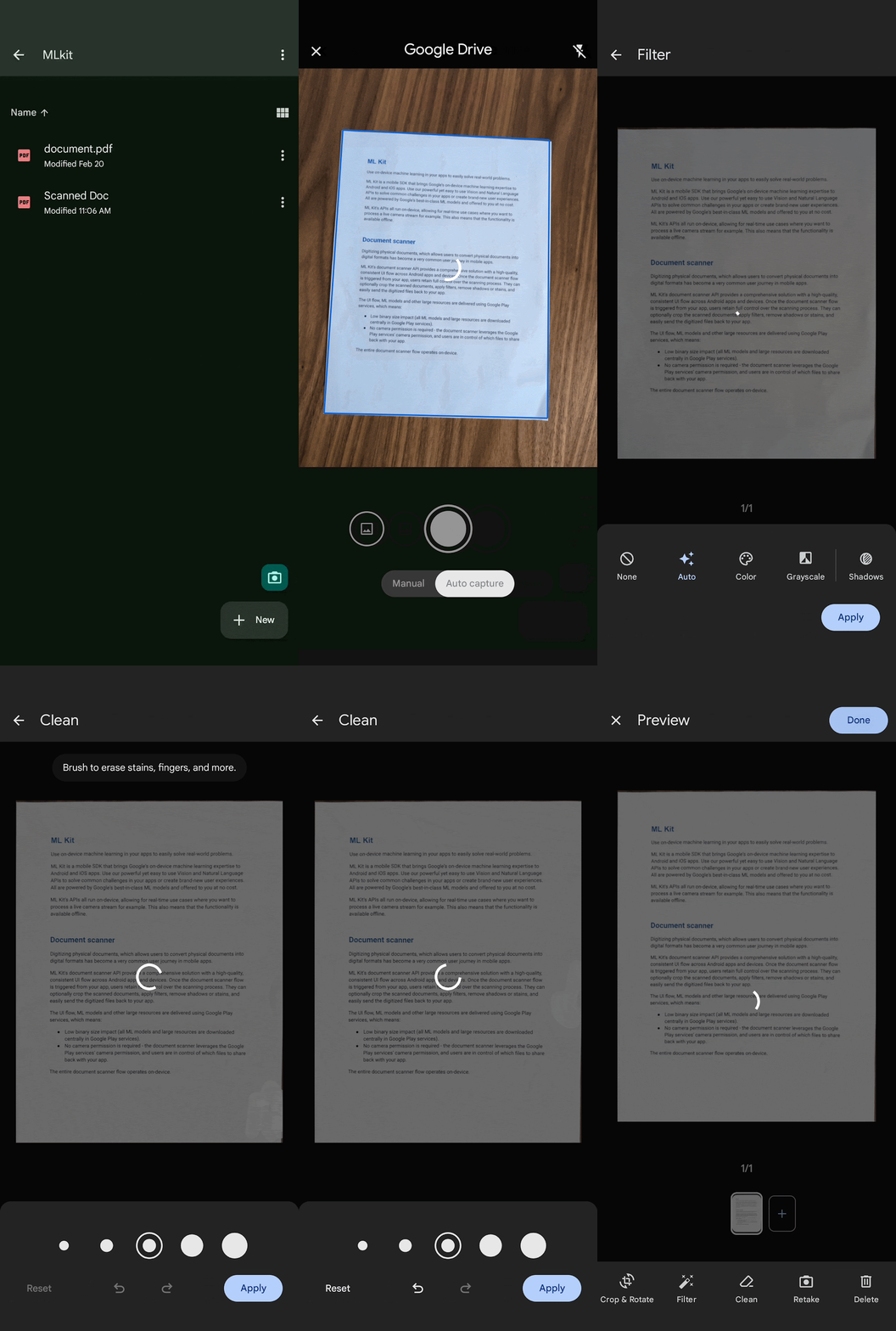
    • Flexible functionality allows users to crop scanned documents, apply filters, remove fingers, remove stains and other blemishes and send digitized files in PDF and JPEG formats back to your app.
    • On-device processing helps preserve privacy.
    • A complete solution eliminating the need for camera permission.

The ML Kit Document Scanner API is already used by Google Drive Android application and the Google Pixel Camera.

moving image showing ML Kit Document scanner API in action in  
Google Drive
ML Kit Document scanner API in action in Google Drive

Get started

The ML Kit Document Scanner API requires Android API level 21 or above. The models, scanning logic, and UI flow are dynamically downloaded via Google Play services so the ML Kit Document Scanner API has a minimal impact on your app size.

To integrate it in your app, start by configuring the scanner options and getting a scanner client:

val options = GmsDocumentScannerOptions.Builder()
    .setGalleryImportAllowed(false)
    .setPageLimit(2)
    .setResultFormats(RESULT_FORMAT_JPEG, RESULT_FORMAT_PDF)
    .setScannerMode(SCANNER_MODE_FULL)
    .build()
val scanner = GmsDocumentScanning.getClient(options)

Then register an ActivityResultCallback to receive the scanning results:

val scannerLauncher = registerForActivityResult(StartIntentSenderForResult()) {
  result -> {
    if (result.resultCode == RESULT_OK) {
      val result =
        GmsDocumentScanningResult.fromActivityResultIntent(result.data)
      result.getPages()?.let { pages ->
        for (page in pages) {
          val imageUri = page.getImageUri()
        }
      }
      result.getPdf()?.let { pdf ->
        val pdfUri = pdf.getUri()
        val pageCount = pdf.getPageCount()
      }
    }
  }
}

Finally launch the document scanner activity:

scanner.getStartScanIntent(activity)
  .addOnSuccessListener { intentSender ->   
    scannescannerrLauncher.launch(IntentSenderRequest.Builder(intentSender).build())
  }
  .addOnFailureListener { ... }

To get started with the ML Kit Document Scanner API, visit the documentation. We can’t wait to see what you’ll build with it!

Graph neural networks in TensorFlow

Objects and their relationships are ubiquitous in the world around us, and relationships can be as important to understanding an object as its own attributes viewed in isolation — take for example transportation networks, production networks, knowledge graphs, or social networks. Discrete mathematics and computer science have a long history of formalizing such networks as graphs, consisting of nodes connected by edges in various irregular ways. Yet most machine learning (ML) algorithms allow only for regular and uniform relations between input objects, such as a grid of pixels, a sequence of words, or no relation at all.

Graph neural networks, or GNNs for short, have emerged as a powerful technique to leverage both the graph’s connectivity (as in the older algorithms DeepWalk and Node2Vec) and the input features on the various nodes and edges. GNNs can make predictions for graphs as a whole (Does this molecule react in a certain way?), for individual nodes (What’s the topic of this document, given its citations?) or for potential edges (Is this product likely to be purchased together with that product?). Apart from making predictions about graphs, GNNs are a powerful tool used to bridge the chasm to more typical neural network use cases. They encode a graph's discrete, relational information in a continuous way so that it can be included naturally in another deep learning system.

We are excited to announce the release of TensorFlow GNN 1.0 (TF-GNN), a production-tested library for building GNNs at large scales. It supports both modeling and training in TensorFlow as well as the extraction of input graphs from huge data stores. TF-GNN is built from the ground up for heterogeneous graphs, where types of objects and relations are represented by distinct sets of nodes and edges. Real-world objects and their relations occur in distinct types, and TF-GNN's heterogeneous focus makes it natural to represent them.

Inside TensorFlow, such graphs are represented by objects of type tfgnn.GraphTensor. This is a composite tensor type (a collection of tensors in one Python class) accepted as a first-class citizen in tf.data.Dataset, tf.function, etc. It stores both the graph structure and its features attached to nodes, edges and the graph as a whole. Trainable transformations of GraphTensors can be defined as Layers objects in the high-level Keras API, or directly using the tfgnn.GraphTensor primitive.


GNNs: Making predictions for an object in context

For illustration, let’s look at one typical application of TF-GNN: predicting a property of a certain type of node in a graph defined by cross-referencing tables of a huge database. For example, a citation database of Computer Science (CS) arXiv papers with one-to-many cites and many-to-one cited relationships where we would like to predict the subject area of each paper.

Like most neural networks, a GNN is trained on a dataset of many labeled examples (~millions), but each training step consists only of a much smaller batch of training examples (say, hundreds). To scale to millions, the GNN gets trained on a stream of reasonably small subgraphs from the underlying graph. Each subgraph contains enough of the original data to compute the GNN result for the labeled node at its center and train the model. This process — typically referred to as subgraph sampling — is extremely consequential for GNN training. Most existing tooling accomplishes sampling in a batch way, producing static subgraphs for training. TF-GNN provides tooling to improve on this by sampling dynamically and interactively.

Pictured, the process of subgraph sampling where small, tractable subgraphs are sampled from a larger graph to create input examples for GNN training.

TF-GNN 1.0 debuts a flexible Python API to configure dynamic or batch subgraph sampling at all relevant scales: interactively in a Colab notebook (like this one), for efficient sampling of a small dataset stored in the main memory of a single training host, or distributed by Apache Beam for huge datasets stored on a network filesystem (up to hundreds of millions of nodes and billions of edges). For details, please refer to our user guides for in-memory and beam-based sampling, respectively.

On those same sampled subgraphs, the GNN’s task is to compute a hidden (or latent) state at the root node; the hidden state aggregates and encodes the relevant information of the root node's neighborhood. One classical approach is message-passing neural networks. In each round of message passing, nodes receive messages from their neighbors along incoming edges and update their own hidden state from them. After n rounds, the hidden state of the root node reflects the aggregate information from all nodes within n edges (pictured below for n = 2). The messages and the new hidden states are computed by hidden layers of the neural network. In a heterogeneous graph, it often makes sense to use separately trained hidden layers for the different types of nodes and edges

Pictured, a simple message-passing neural network where, at each step, the node state is propagated from outer to inner nodes where it is pooled to compute new node states. Once the root node is reached, a final prediction can be made.

The training setup is completed by placing an output layer on top of the GNN’s hidden state for the labeled nodes, computing the loss (to measure the prediction error), and updating model weights by backpropagation, as usual in any neural network training.

Beyond supervised training (i.e., minimizing a loss defined by labels), GNNs can also be trained in an unsupervised way (i.e., without labels). This lets us compute a continuous representation (or embedding) of the discrete graph structure of nodes and their features. These representations are then typically utilized in other ML systems. In this way, the discrete, relational information encoded by a graph can be included in more typical neural network use cases. TF-GNN supports a fine-grained specification of unsupervised objectives for heterogeneous graphs.


Building GNN architectures

The TF-GNN library supports building and training GNNs at various levels of abstraction.

At the highest level, users can take any of the predefined models bundled with the library that are expressed in Keras layers. Besides a small collection of models from the research literature, TF-GNN comes with a highly configurable model template that provides a curated selection of modeling choices that we have found to provide strong baselines on many of our in-house problems. The templates implement GNN layers; users need only to initialize the Keras layers.

At the lowest level, users can write a GNN model from scratch in terms of primitives for passing data around the graph, such as broadcasting data from a node to all its outgoing edges or pooling data into a node from all its incoming edges (e.g., computing the sum of incoming messages). TF-GNN’s graph data model treats nodes, edges and whole input graphs equally when it comes to features or hidden states, making it straightforward to express not only node-centric models like the MPNN discussed above but also more general forms of GraphNets. This can, but need not, be done with Keras as a modeling framework on the top of core TensorFlow. For more details, and intermediate levels of modeling, see the TF-GNN user guide and model collection.


Training orchestration

While advanced users are free to do custom model training, the TF-GNN Runner also provides a succinct way to orchestrate the training of Keras models in the common cases. A simple invocation may look like this:

The Runner provides ready-to-use solutions for ML pains like distributed training and tfgnn.GraphTensor padding for fixed shapes on Cloud TPUs. Beyond training on a single task (as shown above), it supports joint training on multiple (two or more) tasks in concert. For example, unsupervised tasks can be mixed with supervised ones to inform a final continuous representation (or embedding) with application specific inductive biases. Callers only need substitute the task argument with a mapping of tasks:

Additionally, the TF-GNN Runner also includes an implementation of integrated gradients for use in model attribution. Integrated gradients output is a GraphTensor with the same connectivity as the observed GraphTensor but its features replaced with gradient values where larger values contribute more than smaller values in the GNN prediction. Users can inspect gradient values to see which features their GNN uses the most.


Conclusion

In short, we hope TF-GNN will be useful to advance the application of GNNs in TensorFlow at scale and fuel further innovation in the field. If you’re curious to find out more, please try our Colab demo with the popular OGBN-MAG benchmark (in your browser, no installation required), browse the rest of our user guides and Colabs, or take a look at our paper.


Acknowledgements

The TF-GNN release 1.0 was developed by a collaboration between Google Research: Sami Abu-El-Haija, Neslihan Bulut, Bahar Fatemi, Johannes Gasteiger, Pedro Gonnet, Jonathan Halcrow, Liangze Jiang, Silvio Lattanzi, Brandon Mayer, Vahab Mirrokni, Bryan Perozzi, Anton Tsitsulin, Dustin Zelle, Google Core ML: Arno Eigenwillig, Oleksandr Ferludin, Parth Kothari, Mihir Paradkar, Jan Pfeifer, Rachael Tamakloe, and Google DeepMind: Alvaro Sanchez-Gonzalez and Lisa Wang.

Source: Google AI Blog


A decoder-only foundation model for time-series forecasting

Time-series forecasting is ubiquitous in various domains, such as retail, finance, manufacturing, healthcare and natural sciences. In retail use cases, for example, it has been observed that improving demand forecasting accuracy can meaningfully reduce inventory costs and increase revenue. Deep learning (DL) models have emerged as a popular approach for forecasting rich, multivariate, time-series data because they have proven to perform well in a variety of settings (e.g., DL models dominated the M5 competition leaderboard).

At the same time, there has been rapid progress in large foundation language models used for natural language processing (NLP) tasks, such as translation, retrieval-augmented generation, and code completion. These models are trained on massive amounts of textual data derived from a variety of sources like common crawl and open-source code that allows them to identify patterns in languages. This makes them very powerful zero-shot tools; for instance, when paired with retrieval, they can answer questions about and summarize current events.

Despite DL-based forecasters largely outperforming traditional methods and progress being made in reducing training and inference costs, they face challenges: most DL architectures require long and involved training and validation cycles before a customer can test the model on a new time-series. A foundation model for time-series forecasting, in contrast, can provide decent out-of-the-box forecasts on unseen time-series data with no additional training, enabling users to focus on refining forecasts for the actual downstream task like retail demand planning.

To that end, in “A decoder-only foundation model for time-series forecasting”, we introduce TimesFM, a single forecasting model pre-trained on a large time-series corpus of 100 billion real world time-points. Compared to the latest large language models (LLMs), TimesFM is much smaller (200M parameters), yet we show that even at such scales, its zero-shot performance on a variety of unseen datasets of different domains and temporal granularities come close to the state-of-the-art supervised approaches trained explicitly on these datasets. Later this year we plan to make this model available for external customers in Google Cloud Vertex AI.


A decoder-only foundation model for time-series forecasting

LLMs are usually trained in a decoder-only fashion that involves three steps. First, text is broken down into subwords called tokens. Then, the tokens are fed into stacked causal transformer layers that produce an output corresponding to each input token (it cannot attend to future tokens). Finally, the output corresponding to the i-th token summarizes all the information from previous tokens and predicts the (i+1)-th token. During inference, the LLM generates the output one token at a time. For example, when prompted with “What is the capital of France?”, it might generate the token “The”, then condition on “What is the capital of France? The” to generate the next token “capital” and so on until it generates the complete answer: “The capital of France is Paris”.

A foundation model for time-series forecasting should adapt to variable context (what we observe) and horizon (what we query the model to forecast) lengths, while having enough capacity to encode all patterns from a large pretraining dataset. Similar to LLMs, we use stacked transformer layers (self-attention and feedforward layers) as the main building blocks for the TimesFM model. In the context of time-series forecasting, we treat a patch (a group of contiguous time-points) as a token that was popularized by a recent long-horizon forecasting work. The task then is to forecast the (i+1)-th patch of time-points given the i-th output at the end of the stacked transformer layers.

However, there are several key differences from language models. Firstly, we need a multilayer perceptron block with residual connections to convert a patch of time-series into a token that can be input to the transformer layers along with positional encodings (PE). For that, we use a residual block similar to our prior work in long-horizon forecasting. Secondly, at the other end, an output token from the stacked transformer can be used to predict a longer length of subsequent time-points than the input patch length, i.e., the output patch length can be larger than the input patch length.

Consider a time-series of length 512 time-points being used to train a TimesFM model with input patch length 32 and output patch length 128. During training, the model is simultaneously trained to use the first 32 time-points to forecast the next 128 time-points, the first 64 time-points to forecast time-points 65 to 192, the first 96 time-points to forecast time-points 97 to 224 and so on. During inference, suppose the model is given a new time-series of length 256 and tasked with forecasting the next 256 time-points into the future. The model will first generate the future predictions for time-points 257 to 384, then condition on the initial 256 length input plus the generated output to generate time-points 385 to 512. On the other hand, if in our model the output patch length was equal to the input patch length of 32 then for the same task we would have to go through eight generation steps instead of just the two above. This increases the chances of more errors accumulating and therefore, in practice, we see that a longer output patch length yields better performance for long-horizon forecasting

TimesFM architecture.


Pretraining data

Just like LLMs get better with more tokens, TimesFM requires a large volume of legitimate time series data to learn and improve. We have spent a great amount of time creating and assessing our training datasets, and the following is what we have found works best:

Synthetic data helps with the basics. Meaningful synthetic time-series data can be generated using statistical models or physical simulations. These basic temporal patterns can teach the model the grammar of time series forecasting.

Real-world data adds real-world flavor. We comb through available public time series datasets, and selectively put together a large corpus of 100 billion time-points. Among these datasets there are Google Trends and Wikipedia Pageviews, which track what people are interested in, and that nicely mirrors trends and patterns in many other real-world time series. This helps TimesFM understand the bigger picture and generalize better when provided with domain-specific contexts not seen during training.


Zero-shot evaluation results

We evaluate TimesFM zero-shot on data not seen during training using popular time-series benchmarks. We observe that TimesFM performs better than most statistical methods like ARIMA, ETS and can match or outperform powerful DL models like DeepAR, PatchTST that have been explicitly trained on the target time-series.

We used the Monash Forecasting Archive to evaluate TimesFM’s out-of-the-box performance. This archive contains tens of thousands of time-series from various domains like traffic, weather, and demand forecasting covering frequencies ranging from few minutes to yearly data. Following existing literature, we inspect the mean absolute error (MAE) appropriately scaled so that it can be averaged across the datasets. We see that zero-shot (ZS) TimesFM is better than most supervised approaches, including recent deep learning models. We also compare TimesFM to GPT-3.5 for forecasting using a specific prompting technique proposed by llmtime(ZS). We demonstrate that TimesFM performs better than llmtime(ZS) despite being orders of magnitude smaller.

Scaled MAE (the lower the better) of TimesFM(ZS) against other supervised and zero-shot approaches on Monash datasets.

Most of the Monash datasets are short or medium horizon, i.e., the prediction length is not too long. We also test TimesFM on popular benchmarks for long horizon forecasting against a recent state-of-the-art baseline PatchTST (and other long-horizon forecasting baselines). In the next figure, we plot the MAE on ETT datasets for the task of predicting 96 and 192 time-points into the future. The metric has been calculated on the last test window of each dataset (as done by the llmtime paper). We see that TimesFM not only surpasses the performance of llmtime(ZS) but also matches that of the supervised PatchTST model explicitly trained on the respective datasets.

Last window MAE (the lower the better) of TimesFM(ZS) against llmtime(ZS) and long-horizon forecasting baselines on ETT datasets.


Conclusion

We train a decoder-only foundation model for time-series forecasting using a large pretraining corpus of 100B real world time-points, the majority of which was search interest time-series data derived from Google Trends and pageviews from Wikipedia. We show that even a relatively small 200M parameter pretrained model that uses our TimesFM architecture displays impressive zero-shot performance on a variety of public benchmarks from different domains and granularities.


Acknowledgements

This work is the result of a collaboration between several individuals across Google Research and Google Cloud, including (in alphabetical order): Abhimanyu Das, Weihao Kong, Andrew Leach, Mike Lawrence, Alex Martin, Rajat Sen, Yang Yang and Yichen Zhou.

Source: Google AI Blog