 Posted by Sharbani Roy – Senior Director, Product Management, Google

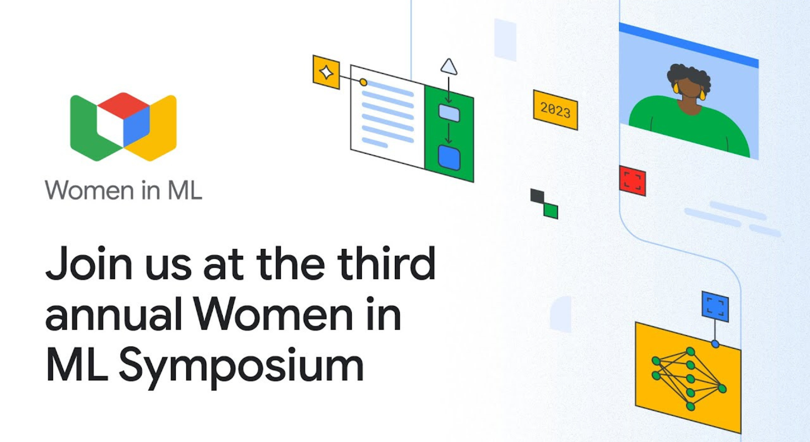
We’re back with the third annual Women in Machine Learning Symposium on December 7, 2023!
Join us virtually from 9:30 am to 1:00 pm PT for an immersive and insightful set of deep dives for every level of Machine Learning experience.
The Women in ML Symposium is an inclusive event for anyone passionate about the transformative fields of Machine Learning (ML) and Artificial Intelligence (AI). Meet this year’s women in ML as they uncover practical applications across multiple industries and discuss the latest advancements in frameworks, generative AI, and more.
Joana Carrasqueira, presenter for “Enabling Anyone to Build with Google AI”
Joana is a Developer Relations Lead for AI/ML at Google and her mission is to empower individuals and organizations to harness the power of AI to address real-world challenges.
She is a business leader with a track record of bringing strategic vision and global cross-functional programs to life. She’s also the creator of Google’s Women in ML program and flagship symposium, a pioneering initiative that has equipped thousands of developers with knowledge and skills in AI/ML.
Prior to Google, she worked at the Silicon Valley Innovation Center on innovation consulting for Forbes top500, startups and Venture Capital firms. Served as Education Manager at the International Pharmaceutical Federation, working closely with WHO, UNESCO, the United Nations and started her career at the Portuguese Pharmaceutical Society.
Joana holds an MBA from IE Business School, a Master in Pharmaceutical Sciences and a Leadership Certificate from U.C. Berkeley in California.
Sharbani Roy, presenter for “What’s New in Machine Learning?”
Sharbani is Sr. Director in Google’s Core Machine Learning group.
Before joining Google, Sharbani led engineering and product teams in Amazon Alexa, focused on media streaming, real-time communication, and applied ML (e.g., NLU, CV, and AR) for 1P/3P developers and end consumers.
Sharbani holds degrees in physics and mathematics from the University of Chicago and an MBA from Stanford University, and lives in Seattle with her husband and three children.
Eve Phillips, presenter for “Future of Frameworks: Navigate the OSS Landscape"
Eve is a Director of Product Management at Google.
Currently, Eve leads the ML Frameworks product team, which includes responsibility for TensorFlow, JAX and Keras. Previously, she led product teams within Google for Clinicians and ChromeOS. Prior to Google, she served as CEO of Empower Interactive, delivering tech-enabled behavioral health.
Earlier, she held roles in leading technology companies and investors including Trilogy, Microsoft, and Greylock.
Eve earned a BS and M.Eng in EECS from MIT and an MBA from Stanford.
Meenu Gaba, presenter for “Data-Centric AI: A New Paradigm"

Meenu leads the Machine Learning infrastructure team at Google, with a mission to power AI innovation with world-class ML infrastructure and services.
She is a technology leader with years of experience launching new products and growing small teams into mature scalable, multi-tiered organizations that are poised to deliver high quality products. Meenu enjoys fast-paced, dynamic, highly iterative/innovative environments and has lots of experience in balancing these disciplines while fostering a people-first culture and forming solid grounds for cross-functional relationships.
Meenu holds a Master's degree in Computer Science. In her free time, she enjoys hiking, solving crosswords, and watching movies.
Kelly Shaefer, presenter for “Maximize Your Data Exploration”

Kelly leads product teams at Google Labs, building both entirely new AI products and AI-enabled features into Google's largest existing products.
In the past, she led the Growth team for Google Workspace, including Gmail, Drive, Docs, and many more.
Outside of Google, she led the Enterprise product team at Stripe and was the P&L owner for Stripe's multi-billion dollar Payments area.
Kelly has an undergraduate degree from Wharton at UPenn, and an MBA from Harvard Business School.
Divyashree Sreepathihalli, presenter for “Keras: Shortcut to AI Mastery”
Divya is a talented machine learning software engineer who is currently a part of the Keras team at Google.
In this role, she specializes in developing Keras core modeling APIs and KerasCV to improve the functionality of the software.
Prior to joining Google, Divya worked as a Deep Learning Scientist for Zazu Sensor, a startup group in Intel's Emerging Growth Incubation (EGI) group. Her work there focused on computer vision and deep learning algorithm development for object detection and tracking, resulting in significant advancements for the startup.
Divya completed her Masters in Computer Engineering from Texas A&M University where she focused on Artificial intelligence in 2017.
Na Li, presenter for “Prototype ML with Visual Blocks”
Na Li is a software engineer manager from Google CoreML.
She leads a team to build developer tools to support ML development journey, from prototyping to model visualization and benchmarking.
Prior to Google, she was a research scientist at Harvard, working in HCI domain.
Throughout her career, Na strives to make ML accessible for everyone.
Zoe Wang, presenter for “Deploying ML Models to Mobile Devices”

Zoe is a technical program manager at Google.
Her career has been focused on Machine Learning (ML) productionization.
Currently she works with her team bringing ML models to mobile devices that power some of AI features for Pixel and other edge devices.
Prior to Google, Zoe worked at Meta on ML Platforms for end-to-end ML lifecycles.
Yvonne Li, presenter for “New GenAI Products and Solutions on Google Cloud”

Yvonne Li is a software engineer on the Duet Platform team at Google, where she focuses on improving the quality of generative AI models.
As a machine learning engineer and developer advocate at IBM, she designed and developed language models and curated open source datasets.
She has over 3 years of experience in the big tech industry, and is passionate about using machine learning to solve real-world problems.
Yvonne is the author of two Coursera courses: Data Analysis with R, and, Data Visualization with R.
Nithya Natesan, presenter for “AI-powered Infrastructure: Cloud TPUs”

Nithya Natesan is a Group Product Manager in the Cloud ML Accelerators team focussing on GPU / TPU offerings for Google Cloud.
Prior to Google, she was head of product management at NVIDIA, launching several products like DGX Cloud, Base Command Platform.
She has ~14 years of experience in hyper convergence Data Center software products, with recent focus on ML / AI Infra and Platform products. She is passionate about building rock solid PM teams, and shipping high quality usable ML / AI products.
Nithya has also won industry accolades namely WomenImpactTech 2023.
Andrada Vulpe, presenter for “Community Matters: 8 Reasons Why You Should Be Involved with Kaggle”

Andrada is a Data Scientist at Endava, a Notebooks Grandmaster on Kaggle, a Dev Expert at Weights and Biases and a proud Z by HP Data Science Global Ambassador.
She is highly passionate about Python, R, Machine and Deep Learning, powerful visualizations and everything in between.
Andrada finished her MSc in Data Science and Analytics in the UK and won 2 Kaggle Analytics competitions.
Jeehae Lee, presenter for “From Recovering Pro Golfer to AI Entrepreneur”

Jeehae Lee is a golf industry executive who has worked to create and build transformational sports technology businesses.
As the Co-Founder & CEO of Sportsbox AI, Jeehae is currently developing products using AI-enabled 3D motion analysis technology that will help participants of various sports and fitness activities learn and improve their skills.
Before founding Sportsbox, she spent five years between 2015 and 2020 at Topgolf Entertainment Group, leading strategy and new business development for various divisions including Toptracer. Between 2012 and 2013, she was at global sports and entertainment marketing agency, IMG, representing professional golfer icon Michelle Wie West. Prior to her career in sports business, she played professional golf at the highest level in the sport, competing on the LPGA tour for three years between 2009 and 2011.
Jeehae is a proud graduate of Phillips Academy in Andover, MA, and has a BA in Economics from Yale and an MBA from The Wharton School at University of Pennsylvania.
Jingwan (Cynthia) Lu, panelist for “The Impact of Generative AI in Different Industries”
Cynthia is a senior director from Adobe leading an applied research organization focusing on developing the Adobe Firefly family of GenAI models built from the ground up.
Her team started training Adobe’s first large-scale foundational model and helped rally together the rest of the company to roll out a new web-based product called Firefly featuring the image generation model as the first step in early 2023.
The same technology and its extension power Adobe Photoshop’s Generative Fill and Generative Expand features giving users intelligent image inpainting and outpainting experience. Time recognizes Adobe Photoshop Generative Fill and Generative Expand as best inventions of 2023 in the AI category.
Before Firefly, Jingwan was a computer vision research scientist and team lead who pioneered and led a large group effort to explore early generative models such as GANs within Adobe.
Wei Xiao, panelist for “The Impact of Generative AI in Different Industries”
Wei is the Director of Developer Relations at NVIDIA for the Middle East, Africa, and emerging regions. Her primary focus is to drive AI and accelerated computing integration within the ecosystem.
Before assuming her current role, Wei Xiao headed Ecosystem Engineering and Evangelism teams at both ARM and Samsung Semiconductor.
In addition to her professional endeavors, Wei dedicates her free time to teaching AI courses at the Graduate School of Computer Science at Santa Clara University.
Priya Mathur, panelist for “The Impact of Generative AI in Different Industries”

Priya is a Staff Data Science Manager at Google and she is the founder of Sparkle – GenAI Data Analyst.
At Google, she leads Data Science for Home Platform Monetization and GenAI efforts for DSPA.
Previously at Groupon, she led Data Science for App Push Notifications and TV Ads.
Katherine Chou, panelist for “The Impact of Generative AI in Different Industries”
Katherine is the Senior Director of Research and Innovations at Google with a specific focus on nurturing scientific and technical breakthroughs that can lead to global impact for science, health, climate, and advancement of platform technologies for our developers and researchers.
Katherine is focused on improving the availability and accuracy of healthcare using machine learning. She is a serial intrapreneur, particularly interested in removing health inequities and improving health and well-being outcomes across all populations.
She previously developed products within Google[x] Labs for Life Sciences (now Verily) and co-founded Medical Brain (now “Health AI'') at Google. She also headed up global teams to develop partner solutions and establish developer ecosystems for Mobile Payments, Mobile Search, GeoCommerce, YouTube, and Android.
Outside of Google, she is a Board member and Program Chair of Lewa Wildlife Conservancy, a Scientific Advisor to the ARCS Foundation, a fellow of the Zoological Society of London, and collaborates with other wildlife NGOs and the Cambridge Business Sustainability Programme in applying the Silicon Valley innovation mindset to new areas.
Katherine holds a double major in Computer Science and Economics at Stanford University and an M.S. in CS specialized in graphics.
Jaimie Hwang, presenter for “Take Action, Learn More, Start Building with Google AI”
Jaimie Hwang is a global product marketing leader with over a decade of experience, specifically in AI/ML.
She has built and led global product marketing teams at a number of AI companies, including an award-winning computer vision startup and tech giant Amazon.
She specializes in executive thought leadership, product storytelling, and integrated GTM strategy. She is passionate about promoting AI technology that is built responsibly and solves real-world problems in a human-centric way.
Jaimie holds a BS in Journalism and Integrated Marketing and Communications from Northwestern University. She lives in Seattle, Washington.
Save your spot at WiML Symposium 2023
The Women in ML Symposium offers sessions for all expertise levels, from beginners to advanced practitioners. RSVP today to secure your spot and explore our comprehensive agenda. We can’t wait to see you there!


 Posted by