Tag Archives: machine learning

The Machine Learning Behind Android Smart Linkify


Earlier this week we launched Android 9 Pie, the latest release of Android that uses machine learning to make your phone simpler to use. One of the features in Android 9 is Smart Linkify, a new API that adds clickable links when certain types of entities are detected in text. This is useful when, for example, you receive an address from a friend in a messaging app and want to look it up on a map. With a Smart Linkify-annotated text, it’s a lot easier!
Smart Linkify is a new version of the existing Android Linkify API. It is powered by a small feed-forward neural network (500kB per language) with low latency (less than 20ms on Google Pixel phones) and small inference code (250kB), and uses essentially the same machine learning technology that powers Smart Text Selection (released as part of Android Oreo) to now also create links.

Smart Linkify is available as an open-source TextClassifier API in Android (as the generateLinks method). The models were trained using TensorFlow and exported to a custom inference library backed by TensorFlow Lite and FlatBuffers. The C++ inference library for the models is available as part of Android Open-Source framework here, and runs on each text selection and Smart Linkify API calls.

Finding Entities
Looking for phone numbers and postal addresses in text is a difficult problem. Not only are there many variations in how people write them, but it’s also often ambiguous what type of entity is being represented (e.g. “Confirmation number: 857-555-3556” is not a phone number even though it it takes a similar form to one). As a solution, we designed an inference algorithm with two small feedforward neural networks at its heart. This algorithm is general enough to perform all kinds of entity chunking beyond just addresses and phone numbers.

Overall, the system architecture is as follows: A given input text is first split into words (based on space separation), then all possible word subsequences of certain maximum length (15 words in our case) are generated, and for each candidate the scoring neural net assigns a value (between 0 and 1) based on whether it represents a valid entity:
For the given text string, the first network assigns low scores to non-entities and a high score for the candidate that correctly selects the whole phone number.
Next, the generated entities that overlap are removed, favoring the ones with the higher score over the conflicting ones with a lower score. Now, we have a set of entities, but still don’t know their types. So now the second neural network is used to classify the type of the entity, as either a phone number, address or in some cases, a non-entity.

In our example, the only non-conflicting entities are “And call 857 555 3556tomorrow.” (with “857 555 3556” classified as a phone number), and “And call 857 555 3556 tomorrow.” (with “And” classified as a non-entity).

Now that we have the only non-conflicting entities, “And call 857 555 3556 tomorrow.” (with “857 555 3556” classified as a phone number) and “And call 857 555 3556 tomorrow.” (with “And” classified as a non-entity), we are easily able to underline them in the displayed text on the screen, and run the right app when clicked.

Textual Features
So far, we’ve given a general description of the way Smart Linkify locates and classifies entities in a string of text. Here, we go into more detail on how the text is processed and fed to the network.

The task of the networks, given an entity candidate in the input text, is to determine whether the entity is valid, and then to classify it. To do this, the networks need to know the context surrounding the entity (in addition to the text string of the entity itself). In machine learning this is done by representing these parts as separate features. Effectively, the input text is split into several parts that are fed to the network separately:
Given a candidate entity span, we extract: Left context: five words before the entity, Entity start: first three words of the entity, Entity end: last three words of the entity (they can be duplicated with the previous feature if they overlap, or padded if there are not that many), Right context: five words after the entity, Entity content: bag of words inside the entity and Entity length: size of the entity in number of words. They are then concatenated together and fed as an input to the neural network.
The feature extraction operates with words, and we use character n-grams and a capitalization feature to represent the individual words as real vectors suitable as an input of the neural network:
  • Character N-grams. Instead of using the standard word embedding technique for representing words, which keeps a separate vector for each word in the model and thus would be infeasible for mobile devices because of their large storage size, we use the hashed charactergram embedding. This technique represents the word as a set of all character subsequences of certain length. We use lengths 1 to 5. These strings are additionally hashed and mapped to a fixed number of buckets (see here for more details on the technique). As a result, the final model only stores vectors for each of the hash buckets, not each word/character subsequence, and can be kept small. The embedding matrix for the hashed charactergrams that we use has 20,000 buckets and 12 dimensions.
  • A binary feature that indicates whether the word starts with a capital letter. This is important for the network to know because the capitalization in postal addresses is quite distinct, and helps the networks to discriminate.
A Training Dataset
There is no obvious dataset for this task on which we could readily train the networks, so we came up with a training algorithm that generates synthetic examples out of realistic pieces. Concretely, we gathered lists of addresses, phone numbers and named entities (like product, place and business names) and other random words from the Web (using Schema.org annotations), and use them to synthesize the training data for the neural networks. We take the entities as they are and generate random textual contexts around them (from the list of random words on Web). Additionally, we add phrases like “Confirmation number:” or “ID:” to the negative training data for phone numbers, to teach the network to suppress phone number matches in these contexts.

Making it Work
There are a number of additional techniques that we had to use for training the network and making a practical mobile deployment:
  • Quantizing the embedding matrix to 8 bits. We found that we could reduce the size of the model almost 4x without compromising the performance, by quantizing the embedding matrix values to 8-bit integers.
  • Sharing embedding matrices between the selection and classification networks. This brings almost no loss and makes the model 2x smaller.
  • Varying the size of the context before/after the entities. On mobile screens text is often short, with not enough context, so the network needs to be exposed to this during training as well.
  • Creating artificial negative examples out of the positive ones for the classification network. For example for the positive example: “call me 857 555-3556 today” with a label “phone” we generate “call me 857 555-3556 today” as a negative example with a label “other”. This teaches the classification network to be more precise about the entity span. Without doing this, the network would be merely a detector whether there is a phone number somewhere in the input, regardless of the span.
Internationalization is Important
The automatic data extraction we use makes it easier to train language-specific models. However, making them work for all languages is a challenge, requiring careful checking of language nuance by experts, as well as having an acceptable amount of training data. We found that having one model for all Latin-script languages works well (e.g. Czech, Polish, German, English), with individual models for each of Chinese, Japanese, Korean, Thai, Arabic and Russian. While Smark Linkify currently supports 16 languages, we are experimenting with models that support even more languages, which is especially challenging given the mobile model size constraints and trickiness with languages that do not split words on spaces.

Next Steps
While the technique described in this post enables the fast and accurate annotation of phone numbers and postal addresses in text, the recognition of flight numbers, date and time, or IBAN, is currently implemented with a more traditional technique using standard regular expressions. However, we are looking into creating ML models for date and time as well, particularly for recognizing informal relative date/time specifications prevalent in messaging context, like “next Thursday” or “in 3 weeks”.

The small model and binary size as well as low latency are very important for mobile deployment. The models and the code we developed are available open-source as part of Android framework. We believe that the architecture could extend to other on-device text annotation problems and we look forward to seeing new use cases from our developer community!

Source: Google AI Blog


Google Developers Launchpad introduces The Lever, sharing applied-Machine Learning best practices

Posted by Malika Cantor, Program Manager for Launchpad

The Lever is Google Developers Launchpad's new resource for sharing applied-Machine Learning (ML) content to help startups innovate and thrive. In partnership with experts and leaders across Google and Alphabet, The Lever is operated by Launchpad, Google's global startup acceleration program. The Lever will publish the Launchpad community's experiences of integrating ML into products, and will include case studies, insights from mentors, and best practices from both Google and global thought leaders.

Peter Norvig, Google ML Research Director, and Cassie Kozyrkov, Google Cloud Chief Decision Scientist, are editors of the publication. Hear from them and other Googlers on the importance of developing and sharing applied ML product and business methodologies:

Peter Norvig (Google ML Research, Director): "The software industry has had 50 years to perfect a methodology of software development. In Machine Learning, we've only had a few years, so companies need to pay more attention to the process in order to create products that are reliable, up-to-date, have good accuracy, and are respectful of their customers' private data."

Cassie Kozyrkov (Chief Decision Scientist, Google Cloud): "We live in exciting times where the contributions of researchers have finally made it possible for non-experts to do amazing things with Artificial Intelligence. Now that anyone can stand on the shoulders of giants, process-oriented avenues of inquiry around how to best apply ML are coming to the forefront. Among these is decision intelligence engineering: a new approach to ML, focusing on how to discover opportunities and build towards safe, effective, and reliable solutions. The world is poised to make data more useful than ever before!"

Clemens Mewald (Lead, Machine Learning X and TensorFlow X): "ML/AI has had a profound impact in many areas, but I would argue that we're still very early in this journey. Many applications of ML are incremental improvements on existing features and products. Video recommendations are more relevant, ads have become more targeted and personalized. However, as Sundar said, AI is more profound than electricity (or fire). Electricity enabled modern technology, computing, and the internet. What new products will be enabled by ML/AI? I am convinced that the right ML product methodologies will help lead the way to magical products that have previously been unthinkable."

We invite you to follow the publication, and actively comment on our blog posts to share your own experience and insights.

New AIY Edge TPU Boards

Posted by Billy Rutledge, Director of AIY Projects

Over the past year and a half, we've seen more than 200K people build, modify, and create with our Voice Kit and Vision Kit products. Today at Cloud Next we announced two new devices to help professional engineers build new products with on-device machine learning(ML) at their core: the AIY Edge TPU Dev Board and the AIY Edge TPU Accelerator. Both are powered by Google's Edge TPU and represent our first steps towards expanding AIY into a platform for experimentation with on-device ML.

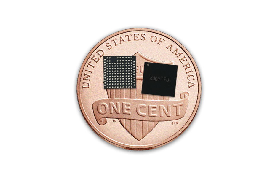
The Edge TPU is Google's purpose-built ASIC chip designed to run TensorFlow Lite ML models on your device. We've learned that performance-per-watt and performance-per-dollar are critical benchmarks when processing neural networks within a small footprint. The Edge TPU delivers both in a package that's smaller than the head of a penny. It can accelerate ML inferencing on device, or can pair with Google Cloud to create a full cloud-to-edge ML stack. In either configuration, by processing data directly on-device, a local ML accelerator increases privacy, removes the need for persistent connections, reduces latency, and allows for high performance using less power.

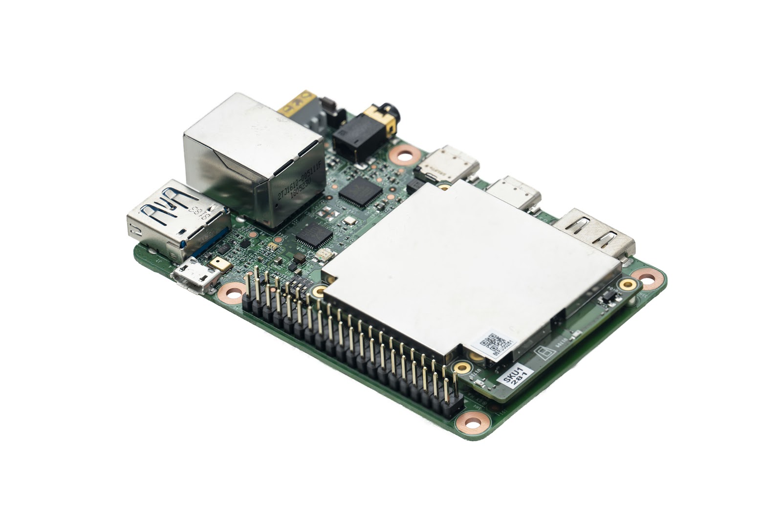
The AIY Edge TPU Dev Board is an all-in-one development board that allows you to prototype embedded systems that demand fast ML inferencing. The baseboard provides all the peripheral connections you need to effectively prototype your device — including a 40-pin GPIO header to integrate with various electrical components. The board also features a removable System-on-module (SOM) daughter board can be directly integrated into your own hardware once you're ready to scale.

The AIY Edge TPU Accelerator is a neural network coprocessor for your existing system. This small USB-C stick can connect to any Linux-based system to perform accelerated ML inferencing. The casing includes mounting holes for attachment to host boards such as a Raspberry Pi Zero or your custom device.

On-device ML is still in its early days, and we're excited to see how these two products can be applied to solve real world problems — such as increasing manufacturing equipment reliability, detecting quality control issues in products, tracking retail foot-traffic, building adaptive automotive sensing systems, and more applications that haven't been imagined yet.

Both devices will be available online this fall in the US with other countries to follow shortly.

For more product information visit g.co/aiy and sign up to be notified as products become available.

Machine Learning in Google BigQuery


Google BiqQuery allows interactive analysis of large datasets, making it easy for businesses to share meaningful insights and develop solutions based on customer analytics. However, many of the businesses that are using BigQuery aren’t using machine learning to help better understand the data they are generating. This is because data analysts, proficient in SQL, may not have the traditional data science background needed to apply machine learning techniques.

Today we’re announcing BigQuery ML, a capability inside BigQuery that allows data scientists and analysts to build and deploy machine learning models on massive structured or semi-structured datasets. BigQuery ML is a set of simple SQL language extensions which enables users to utilize popular ML capabilities, performing predictive analytics like forecasting sales and creating customer segmentations right at the source, where they already store their data. BigQuery ML additionally sets smart defaults automatically and takes care of data transformation, leading to a seamless and easy to use experience with great results.
When designing the BigQuery ML backend, the team was faced with a dilemma. Transferring large amounts of data from BigQuery servers to special-purpose servers running machine learning algorithms would be time-consuming and would incur an overhead in terms of security and privacy considerations. However, because the core components of gradient descent — an optimization method that is the workhorse of machine learning algorithms — can be implemented using common SQL operations*, we were able to repurpose the existing BigQuery SQL processing engine for BigQuery ML.

Since the BigQuery engine is designed to efficiently scan large datasets rather than randomly draw small samples from them, BigQuery ML is based on the standard (batch) variant of gradient descent rather than the stochastic version. And while stochastic gradient descent is far more common in today’s large-scale machine learning systems, the batch variant has numerous practical advantages.

For example, in-database machine learning systems based on stochastic gradient descent process examples one by one, and can perform poorly when the data is suboptimally ordered. But BigQuery data is often distributed on disk so as to optimize the performance of regular SQL queries, and continually redistributing the data to support stochastic machine learning algorithms would be computationally expensive. In contrast, batch gradient descent is insensitive to the ordering and partitioning of data on disk, thereby completely circumventing this problem. Also, batch methods can be combined with line search techniques from the classical optimization literature, leading to a learning algorithm that is more stable and requires less fine tuning. Using line search with stochastic methods is far trickier. Our implementation also includes support for regularization and preconditioning. For more details, please see our paper.

We hope that you’ll find BigQuery ML useful for many predictive analytics tasks. To try it, visit the BigQuery console and follow the user guide. Creating a model is as simple as:
CREATE MODEL dataset.model_name
OPTIONS(model_type=’linear_reg’, input_label_cols=[‘input_label’])
AS SELECT * FROM input_table;
In the future, we plan to further integrate our gradient descent implementation with BigQuery infrastructure to realize more performance gains. We’re also going to explore other machine learning algorithms that can be easily and efficiently implemented for large-scale problems by leveraging the power of BigQuery.

Acknowledgements
BigQuery ML is the result of a large collaboration across many teams at Google. Key contributors and sponsors include Hossein Ahmadi, Corinna Cortes, Grzegorz Czajkowski, Mingge Deng, Amir Hormati, Abhishek Kashyap, Jing Jing Long, Dan McClary, Chris Meyers, Girishkumar Sabhnani, Vivek Sharma, Jordan Tigani, Chad Verbowski, Jiaxun Wu and Lisa Yin.


* For example, a gradient vector can be computed using the SUM and GROUP BY operators, and the weights of a model can be updated using an INNER JOIN.

Source: Google AI Blog


The Machine Learning Crash Course (MLCC) Study Jam series comes to India

https://lh3.googleusercontent.com/2k1bZslf950IXN-bbAwpNQPq-ax9fQtVdTwdMm8vIXUL4FmaI0jybUMkJBpVH-Jae10t-UGM_He79bILjGPlTw=w1340-h646-c
Looking for an inroad into the world of Artificial Intelligence and Machine Learning? Now you can access practical -- and free -- training from Google experts


From helping farmers detect the onset of crop infections to enabling doctors diagnose the occurrence of diabetic blindness among millions, Artificial Intelligence is helping tackle challenges inventively across a range of sectors. At Google, we believe that AI has the potential to make apps and services more useful, while helping innovation among businesses and developers, be it in their own field or while taking on humanity’s big challenges.


In India the AI ecosystem is nascent but is developing rapidly. With companies of all sizes adopting AI in their solutions, there is a clear and present need for trained and technically-equipped developers to drive these AI-related challenges and projects. To help facilitate this, Google signed a Statement of Intent with NITI Aayog earlier this year to jointly work towards building the AI ecosystem in India.


One of the key initiatives of this collaboration is to train Indian developers in the field of Machine Learning. With this as the objective we are excited to  bring the Machine Learning Crash Course (MLCC) Study Jam series to India this July.


This course intends to improve developers’ technical proficiency in machine learning, enabling them to apply cutting-edge techniques to help take on a range of practical challenges.


About MLCC


MLCC is Google’s flagship machine learning course, initially created for Google engineers. This course was taken up by more than 18,000 Googlers, and was recently made publicly available.  MLCC provides exercises, interactive visualizations, and instructional videos that anyone can use to learn and practice ML concepts.


What does the course cover?


MLCC covers numerous machine learning fundamentals, from  basic concepts such as loss function and gradient descent, then building through more advanced theories like classification models and neural networks. The programming exercises include the basics of TensorFlow -- our open-source machine learning framework -- and also feature succinct videos from Google machine learning experts. Participants will be able to read short text lessons, and play with educational gadgets devised by Google’s instructional designers and engineers.


Who should take this (free!) course?


MLCC is intended for those who wish to learn about ML from a practical, applied perspective that will enable them to gain a deeper understanding of the power of TensorFlow, and incorporate best practices into their everyday projects. This course is ideally suited to developers with basic machine learning knowledge, who are keen to gain experience in ML and TensorFlow.


Posted by Chetan Krishnaswamy, Director - Public Policy, Google India

Self-Supervised Tracking via Video Colorization


Tracking objects in video is a fundamental problem in computer vision, essential to applications such as activity recognition, object interaction, or video stylization. However, teaching a machine to visually track objects is challenging partly because it requires large, labeled tracking datasets for training, which are impractical to annotate at scale.

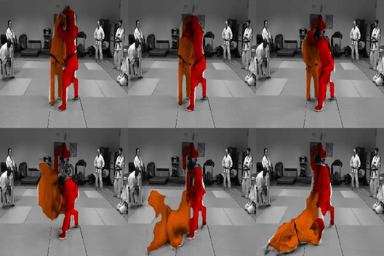
In “Tracking Emerges by Colorizing Videos”, we introduce a convolutional network that colorizes grayscale videos, but is constrained to copy colors from a single reference frame. In doing so, the network learns to visually track objects automatically without supervision. Importantly, although the model was never trained explicitly for tracking, it can follow multiple objects, track through occlusions, and remain robust over deformations without requiring any labeled training data.
Example tracking predictions on the publicly-available, academic dataset DAVIS 2017. After learning to colorize videos, a mechanism for tracking automatically emerges without supervision. We specify regions of interest (indicated by different colors) in the first frame, and our model propagates it forward without any additional learning or supervision.

Learning to Recolorize Video
Our hypothesis is that the temporal coherency of color provides excellent large-scale training data for teaching machines to track regions in video. Clearly, there are exceptions when color is not temporally coherent (such as lights turning on suddenly), but in general color is stable over time. Furthermore, most videos contain color, providing a scalable self-supervised learning signal. We decolor videos, and then add the colorization step because there may be multiple objects with the same color, but by colorizing we can teach machines to track specific objects or regions.

In order to train our system, we use videos from the Kinetics dataset, which is a large public collection of videos depicting everyday activities. We convert all video frames except the first frame into gray-scale, and train a convolutional network to predict the original colors in the subsequent frames. We expect the model to learn to follow regions in order to accurately recover the original colors. Our main observation is the need to follow objects for colorization will cause a model for object tracking to be automatically learned.
We illustrate the video recolorization task using video from the DAVIS 2017 dataset. The model receives as input one color frame and a gray-scale video, and predicts the colors for the rest of the video. The model learns to copy colors from the reference frame, which enables a mechanism for tracking to be learned without human supervision.
Learning to copy colors from the single reference frame requires the model to learn to internally point to the right region in order to copy the right colors. This forces the model to learn an explicit mechanism that we can use for tracking. To see how the video colorization model works, we show some predicted colorizations from videos in the Kinetics dataset below.

Examples of predicted colors from colorized reference frame applied to input video using the publicly-available Kinetics dataset.

Although the network is trained without ground-truth identities, our model learns to track any visual region specified in the first frame of a video. We can track outlined objects or a single point in the video. The only change we make is that, instead of propagating colors throughout the video, we now propagate labels representing the regions of interest.

Analyzing the Tracker
Since the model is trained on large amounts of unlabeled video, we want to gain insight into what the model learns. The videos below show a standard trick to visualize the embeddings learned by our model by projecting them down to three dimensions using Principal Component Analysis (PCA) and plotting it as an RGB movie. The results show that nearest neighbors in the learned embedding space tend to correspond to object identity, even over deformations and viewpoint changes.
Top Row: We show videos from the DAVIS 2017 dataset. Bottom Row: We visualize the internal embeddings from the colorization model. Similar embeddings will have a similar color in this visualization. This suggests the learned embedding is grouping pixels by object identity.

Tracking Pose
We found the model can also track human poses given key-points in an initial frame. We show results on the publicly-available, academic dataset JHMDB where we track a human joint skeleton.
Examples of using the model to track movements of the human skeleton. In this case the input was a human pose for the first frame and subsequent movement is automatically tracked. The model can track human poses even though it was never explicitly trained for this task.

While we do not yet outperform heavily supervised models, the colorization model learns to track video segments and human pose well enough to outperform the latest methods based on optical flow. Breaking down performance by motion type suggests that our model is a more robust tracker than optical flow for many natural complexities, such as dynamic backgrounds, fast motion, and occlusions. Please see the paper for details.

Future Work
Our results show that video colorization provides a signal that can be used for learning to track objects in videos without supervision. Moreover, we found that the failures from our system are correlated with failures to colorize the video, which suggests that further improving the video colorization model can advance progress in self-supervised tracking.

Acknowledgements
This project was only possible thanks to several collaborations at Google. The core team includes Abhinav Shrivastava, Alireza Fathi, Sergio Guadarrama and Kevin Murphy. We also thank David Ross, Bryan Seybold, Chen Sun and Rahul Sukthankar.

Source: Google AI Blog


Teaching Uncalibrated Robots to Visually Self-Adapt


People are remarkably proficient at manipulating objects without needing to adjust their viewpoint to a fixed or specific pose. This capability (referred to as visual motor integration) is learned during childhood from manipulating objects in various situations, and governed by a self-adaptation and mistake correction mechanism that uses rich sensory cues and vision as feedback. However, this capability is quite difficult for vision-based controllers in robotics, which until now have been built on a rigid setup for reading visual input data from a fixed mounted camera which should not be moved or repositioned at train and test time. The ability to quickly acquire visual motor control skills under large viewpoint variation would have substantial implications for autonomous robotic systems — for example, this capability would be particularly desirable for robots that can help rescue efforts in emergency or disaster zones.

In “Sim2Real Viewpoint Invariant Visual Servoing by Recurrent Control” presented at CVPR 2018 this week, we study a novel deep network architecture (consisting of two fully convolutional networks and a long short-term memory unit) that learns from a past history of actions and observations to self-calibrate. Using diverse simulated data consisting of demonstrated trajectories and reinforcement learning objectives, our visually-adaptive network is able to control a robotic arm to reach a diverse set of visually-indicated goals, from various viewpoints and independent of camera calibration.
Viewpoint invariant manipulation for visually indicated goal reaching with a physical robotic arm. We learn a single policy that can reach diverse goals from sensory input captured from drastically different camera viewpoints. First row shows the visually indicated goals.

The Challenge
Discovering how the controllable degrees of freedom (DoF) affect visual motion can be ambiguous and underspecified from a single image captured from an unknown viewpoint. Identifying the effect of actions on image-space motion and successfully performing the desired task requires a robust perception system augmented with the ability to maintain a memory of past actions. To be able to tackle this challenging problem, we had to address the following essential questions:
  • How can we make it feasible to provide the right amount of experience for the robot to learn the self-adaptation behavior based on pure visual observations that simulate a lifelong learning paradigm?
  • How can we design a model that integrates robust perception and self-adaptive control such that it can quickly transfer to unseen environments?
To do so, we devised a new manipulation task where a seven-DoF robot arm is provided with an image of an object and is directed to reach that particular goal amongst a set of distractor objects, while viewpoints change drastically from one trial to another. In doing so, we were able to simulate both the learning of complex behaviors and the transfer to unseen environments.
Visually indicated goal reaching task with a physical robotic arm and diverse camera viewpoints.
Harnessing Simulation to Learn Complex Behaviors
Collecting robot experience data is difficult and time-consuming. In a previous post, we showed how to scale up learning skills by distributing the data collection and trials to multiple robots. Although this approach expedited learning, it is still not feasibly extendable to learning complex behaviors such as visual self-calibration, where we need to expose robots to a huge space of various viewpoints. Instead, we opt to learn such complex behavior in simulation where we can collect unlimited robot trials and easily move the camera to various random viewpoints. In addition to fast data collection in simulation, we can also surpass hardware limitations requiring the installation of multiple cameras around a robot.
We use domain randomization technique to learn generalizable policies in simulation.
To learn visually robust features to transfer to unseen environments, we used a technique known as domain randomization (a.k.a. simulation randomization) introduced by Sadeghi & Levine (2017), that enables robots to learn vision-based policies entirely in simulation such that they can generalize to the real world. This technique was shown to work well for various robotic tasks such as indoor navigation, object localization, pick and placing, etc. In addition, to learn complex behaviors like self-calibration, we harnessed the simulation capabilities to generate synthetic demonstrations and combined reinforcement learning objectives to learn a robust controller for the robotic arm.
Viewpoint invariant manipulation for visually indicated goal reaching with a simulated seven-DoF robotic arm. We learn a single policy that can reach diverse goals from sensory input captured from dramatically different camera viewpoints.

Disentangling Perception from Control
To enable fast transfer to unseen environments, we devised a deep neural network that combines perception and control trained end-to-end simultaneously, while also allowing each to be learned independently if needed. This disentanglement between perception and control eases transfer to unseen environments, and makes the model both flexible and efficient in that each of its parts (i.e. 'perception' or 'control') can be independently adapted to new environments with small amounts of data. Additionally, while the control portion of the network was entirely trained by the simulated data, the perception part of our network was complemented by collecting a small amount of static images with object bounding boxes without needing to collect the whole action sequence trajectory with a physical robot. In practice, we fine-tuned the perception part of our network with only 76 object bounding boxes coming from 22 images.
Real-world robot and moving camera setup. First row shows the scene arrangements and the second row shows the visual sensory input to the robot.
Early Results
We tested the visually-adapted version of our network on a physical robot and on real objects with drastically different appearances than the ones used in simulation. Experiments were performed with both one or two objects on a table — “seen objects” (as labeled in the figure below) were used for visual adaptation using small collection of real static images, while “unseen objects” had not been seen during visual adaptation. During the test, the robot arm was directed to reach a visually indicated object from various viewpoints. For the two object experiments the second object was to "fool" the robotic arm. While the simulation-only network has good generalization capability (due to being trained with domain randomization technique), the very small amount of static visual data to visually adapt the controller boosted the performance, due to the flexible architecture of our network.
After adapting the visual features with the small amount of real images, performance was boosted by more than 10%. All used real objects are drastically different from the objects seen in simulation.
We believe that learning online visual self-adaptation is an important and yet challenging problem with the goal of learning generalizable policies for robots that can act in diverse and unstructured real world setup. Our approach can be extended to any sort of automatic self-calibration. See the video below for more information on this work.
Acknowledgements
This research was conducted by Fereshteh Sadeghi, Alexander Toshev, Eric Jang and Sergey Levine. We would also like to thank Erwin Coumans and Yunfei Bai for providing pybullet, and Vincent Vanhoucke for insightful discussions.


Source: Google AI Blog


How Can Neural Network Similarity Help Us Understand Training and Generalization?


In order to solve tasks, deep neural networks (DNNs) progressively transform input data into a sequence of complex representations (i.e., patterns of activations across individual neurons). Understanding these representations is critically important, not only for interpretability, but also so that we can more intelligently design machine learning systems. However, understanding these representations has proven quite difficult, especially when comparing representations across networks. In a previous post, we outlined the benefits of Canonical Correlation Analysis (CCA) as a tool for understanding and comparing the representations of convolutional neural networks (CNNs), showing that they converge in a bottom-up pattern, with early layers converging to their final representations before later layers over the course of training.

In “Insights on Representational Similarity in Neural Networks with Canonical Correlation” we develop this work further to provide new insights into the representational similarity of CNNs, including differences between networks which memorize (e.g., networks which can only classify images they have seen before) from those which generalize (e.g., networks which can correctly classify previously unseen images). Importantly, we also extend this method to provide insights into the dynamics of recurrent neural networks (RNNs), a class of models that are particularly useful for sequential data, such as language. Comparing RNNs is difficult in many of the same ways as CNNs, but RNNs present the additional challenge that their representations change over the course of a sequence. This makes CCA, with its helpful invariances, an ideal tool for studying RNNs in addition to CNNs. As such, we have additionally open sourced the code used for applying CCA on neural networks with the hope that will help the research community better understand network dynamics.

Representational Similarity of Memorizing and Generalizing CNNs
Ultimately, a machine learning system is only useful if it can generalize to new situations it has never seen before. Understanding the factors which differentiate between networks that generalize and those that don’t is therefore essential, and may lead to new methods to improve generalization performance. To investigate whether representational similarity is predictive of generalization, we studied two types of CNNs:
  • generalizing networks: CNNs trained on data with unmodified, accurate labels and which learn solutions which generalize to novel data.
  • memorizing networks: CNNs trained on datasets with randomized labels such that they must memorize the training data and cannot, by definition, generalize (as in Zhang et al., 2017).
We trained multiple instances of each network, differing only in the initial randomized values of the network weights and the order of the training data, and used a new weighted approach to calculate the CCA distance measure (see our paper for details) to compare the representations within each group of networks and between memorizing and generalizing networks.

We found that groups of different generalizing networks consistently converged to more similar representations (especially in later layers) than groups of memorizing networks (see figure below). At the softmax, which denotes the network’s ultimate prediction, the CCA distance for each group of generalizing and memorizing networks decreases substantially, as the networks in each separate group make similar predictions.
Groups of generalizing networks (blue) converge to more similar solutions than groups of memorizing networks (red). CCA distance was calculated between groups of networks trained on real CIFAR-10 labels (“Generalizing”) or randomized CIFAR-10 labels (“Memorizing”) and between pairs of memorizing and generalizing networks (“Inter”).
Perhaps most surprisingly, in later hidden layers, the representational distance between any given pair of memorizing networks was about the same as the representational distance between a memorizing and generalizing network (“Inter” in the plot above), despite the fact that these networks were trained on data with entirely different labels. Intuitively, this result suggests that while there are many different ways to memorize the training data (resulting in greater CCA distances), there are fewer ways to learn generalizable solutions. In future work, we plan to explore whether this insight can be used to regularize networks to learn more generalizable solutions.

Understanding the Training Dynamics of Recurrent Neural Networks
So far, we have only applied CCA to CNNs trained on image data. However, CCA can also be applied to calculate representational similarity in RNNs, both over the course of training and over the course of a sequence. Applying CCA to RNNs, we first asked whether the RNNs exhibit the same bottom-up convergence pattern we observed in our previous work for CNNs. To test this, we measured the CCA distance between the representation at each layer of the RNN over the course of training with its final representation at the end of training. We found that the CCA distance for layers closer to the input dropped earlier in training than for deeper layers, demonstrating that, like CNNs, RNNs also converge in a bottom-up pattern (see figure below).
Convergence dynamics for RNNs over the course of training exhibit bottom up convergence, as layers closer to the input converge to their final representations earlier in training than later layers. For example, layer 1 converges to its final representation earlier in training than layer 2 than layer 3 and so on. Epoch designates the number of times the model has seen the entire training set while different colors represent the convergence dynamics of different layers.
Additional findings in our paper show that wider networks (e.g., networks with more neurons at each layer) converge to more similar solutions than narrow networks. We also found that trained networks with identical structures but different learning rates converge to distinct clusters with similar performance, but highly dissimilar representations. We also apply CCA to RNN dynamics over the course of a single sequence, rather than simply over the course of training, providing some initial insights into the various factors which influence RNN representations over time.

Conclusions
These findings reinforce the utility of analyzing and comparing DNN representations in order to provide insights into network function, generalization, and convergence. However, there are still many open questions: in future work, we hope to uncover which aspects of the representation are conserved across networks, both in CNNs and RNNs, and whether these insights can be used to improve network performance. We encourage others to try out the code used for the paper to investigate what CCA can tell us about other neural networks!

Acknowledgements
Special thanks to Samy Bengio, who is a co-author on this work. We also thank Martin Wattenberg, Jascha Sohl-Dickstein and Jon Kleinberg for helpful comments.

Source: Google AI Blog


Keeping 2 billion Android devices safe with machine learning

Posted by Sai Deep Tetali, Software Engineer, Google Play Protect

At Google I/O 2017, we introduced Google Play Protect, our comprehensive set of security services for Android. While the name is new, the smarts powering Play Protect have protected Android users for years.

Google Play Protect's suite of mobile threat protections are built into more than 2 billion Android devices, automatically taking action in the background. We're constantly updating these protections so you don't have to think about security: it just happens. Our protections have been made even smarter by adding machine learning elements to Google Play Protect.

Security at scale

Google Play Protect provides in-the-moment protection from potentially harmful apps (PHAs), but Google's protections start earlier.

Before they're published in Google Play, all apps are rigorously analyzed by our security systems and Android security experts. Thanks to this process, Android devices that only download apps from Google Play are 9 times less likely to get a PHA than devices that download apps from other sources.

After you install an app, Google Play Protect continues its quest to keep your device safe by regularly scanning your device to make sure all apps are behaving properly. If it finds an app that is misbehaving, Google Play Protect either notifies you, or simply removes the harmful app to keep your device safe.

Our systems scan over 50 billion apps every day. To keep on the cutting edge of security, we look for new risks in a variety of ways, such as identifying specific code paths that signify bad behavior, investigating behavior patterns to correlate bad apps, and reviewing possible PHAs with our security experts.

In 2016, we added machine learning as a new detection mechanism and it soon became a critical part of our systems and tools.

Training our machines

In the most basic terms, machine learning means training a computer algorithm to recognize a behavior. To train the algorithm, we give it hundreds of thousands of examples of that behavior.

In the case of Google Play Protect, we are developing algorithms that learn which apps are "potentially harmful" and which are "safe." To learn about PHAs, the machine learning algorithms analyze our entire catalog of applications. Then our algorithms look at hundreds of signals combined with anonymized data to compare app behavior across the Android ecosystem to find PHAs. They look for behavior common to PHAs, such as apps that attempt to interact with other apps on the device, access or share your personal data, download something without your knowledge, connect to phishing websites, or bypass built-in security features.

When we find apps exhibit similar malicious behavior, we group them into families. Visualizing these PHA families helps us uncover apps that share similarities to known bad apps, but have yet remained under our radar.

After we identify a new PHA, we confirm our findings with expert security reviews. If the app in question is a PHA, Google Play Protect takes action on the app and then we feed information about that PHA back into our algorithms to help find more PHAs.

Doubling down on security

So far, our machine learning systems have successfully detected 60.3% of the malware identified by Google Play Protect in 2017.

In 2018, we're devoting a massive amount of computing power and talent to create, maintain and improve these machine learning algorithms. We're constantly leveraging artificial intelligence and our highly skilled researchers and engineers from all across Google to find new ways to keep Android devices safe and secure. In addition to our talented team, we work with the foremost security experts and researchers from around the world. These researchers contribute even more data and insights to keep Google Play Protect on the cutting edge of mobile security.

To check out Google Play Protect, open the Google Play app and tap Play Protect in the left panel.

Acknowledgements: This work was developed in joint collaboration with Google Play Protect, Safe Browsing and Play Abuse teams with contributions from Andrew Ahn, Hrishikesh Aradhye, Daniel Bali, Hongji Bao, Yajie Hu, Arthur Kaiser, Elena Kovakina, Salvador Mandujano, Melinda Miller, Rahul Mishra, Damien Octeau, Sebastian Porst, Chuangang Ren, Monirul Sharif, Sri Somanchi, Sai Deep Tetali, Zhikun Wang, and Mo Yu.