Author Archives: Research Blog

Moving Beyond Translation with the Universal Transformer


Last year we released the Transformer, a new machine learning model that showed remarkable success over existing algorithms for machine translation and other language understanding tasks. Before the Transformer, most neural network based approaches to machine translation relied on recurrent neural networks (RNNs) which operate sequentially (e.g. translating words in a sentence one-after-the-other) using recurrence (i.e. the output of each step feeds into the next). While RNNs are very powerful at modeling sequences, their sequential nature means that they are quite slow to train, as longer sentences need more processing steps, and their recurrent structure also makes them notoriously difficult to train properly.

In contrast to RNN-based approaches, the Transformer used no recurrence, instead processing all words or symbols in the sequence in parallel while making use of a self-attention mechanism to incorporate context from words farther away. By processing all words in parallel and letting each word attend to other words in the sentence over multiple processing steps, the Transformer was much faster to train than recurrent models. Remarkably, it also yielded much better translation results than RNNs. However, on smaller and more structured language understanding tasks, or even simple algorithmic tasks such as copying a string (e.g. to transform an input of “abc” to “abcabc”), the Transformer does not perform very well. In contrast, models that perform well on these tasks, like the Neural GPU and Neural Turing Machine, fail on large-scale language understanding tasks like translation.

In “Universal Transformers” we extend the standard Transformer to be computationally universal (Turing complete) using a novel, efficient flavor of parallel-in-time recurrence which yields stronger results across a wider range of tasks. We built on the parallel structure of the Transformer to retain its fast training speed, but we replaced the Transformer’s fixed stack of different transformation functions with several applications of a single, parallel-in-time recurrent transformation function (i.e. the same learned transformation function is applied to all symbols in parallel over multiple processing steps, where the output of each step feeds into the next). Crucially, where an RNN processes a sequence symbol-by-symbol (left to right), the Universal Transformer processes all symbols at the same time (like the Transformer), but then refines its interpretation of every symbol in parallel over a variable number of recurrent processing steps using self-attention. This parallel-in-time recurrence mechanism is both faster than the serial recurrence used in RNNs, and also makes the Universal Transformer more powerful than the standard feedforward Transformer.
The Universal Transformer repeatedly refines a series of vector representations (shown as h1 to hm) for each position of the sequence in parallel, by combining information from different positions using self-attention and applying a recurrent transition function. Arrows denote dependencies between operations.
At each step, information is communicated from each symbol (e.g. word in the sentence) to all other symbols using self-attention, just like in the original Transformer. However, now the number of times this transformation is applied to each symbol (i.e. the number of recurrent steps) can either be manually set ahead of time (e.g. to some fixed number or to the input length), or it can be decided dynamically by the Universal Transformer itself. To achieve the latter, we added an adaptive computation mechanism to each position which can allocate more processing steps to symbols that are more ambiguous or require more computations.

As an intuitive example of how this could be useful, consider the sentence “I arrived at the bank after crossing the river”. In this case, more context is required to infer the most likely meaning of the word “bank” compared to the less ambiguous meaning of “I” or “river”. When we encode this sentence using the standard Transformer, the same amount of computation is applied unconditionally to each word. However, the Universal Transformer’s adaptive mechanism allows the model to spend increased computation only on the more ambiguous words, e.g. to use more steps to integrate the additional contextual information needed to disambiguate the word “bank”, while spending potentially fewer steps on less ambiguous words.

At first it might seem restrictive to allow the Universal Transformer to only apply a single learned function repeatedly to process its input, especially when compared to the standard Transformer which learns to apply a fixed sequence of distinct functions. But learning how to apply a single function repeatedly means the number of applications (processing steps) can now be variable, and this is the crucial difference. Beyond allowing the Universal Transformer to apply more computation to more ambiguous symbols, as explained above, it further allows the model to scale the number of function applications with the overall size of the input (more steps for longer sequences), or to decide dynamically how often to apply the function to any given part of the input based on other characteristics learned during training. This makes the Universal Transformer more powerful in a theoretical sense, as it can effectively learn to apply different transformations to different parts of the input. This is something that the standard Transformer cannot do, as it consists of fixed stacks of learned Transformation blocks applied only once.

But while increased theoretical power is desirable, we also care about empirical performance. Our experiments confirm that Universal Transformers are indeed able to learn from examples how to copy and reverse strings and how to perform integer addition much better than a Transformer or an RNN (although not quite as well as Neural GPUs). Furthermore, on a diverse set of challenging language understanding tasks the Universal Transformer generalizes significantly better and achieves a new state of the art on the bAbI linguistic reasoning task and the challenging LAMBADA language modeling task. But perhaps of most interest is that the Universal Transformer also improves translation quality by 0.9 BLEU1 over a base Transformer with the same number of parameters, trained in the same way on the same training data. Putting things in perspective, this almost adds another 50% relative improvement on top of the previous 2.0 BLEU improvement that the original Transformer showed over earlier models when it was released last year.

The Universal Transformer thus closes the gap between practical sequence models competitive on large-scale language understanding tasks such as machine translation, and computationally universal models such as the Neural Turing Machine or the Neural GPU, which can be trained using gradient descent to perform arbitrary algorithmic tasks. We are enthusiastic about recent developments on parallel-in-time sequence models, and in addition to adding computational capacity and recurrence in processing depth, we hope that further improvements to the basic Universal Transformer presented here will help us build learning algorithms that are both more powerful, more data efficient, and that generalize beyond the current state-of-the-art.

If you’d like to try this for yourself, the code used to train and evaluate Universal Transformers can be found here in the open-source Tensor2Tensor repository.

Acknowledgements
This research was conducted by Mostafa Dehghani, Stephan Gouws, Oriol Vinyals, Jakob Uszkoreit, and Łukasz Kaiser. Additional thanks go to Ashish Vaswani, Douglas Eck, and David Dohan for their fruitful comments and inspiration.


1 A translation quality benchmark widely used in the machine translation community, computed on the standard WMT newstest2014 English to German translation test data set.

Source: Google AI Blog


The Machine Learning Behind Android Smart Linkify


Earlier this week we launched Android 9 Pie, the latest release of Android that uses machine learning to make your phone simpler to use. One of the features in Android 9 is Smart Linkify, a new API that adds clickable links when certain types of entities are detected in text. This is useful when, for example, you receive an address from a friend in a messaging app and want to look it up on a map. With a Smart Linkify-annotated text, it’s a lot easier!
Smart Linkify is a new version of the existing Android Linkify API. It is powered by a small feed-forward neural network (500kB per language) with low latency (less than 20ms on Google Pixel phones) and small inference code (250kB), and uses essentially the same machine learning technology that powers Smart Text Selection (released as part of Android Oreo) to now also create links.

Smart Linkify is available as an open-source TextClassifier API in Android (as the generateLinks method). The models were trained using TensorFlow and exported to a custom inference library backed by TensorFlow Lite and FlatBuffers. The C++ inference library for the models is available as part of Android Open-Source framework here, and runs on each text selection and Smart Linkify API calls.

Finding Entities
Looking for phone numbers and postal addresses in text is a difficult problem. Not only are there many variations in how people write them, but it’s also often ambiguous what type of entity is being represented (e.g. “Confirmation number: 857-555-3556” is not a phone number even though it it takes a similar form to one). As a solution, we designed an inference algorithm with two small feedforward neural networks at its heart. This algorithm is general enough to perform all kinds of entity chunking beyond just addresses and phone numbers.

Overall, the system architecture is as follows: A given input text is first split into words (based on space separation), then all possible word subsequences of certain maximum length (15 words in our case) are generated, and for each candidate the scoring neural net assigns a value (between 0 and 1) based on whether it represents a valid entity:
For the given text string, the first network assigns low scores to non-entities and a high score for the candidate that correctly selects the whole phone number.
Next, the generated entities that overlap are removed, favoring the ones with the higher score over the conflicting ones with a lower score. Now, we have a set of entities, but still don’t know their types. So now the second neural network is used to classify the type of the entity, as either a phone number, address or in some cases, a non-entity.

In our example, the only non-conflicting entities are “And call 857 555 3556tomorrow.” (with “857 555 3556” classified as a phone number), and “And call 857 555 3556 tomorrow.” (with “And” classified as a non-entity).

Now that we have the only non-conflicting entities, “And call 857 555 3556 tomorrow.” (with “857 555 3556” classified as a phone number) and “And call 857 555 3556 tomorrow.” (with “And” classified as a non-entity), we are easily able to underline them in the displayed text on the screen, and run the right app when clicked.

Textual Features
So far, we’ve given a general description of the way Smart Linkify locates and classifies entities in a string of text. Here, we go into more detail on how the text is processed and fed to the network.

The task of the networks, given an entity candidate in the input text, is to determine whether the entity is valid, and then to classify it. To do this, the networks need to know the context surrounding the entity (in addition to the text string of the entity itself). In machine learning this is done by representing these parts as separate features. Effectively, the input text is split into several parts that are fed to the network separately:
Given a candidate entity span, we extract: Left context: five words before the entity, Entity start: first three words of the entity, Entity end: last three words of the entity (they can be duplicated with the previous feature if they overlap, or padded if there are not that many), Right context: five words after the entity, Entity content: bag of words inside the entity and Entity length: size of the entity in number of words. They are then concatenated together and fed as an input to the neural network.
The feature extraction operates with words, and we use character n-grams and a capitalization feature to represent the individual words as real vectors suitable as an input of the neural network:
  • Character N-grams. Instead of using the standard word embedding technique for representing words, which keeps a separate vector for each word in the model and thus would be infeasible for mobile devices because of their large storage size, we use the hashed charactergram embedding. This technique represents the word as a set of all character subsequences of certain length. We use lengths 1 to 5. These strings are additionally hashed and mapped to a fixed number of buckets (see here for more details on the technique). As a result, the final model only stores vectors for each of the hash buckets, not each word/character subsequence, and can be kept small. The embedding matrix for the hashed charactergrams that we use has 20,000 buckets and 12 dimensions.
  • A binary feature that indicates whether the word starts with a capital letter. This is important for the network to know because the capitalization in postal addresses is quite distinct, and helps the networks to discriminate.
A Training Dataset
There is no obvious dataset for this task on which we could readily train the networks, so we came up with a training algorithm that generates synthetic examples out of realistic pieces. Concretely, we gathered lists of addresses, phone numbers and named entities (like product, place and business names) and other random words from the Web (using Schema.org annotations), and use them to synthesize the training data for the neural networks. We take the entities as they are and generate random textual contexts around them (from the list of random words on Web). Additionally, we add phrases like “Confirmation number:” or “ID:” to the negative training data for phone numbers, to teach the network to suppress phone number matches in these contexts.

Making it Work
There are a number of additional techniques that we had to use for training the network and making a practical mobile deployment:
  • Quantizing the embedding matrix to 8 bits. We found that we could reduce the size of the model almost 4x without compromising the performance, by quantizing the embedding matrix values to 8-bit integers.
  • Sharing embedding matrices between the selection and classification networks. This brings almost no loss and makes the model 2x smaller.
  • Varying the size of the context before/after the entities. On mobile screens text is often short, with not enough context, so the network needs to be exposed to this during training as well.
  • Creating artificial negative examples out of the positive ones for the classification network. For example for the positive example: “call me 857 555-3556 today” with a label “phone” we generate “call me 857 555-3556 today” as a negative example with a label “other”. This teaches the classification network to be more precise about the entity span. Without doing this, the network would be merely a detector whether there is a phone number somewhere in the input, regardless of the span.
Internationalization is Important
The automatic data extraction we use makes it easier to train language-specific models. However, making them work for all languages is a challenge, requiring careful checking of language nuance by experts, as well as having an acceptable amount of training data. We found that having one model for all Latin-script languages works well (e.g. Czech, Polish, German, English), with individual models for each of Chinese, Japanese, Korean, Thai, Arabic and Russian. While Smark Linkify currently supports 16 languages, we are experimenting with models that support even more languages, which is especially challenging given the mobile model size constraints and trickiness with languages that do not split words on spaces.

Next Steps
While the technique described in this post enables the fast and accurate annotation of phone numbers and postal addresses in text, the recognition of flight numbers, date and time, or IBAN, is currently implemented with a more traditional technique using standard regular expressions. However, we are looking into creating ML models for date and time as well, particularly for recognizing informal relative date/time specifications prevalent in messaging context, like “next Thursday” or “in 3 weeks”.

The small model and binary size as well as low latency are very important for mobile deployment. The models and the code we developed are available open-source as part of Android framework. We believe that the architecture could extend to other on-device text annotation problems and we look forward to seeing new use cases from our developer community!

Source: Google AI Blog


MnasNet: Towards Automating the Design of Mobile Machine Learning Models


Convolutional neural networks (CNNs) have been widely used in image classification, face recognition, object detection and many other domains. Unfortunately, designing CNNs for mobile devices is challenging because mobile models need to be small and fast, yet still accurate. Although significant effort has been made to design and improve mobile models, such as MobileNet and MobileNetV2, manually creating efficient models remains challenging when there are so many possibilities to consider. Inspired by recent progress in AutoML neural architecture search, we wondered if the design of mobile CNN models could also benefit from an AutoML approach.

In “MnasNet: Platform-Aware Neural Architecture Search for Mobile”, we explore an automated neural architecture search approach for designing mobile models using reinforcement learning. To deal with mobile speed constraints, we explicitly incorporate the speed information into the main reward function of the search algorithm, so that the search can identify a model that achieves a good trade-off between accuracy and speed. In doing so, MnasNet is able to find models that run 1.5x faster than state-of-the-art hand-crafted MobileNetV2 and 2.4x faster than NASNet, while reaching the same ImageNet top 1 accuracy.

Unlike in previous architecture search approaches, where model speed is considered via another proxy (e.g., FLOPS), our approach directly measures model speed by executing the model on a particular platform, e.g., Pixel phones which were used in this research study. In this way, we can directly measure what is achievable in real-world practice, given that each type of mobile devices has its own software and hardware idiosyncrasies and may require different architectures for the best trade-offs between accuracy and speed.

The overall flow of our approach consists mainly of three components: a RNN-based controller for learning and sampling model architectures, a trainer that builds and trains models to obtain the accuracy, and an inference engine for measuring the model speed on real mobile phones using TensorFlow Lite. We formulate a multi-objective optimization problem that aims to achieve both high accuracy and high speed, and utilize a reinforcement learning algorithm with a customized reward function to find Pareto optimal solutions (e.g., models that have the highest accuracy without worsening speed).
Overall flow of our automated neural architecture search approach for Mobile.
In order to strike the right balance between search flexibility and search space size, we propose a novel factorized hierarchical search space, which factorizes a convolutional neural network into a sequence of blocks, and then uses a hierarchical search space to determine the layer architecture for each block. In this way, our approach allows different layers to use different operations and connections; Meanwhile, we force all layers in each block to share the same structure, thus significantly reducing the search space size by orders of magnitude compared to a flat per-layer search space.
Our MnasNet network, sampled from the novel factorized hierarchical search space,illustrating the layer diversity throughout the network architecture.
We tested the effectiveness of our approach on ImageNet classification and COCO object detection. Our experiments achieve a new state-of-the-art accuracy under typical mobile speed constraints. In particular, the figure below shows the results on ImageNet.
ImageNet Accuracy and Inference Latency comparison. MnasNets are our models.
With the same accuracy, our MnasNet model runs 1.5x faster than the hand-crafted state-of-the-art MobileNetV2, and 2.4x faster than NASNet, which also used architecture search. After applying the squeeze-and-excitation optimization, our MnasNet+SE models achieve ResNet-50 level top-1 accuracy at 76.1%, with 19x fewer parameters and 10x fewer multiply-adds operations. On COCO object detection, our model family achieve both higher accuracy and higher speed over MobileNet, and achieves comparable accuracy to the SSD300 model with 35x less computation cost.

We are pleased to see that our automated approach can achieve state-of-the-art performance on multiple complex mobile vision tasks. In future, we plan to incorporate more operations and optimizations into our search space, and apply it to more mobile vision tasks such as semantic segmentation.

Acknowledgements
Special thanks to the co-authors of the paper Bo Chen, Quoc V. Le, Ruoming Pang and Vijay Vasudevan. We’d also like to thank Andrew Howard, Barret Zoph, Dmitry Kalenichenko, Guiheng Zhou, Jeff Dean, Mark Sandler, Megan Kacholia, Sheng Li, Vishy Tirumalashetty, Wen Wang, Xiaoqiang Zheng and Yifeng Lu for their help, and the TensorFlow Lite and Google Brain teams.

Source: Google AI Blog


Machine Learning in Google BigQuery


Google BiqQuery allows interactive analysis of large datasets, making it easy for businesses to share meaningful insights and develop solutions based on customer analytics. However, many of the businesses that are using BigQuery aren’t using machine learning to help better understand the data they are generating. This is because data analysts, proficient in SQL, may not have the traditional data science background needed to apply machine learning techniques.

Today we’re announcing BigQuery ML, a capability inside BigQuery that allows data scientists and analysts to build and deploy machine learning models on massive structured or semi-structured datasets. BigQuery ML is a set of simple SQL language extensions which enables users to utilize popular ML capabilities, performing predictive analytics like forecasting sales and creating customer segmentations right at the source, where they already store their data. BigQuery ML additionally sets smart defaults automatically and takes care of data transformation, leading to a seamless and easy to use experience with great results.
When designing the BigQuery ML backend, the team was faced with a dilemma. Transferring large amounts of data from BigQuery servers to special-purpose servers running machine learning algorithms would be time-consuming and would incur an overhead in terms of security and privacy considerations. However, because the core components of gradient descent — an optimization method that is the workhorse of machine learning algorithms — can be implemented using common SQL operations*, we were able to repurpose the existing BigQuery SQL processing engine for BigQuery ML.

Since the BigQuery engine is designed to efficiently scan large datasets rather than randomly draw small samples from them, BigQuery ML is based on the standard (batch) variant of gradient descent rather than the stochastic version. And while stochastic gradient descent is far more common in today’s large-scale machine learning systems, the batch variant has numerous practical advantages.

For example, in-database machine learning systems based on stochastic gradient descent process examples one by one, and can perform poorly when the data is suboptimally ordered. But BigQuery data is often distributed on disk so as to optimize the performance of regular SQL queries, and continually redistributing the data to support stochastic machine learning algorithms would be computationally expensive. In contrast, batch gradient descent is insensitive to the ordering and partitioning of data on disk, thereby completely circumventing this problem. Also, batch methods can be combined with line search techniques from the classical optimization literature, leading to a learning algorithm that is more stable and requires less fine tuning. Using line search with stochastic methods is far trickier. Our implementation also includes support for regularization and preconditioning. For more details, please see our paper.

We hope that you’ll find BigQuery ML useful for many predictive analytics tasks. To try it, visit the BigQuery console and follow the user guide. Creating a model is as simple as:
CREATE MODEL dataset.model_name
OPTIONS(model_type=’linear_reg’, input_label_cols=[‘input_label’])
AS SELECT * FROM input_table;
In the future, we plan to further integrate our gradient descent implementation with BigQuery infrastructure to realize more performance gains. We’re also going to explore other machine learning algorithms that can be easily and efficiently implemented for large-scale problems by leveraging the power of BigQuery.

Acknowledgements
BigQuery ML is the result of a large collaboration across many teams at Google. Key contributors and sponsors include Hossein Ahmadi, Corinna Cortes, Grzegorz Czajkowski, Mingge Deng, Amir Hormati, Abhishek Kashyap, Jing Jing Long, Dan McClary, Chris Meyers, Girishkumar Sabhnani, Vivek Sharma, Jordan Tigani, Chad Verbowski, Jiaxun Wu and Lisa Yin.


* For example, a gradient vector can be computed using the SUM and GROUP BY operators, and the weights of a model can be updated using an INNER JOIN.

Source: Google AI Blog


Announcing Cirq: An Open Source Framework for NISQ Algorithms


Over the past few years, quantum computing has experienced a growth not only in the construction of quantum hardware, but also in the development of quantum algorithms. With the availability of Noisy Intermediate Scale Quantum (NISQ) computers (devices with ~50 - 100 qubits and high fidelity quantum gates), the development of algorithms to understand the power of these machines is of increasing importance. However, a common problem when designing a quantum algorithm on a NISQ processor is how to take full advantage of these limited quantum devices—using resources to solve the hardest part of the problem rather than on overheads from poor mappings between the algorithm and hardware. Furthermore some quantum processors have complex geometric constraints and other nuances, and ignoring these will either result in faulty quantum computation, or a computation that is modified and sub-optimal.*

Today at the First International Workshop on Quantum Software and Quantum Machine Learning (QSML), the Google AI Quantum team announced the public alpha of Cirq, an open source framework for NISQ computers. Cirq is focused on near-term questions and helping researchers understand whether NISQ quantum computers are capable of solving computational problems of practical importance. Cirq is licensed under Apache 2, and is free to be modified or embedded in any commercial or open source package.
Once installed, Cirq enables researchers to write quantum algorithms for specific quantum processors. Cirq gives users fine tuned control over quantum circuits, specifying gate behavior using native gates, placing these gates appropriately on the device, and scheduling the timing of these gates within the constraints of the quantum hardware. Data structures are optimized for writing and compiling these quantum circuits to allow users to get the most out of NISQ architectures. Cirq supports running these algorithms locally on a simulator, and is designed to easily integrate with future quantum hardware or larger simulators via the cloud.
We are also announcing the release of OpenFermion-Cirq, an example of a Cirq based application enabling near-term algorithms. OpenFermion is a platform for developing quantum algorithms for chemistry problems, and OpenFermion-Cirq is an open source library which compiles quantum simulation algorithms to Cirq. The new library uses the latest advances in building low depth quantum algorithms for quantum chemistry problems to enable users to go from the details of a chemical problem to highly optimized quantum circuits customized to run on particular hardware. For example, this library can be used to easily build quantum variational algorithms for simulating properties of molecules and complex materials.

Quantum computing will require strong cross-industry and academic collaborations if it is going to realize its full potential. In building Cirq, we worked with early testers to gain feedback and insight into algorithm design for NISQ computers. Below are some examples of Cirq work resulting from these early adopters:
To learn more about how Cirq is helping enable NISQ algorithms, please visit the links above where many of the adopters have provided example source code for their implementations.

Today, the Google AI Quantum team is using Cirq to create circuits that run on Google’s Bristlecone processor. In the future, we plan to make this processor available in the cloud, and Cirq will be the interface in which users write programs for this processor. In the meantime, we hope Cirq will improve the productivity of NISQ algorithm developers and researchers everywhere. Please check out the GitHub repositories for Cirq and OpenFermion-Cirq — pull requests welcome!

Acknowledgements
We would like to thank Craig Gidney for leading the development of Cirq, Ryan Babbush and Kevin Sung for building OpenFermion-Cirq and a whole host of code contributors to both frameworks.


* An analogous situation is how early classical programmers needed to run complex programs in very small memory spaces by paying careful attention to the lowest level details of the hardware.

Source: Google AI Blog


Improving Connectomics by an Order of Magnitude


The field of connectomics aims to comprehensively map the structure of the neuronal networks that are found in the nervous system, in order to better understand how the brain works. This process requires imaging brain tissue in 3D at nanometer resolution (typically using electron microscopy), and then analyzing the resulting image data to trace the brain’s neurites and identify individual synaptic connections. Due to the high resolution of the imaging, even a cubic millimeter of brain tissue can generate over 1,000 terabytes of data! When combined with the fact that the structures in these images can be extraordinarily subtle and complex, the primary bottleneck in brain mapping has been automating the interpretation of these data, rather than acquisition of the data itself.

Today, in collaboration with colleagues at the Max Planck Institute of Neurobiology, we published “High-Precision Automated Reconstruction of Neurons with Flood-Filling Networks” in Nature Methods, which shows how a new type of recurrent neural network can improve the accuracy of automated interpretation of connectomics data by an order of magnitude over previous deep learning techniques. An open-access version of this work is also available from biorXiv (2017).

3D Image Segmentation with Flood-Filling Networks
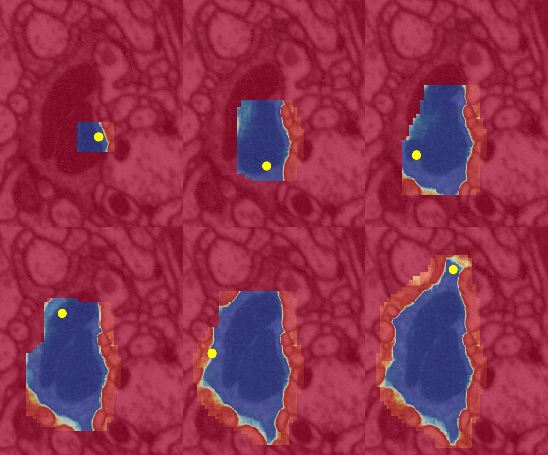
Tracing neurites in large-scale electron microscopy data is an example of an image segmentation problem. Traditional algorithms have divided the process into at least two steps: finding boundaries between neurites using an edge detector or a machine-learning classifier, and then grouping together image pixels that are not separated by a boundary using an algorithm like watershed or graph cut. In 2015, we began experimenting with an alternative approach based on recurrent neural networks that unifies these two steps. The algorithm is seeded at a specific pixel location and then iteratively “fills” a region using a recurrent convolutional neural network that predicts which pixels are part of the same object as the seed. Since 2015, we have been working to apply this new approach to large-scale connectomics datasets and rigorously quantify its accuracy.
A flood-filling network segmenting an object in 2d. The yellow dot is the center of the current area of focus; the algorithm expands the segmented region (blue) as it iteratively examines more of the overall image.
Measuring Accuracy via Expected Run Length
Working with our partners at the Max Planck Institute, we devised a metric we call “expected run length” (ERL) that measures the following: given a random point within a random neuron in a 3d image of a brain, how far can we trace the neuron before making some kind of mistake? This is an example of a mean-time-between-failure metric, except that in this case we measure the amount of space between failures rather than the amount of time. For engineers, the appeal of ERL is that it relates a linear, physical path length to the frequency of individual mistakes that are made by an algorithm, and that it can be computed in a straightforward way. For biologists, the appeal is that a particular numerical value of ERL can be related to biologically relevant quantities, such as the average path length of neurons in different parts of the nervous system.
Progress in expected run length (blue line) leading up to the results shared today in Nature Methods. The red line shows progress in the “merge rate,” which measures the frequency with which two separate neurites were erroneously traced as a single object; achieving a very low merge rate is important for enabling efficient strategies for manual identification and correction of the remaining errors in the reconstruction.
Songbird Connectomics
We used ERL to measure our progress on a ground-truth set of neurons within a 1-million cubic micron zebra finch song-bird brain imaged by our collaborators using serial block-face scanning electron microscopy and found that our approach performed much better than previous deep learning pipelines applied to the same dataset.
Our algorithm in action as it traces a single neurite in 3d in a songbird brain.
We segmented every neuron in a small portion of a zebra finch song-bird brain using the new flood-filling network approach, as depicted here:
Reconstruction of a portion of zebra finch brain. Colors denote distinct objects in the segmentation that was automatically generated using a flood-filling network. Gold spheres represent synaptic locations automatically identified using a previously published approach.
By combining these automated results with a small amount of additional human effort required to fix the remaining errors, our collaborators at the Max Planck Institute are now able to study the songbird connectome to derive new insights into how zebra finch birds sing their song and test theories related to how they learn their song.

Next Steps
We will continue to improve connectomics reconstruction technology, with the aim of fully automating synapse-resolution connectomics and contributing to ongoing connectomics projects at the Max Planck Institute and elsewhere. In order to help support the larger research community in developing connectomics techniques, we have also open-sourced the TensorFlow code for the flood-filling network approach, along with WebGL visualization software for 3d datasets that we developed to help us understand and improve our reconstruction results.

Acknowledgements
We would like to acknowledge core contributions from Tim Blakely, Peter Li, Larry Lindsey, Jeremy Maitin-Shepard, Art Pope and Mike Tyka (Google), as well as Joergen Kornfeld and Winfried Denk (Max Planck Institute).

Source: Google AI Blog


Accelerated Training and Inference with the Tensorflow Object Detection API


Last year we announced the TensorFlow Object Detection API, and since then we’ve released a number of new features, such as models learned via Neural Architecture Search, instance segmentation support and models trained on new datasets such as Open Images. We have been amazed at how it is being used – from finding scofflaws on the streets of NYC to diagnosing diseases on cassava plants in Tanzania.
Today, as part of Google’s commitment to democratizing computer vision, and using feedback from the research community on how to make this codebase even more useful, we’re excited to announce a number of additions to our API. Highlights of this release include:
  • Support for accelerated training of object detection models via Cloud TPUs
  • Improving the mobile deployment process by accelerating inference and making it easy to export a model to mobile with the TensorFlow Lite format
  • Several new model architecture definitions including:
Additionally, we are releasing pre-trained weights for each of the above models based on the COCO dataset.

Accelerated Training via Cloud TPUs
Users spend a great deal of time on optimizing hyperparameters and retraining object detection models, therefore having fast turnaround times on experiments is critical. The models released today belong to the single shot detector (SSD) class of architectures that are optimized for training on Cloud TPUs. For example, we can now train a ResNet-50 based RetinaNet model to achieve 35% mean Average Precision (mAP) on the COCO dataset in < 3.5 hrs.
Accelerated Inference via Quantization and TensorFlow Lite 
To better support low-latency requirements on mobile and embedded devices, the models we are providing are now natively compatible with TensorFlow Lite, which enables on-device machine learning inference with low latency and a small binary size. As part of this, we have implemented: (1) model quantization and (2) detection-specific operations natively in TensorFlow Lite. Our model quantization follows the strategy outlined in Jacob et al. (2018) and the whitepaper by Krishnamoorthi (2018) which applies quantization to both model weights and activations at training and inference time, yielding smaller models that run faster.
Quantized detection models are faster and smaller (e.g., a quantized 75% depth-reduced SSD Mobilenet model runs at >15 fps on a Pixel 2 CPU with a 4.2 Mb footprint) with minimal loss in detection accuracy compared to the full floating point model.
Try it Yourself with a New Tutorial!
To get started training your own model on Cloud TPUs, check out our new tutorial! This walkthrough will take you through the process of training a quantized pet face detector on Cloud TPU then exporting it to an Android phone for inference via TensorFlow Lite conversion.

We hope that these new additions will help make high-quality computer vision models accessible to anyone wishing to solve an object detection problem, and provide a more seamless user experience, from training a model with quantization to exporting to a TensorFlow Lite model ready for on-device deployment. We would like to thank everyone in the community who have contributed features and bug fixes. As always, contributions to the codebase are welcome, and please stay tuned for more updates!

Acknowledgements
This post reflects the work of the following group of core contributors: Derek Chow, Aakanksha Chowdhery, Jonathan Huang, Pengchong Jin, Zhichao Lu, Vivek Rathod, Ronny Votel and Xiangxin Zhu. We would also like to thank the following colleagues: Vasu Agrawal, Sourabh Bajaj, Chiachen Chou, Tom Jablin, Wenzhe Li, Tsung-Yi Lin, Hernan Moraldo, Kevin Murphy, Sara Robinson, Andrew Selle, Shashi Shekhar, Yash Sonthalia, Zak Stone, Pete Warden and Menglong Zhu.

Source: Google AI Blog


Automating Drug Discoveries Using Computer Vision


“Every time you miss a protein crystal, because they are so rare, you risk missing on an important biomedical discovery.”
- Patrick Charbonneau, Duke University Dept. of Chemistry and Lead Researcher, MARCO initiative.

Protein crystallization is a key step to biomedical research concerned with discovering the structure of complex biomolecules. Because that structure determines the molecule’s function, it helps scientists design new drugs that are specifically targeted to that function. However, protein crystals are rare and difficult to find. Hundreds of experiments are typically run for each protein, and while the setup and imaging are mostly automated, finding individual protein crystals remains largely performed through visual inspection and thus prone to human error. Critically, missing these structures can result in lost opportunity for important biomedical discoveries for advancing the state of medicine.

In collaboration with researchers from the MAchine Recognition of Crystallization Outcomes (MARCO) initiative, we have published “Classification of Crystallization Outcomes using Deep Convolutional Neural Networks” in PLOS One (ArXiv preprint), in which we discuss how we used some of the most recent architectures of deep convolutional networks and customized them to achieve an accuracy of more than 94% on the visual recognition task of identifying protein crystals. In order to spur further research in this area, we have made the data freely accessible, and open-sourced our model as part of the TensorFlow research model repository, and available to researchers as a Cloud ML Engine endpoint.
Image of protein crystal, courtesy of the MARCO repository (CC-BY-4.0 license)
The MARCO initiative is a joint project between several pharmaceutical companies and academic research centers to pool and host a large repository of curated crystallography images, and make them available to the community to help develop better image analysis tools. When a member of the initiative reached out to Google with a well-defined problem, and half a million labelled images, we embraced the challenge of trying to apply the recent advances in deep learning to the problem.

Due to the large variability between imaging technologies and data acquisition approaches, coming up with a single approach to the visual recognition problem may appear daunting. Crystals can be very small, which makes them rare structures in a large image containing otherwise undifferentiated visual clutter.
Samples from the MARCO repository, illustrating the degree of variability between data sources.
Fortunately, given sufficient training data, modern deep convolutional networks are well suited to handle extreme variability in visual appearance. We modified the basic Inception V3 model to handle larger images while still being able to be trained quickly. The model achieves a level of precision and recall that makes its use practical in automated assessment pipelines.

This work is a great example of the effectiveness of multi-institutional collaborations aimed at solving problems that require data in amounts and level of diversity that no single collaborator has access to. We invite researchers to take advantage of these resources that are the result of this work and share what they learn. This research was conducted as a personal 20% project by the author. To learn more about this work, please see our paper here and read the recent Duke Research Blog post.

Source: Google AI Blog


Google at ICML 2018


Machine learning is a key strategic focus at Google, with highly active groups pursuing research in virtually all aspects of the field, including deep learning and more classical algorithms, exploring theory as well as application. We utilize scalable tools and architectures to build machine learning systems that enable us to solve deep scientific and engineering challenges in areas of language, speech, translation, music, visual processing and more.

As a leader in machine learning research, Google is proud to be a Platinum Sponsor of the thirty-fifth International Conference on Machine Learning (ICML 2018), a premier annual event supported by the International Machine Learning Society taking place this week in Stockholm, Sweden. With over 130 Googlers attending the conference to present publications and host workshops, we look forward to our continued collaboration with the larger ML research community.

If you're attending ICML 2018, we hope you'll visit the Google booth and talk with our researchers to learn more about the exciting work, creativity and fun that goes into solving some of the field's most interesting challenges. Our researchers will also be available to talk about TensorFlow Hub, the latest work from the Magenta project, a Q&A session on the Google AI Residency program and much more. You can also learn more about our research being presented at ICML 2018 in the list below (Googlers highlighted in blue).

ICML 2018 Committees
Board Members include: Andrew McCallumCorinna CortesHugo LarochelleWilliam Cohen
Sponsorship Co-Chair: Ryan Adams

Accepted Publications
Predict and Constrain: Modeling Cardinality in Deep Structured Prediction
Nataly Brukhim, Amir Globerson

Quickshift++: Provably Good Initializations for Sample-Based Mean Shift
Heinrich Jiang, Jennifer Jang, Samory Kpotufe

Learning a Mixture of Two Multinomial Logits
Flavio Chierichetti, Ravi KumarAndrew Tomkins

Structured Evolution with Compact Architectures for Scalable Policy Optimization
Krzysztof Choromanski, Mark Rowland, Vikas Sindhwani, Richard E Turner, Adrian Weller

Fixing a Broken ELBO
Alexander Alemi, Ben Poole, Ian FischerJoshua DillonRif SaurousKevin Murphy

Hierarchical Long-term Video Prediction without Supervision
Nevan Wichers, Ruben Villegas, Dumitru ErhanHonglak Lee

Self-Consistent Trajectory Autoencoder: Hierarchical Reinforcement Learning with Trajectory Embeddings
John Co-Reyes, Yu Xuan Liu, Abhishek Gupta, Benjamin Eysenbach, Pieter Abbeel, Sergey Levine

Well Tempered Lasso
Yuanzhi Li, Yoram Singer

Programmatically Interpretable Reinforcement Learning
Abhinav Verma, Vijayaraghavan Murali, Rishabh Singh, Pushmeet Kohli, Swarat Chaudhuri

Dynamical Isometry and a Mean Field Theory of CNNs: How to Train 10,000-Layer Vanilla Convolutional Neural Networks
Lechao XiaoYasaman BahriJascha Sohl-DicksteinSamuel SchoenholzJeffrey Pennington

On the Optimization of Deep Networks: Implicit Acceleration by Overparameterization
Sanjeev Arora, Nadav Cohen, Elad Hazan

Scalable Deletion-Robust Submodular Maximization: Data Summarization with Privacy and Fairness Constraints
Ehsan Kazemi, Morteza Zadimoghaddam, Amin Karbasi

Data Summarization at Scale: A Two-Stage Submodular Approach
Marko Mitrovic, Ehsan Kazemi, Morteza Zadimoghaddam, Amin Karbasi

Machine Theory of Mind
Neil Rabinowitz, Frank Perbet, Francis Song, Chiyuan Zhang, S. M. Ali Eslami, Matthew Botvinick

Learning to Optimize Combinatorial Functions
Nir Rosenfeld, Eric Balkanski, Amir Globerson, Yaron Singer

Proportional Allocation: Simple, Distributed, and Diverse Matching with High Entropy
Shipra Agarwal, Morteza ZadimoghaddamVahab Mirrokni

Path Consistency Learning in Tsallis Entropy Regularized MDPs
Yinlam Chow, Ofir NachumMohammad Ghavamzadeh

Efficient Neural Architecture Search via Parameters Sharing
Hieu Pham, Melody Guan, Barret ZophQuoc LeJeff Dean

Adafactor: Adaptive Learning Rates with Sublinear Memory Cost
Noam Shazeer, Mitchell Stern

Learning Memory Access Patterns
Milad HashemiKevin SwerskyJamie Smith, Grant Ayers, Heiner Litz, Jichuan Chang, Christos Kozyrakis, Parthasarathy Ranganathan

SBEED: Convergent Reinforcement Learning with Nonlinear Function Approximation
Bo Dai, Albert Shaw, Lihong Li, Lin Xiao, Niao He, Zhen Liu, Jianshu Chen, Le Song

Scalable Bilinear Pi Learning Using State and Action Features
Yichen Chen, Lihong Li, Mengdi Wang

Distributed Asynchronous Optimization with Unbounded Delays: How Slow Can You Go?
Zhengyuan Zhou, Panayotis Mertikopoulos, Nicholas Bambos, Peter Glynn, Yinyu Ye, Li-Jia Li, Li Fei-Fei

Shampoo: Preconditioned Stochastic Tensor Optimization
Vineet Gupta, Tomer Koren, Yoram Singer

Parallel and Streaming Algorithms for K-Core Decomposition
Hossein Esfandiari, Silvio LattanziVahab Mirrokni

Can Deep Reinforcement Learning Solve Erdos-Selfridge-Spencer Games?
Maithra RaghuAlexander Irpan, Jacob Andreas, Bobby Kleinberg, Quoc Le, Jon Kleinberg

Is Generator Conditioning Causally Related to GAN Performance?
Augustus OdenaJacob BuckmanCatherine OlssonTom BrownChristopher OlahColin RaffelIan Goodfellow

The Mirage of Action-Dependent Baselines in Reinforcement Learning
George TuckerSurya Bhupatiraju, Shixiang Gu, Richard E Turner, Zoubin Ghahramani, Sergey Levine

MentorNet: Learning Data-Driven Curriculum for Very Deep Neural Networks on Corrupted Labels
Lu Jiang, Zhengyuan Zhou, Thomas Leung, Li-Jia LiLi Fei-Fei

Loss Decomposition for Fast Learning in Large Output Spaces
En-Hsu Yen, Satyen KaleFelix Xinnan YuDaniel Holtmann-RiceSanjiv Kumar, Pradeep Ravikumar

A Hierarchical Latent Vector Model for Learning Long-Term Structure in Music
Adam RobertsJesse EngelColin RaffelCurtis HawthorneDouglas Eck

Smoothed Action Value Functions for Learning Gaussian Policies
Ofir NachumMohammad NorouziGeorge TuckerDale Schuurmans

Fast Decoding in Sequence Models Using Discrete Latent Variables
Lukasz KaiserSamy BengioAurko RoyAshish VaswaniNiki ParmarJakob UszkoreitNoam Shazeer

Accelerating Greedy Coordinate Descent Methods
Haihao Lu, Robert Freund, Vahab Mirrokni

Approximate Leave-One-Out for Fast Parameter Tuning in High Dimensions
Shuaiwen Wang, Wenda Zhou, Haihao Lu, Arian Maleki, Vahab Mirrokni

Image Transformer
Niki Parmar, Ashish Vaswani, Jakob Uszkoreit, Lukasz Kaiser, Noam Shazeer, Alexander Ku, Dustin Tran

Towards End-to-End Prosody Transfer for Expressive Speech Synthesis with Tacotron
RJ Skerry-Ryan, Eric Battenberg, Ying Xiao, Yuxuan Wang, Daisy Stanton, Joel Shor, Ron Weiss, Robert Clark, Rif Saurous

Dynamical Isometry and a Mean Field Theory of RNNs: Gating Enables Signal Propagation in Recurrent Neural Networks
Minmin Chen, Jeffrey Pennington,, Samuel Schoenholz

Style Tokens: Unsupervised Style Modeling, Control and Transfer in End-to-End Speech Synthesis
Yuxuan Wang, Daisy Stanton, Yu Zhang, RJ Skerry-Ryan, Eric Battenberg, Joel ShorYing Xiao, Ye Jia, Fei Ren, Rif Saurous

Constrained Interacting Submodular Groupings
Andrew CotterMahdi Milani FardSeungil YouMaya Gupta, Jeff Bilmes

Reinforcing Adversarial Robustness using Model Confidence Induced by Adversarial Training
Xi Wu, Uyeong Jang, Jiefeng Chen, Lingjiao Chen, Somesh Jha

Interpretability Beyond Feature Attribution: Quantitative Testing with Concept Activation Vectors (TCAV)
Been Kim, Martin Wattenberg, Justin Gilmer, Carrie Cai, James Wexler, Fernanda Viégas, Rory Sayres

Online Learning with Abstention
Corinna CortesGiulia DeSalvoClaudio GentileMehryar Mohri, Scott Yang

Online Linear Quadratic Control
Alon CohenAvinatan HasidimTomer KorenNevena LazicYishay MansourKunal Talwar

Competitive Caching with Machine Learned Advice
Thodoris Lykouris, Sergei Vassilvitskii

Efficient Neural Audio Synthesis
Nal Kalchbrenner, Erich Elsen, Karen Simonyan, Seb Noury, Norman Casagrande, Edward Lockhart, Florian Stimberg, Aäron van den Oord, Sander Dieleman, Koray Kavukcuoglu

Gradient Descent with Identity Initialization Efficiently Learns Positive Definite Linear Transformations by Deep Residual Networks
Peter Bartlett, Dave Helmbold, Phil Long

Understanding and Simplifying One-Shot Architecture Search
Gabriel BenderPieter-Jan KindermansBarret ZophVijay VasudevanQuoc Le

Approximation Algorithms for Cascading Prediction Models
Matthew Streeter

Learning Longer-term Dependencies in RNNs with Auxiliary Losses
Trieu TrinhAndrew DaiThang LuongQuoc Le

Self-Imitation Learning
Junhyuk Oh, Yijie Guo, Satinder Singh, Honglak Lee

Adaptive Sampled Softmax with Kernel Based Sampling
Guy Blanc, Steffen Rendle

Workshops
2018 Workshop on Human Interpretability in Machine Learning (WHI)
Organizers: Been Kim, Kush Varshney, Adrian Weller
Invited Speakers include: Fernanda ViégasMartin Wattenberg

Exploration in Reinforcement Learning
Organizers: Ben EysenbachSurya BhupatirajuShane Gu, Junhyuk Oh, Vincent Vanhoucke, Oriol Vinyals, Doina Precup

Theoretical Foundations and Applications of Deep Generative Models
Invited speakers include: Honglak Lee

Source: Google AI Blog


Scalable Deep Reinforcement Learning for Robotic Manipulation


How can robots acquire skills that generalize effectively to diverse, real-world objects and situations? While designing robotic systems that effectively perform repetitive tasks in controlled environments, like building products on an assembly line, is fairly routine, designing robots that can observe their surroundings and decide the best course of action while reacting to unexpected outcomes is exceptionally difficult. However, there are two tools that can help robots acquire such skills from experience: deep learning, which is excellent at handling unstructured real-world scenarios, and reinforcement learning, which enables longer-term reasoning while exhibiting more complex and robust sequential decision making. Combining these two techniques has the potential to enable robots to learn continuously from their experience, allowing them to master basic sensorimotor skills using data rather than manual engineering.

Designing reinforcement learning algorithms for robot learning introduces its own set of challenges: real-world objects span a wide variety of visual and physical properties, subtle differences in contact forces can make predicting object motion difficult and objects of interest can be obstructed from view. Furthermore, robotic sensors are inherently noisy, adding to the complexity. All of these factors makes it incredibly difficult to learn a general solution, unless there is enough variety in the training data, which takes time to collect. This motivates exploring learning algorithms that can effectively reuse past experience, similar to our previous work on grasping which benefited from large datasets. However, this previous work could not reason about the long-term consequences of its actions, which is important for learning how to grasp. For example, if multiple objects are clumped together, pushing one of them apart (called “singulation”) will make the grasp easier, even if doing so does not directly result in a successful grasp.
Examples of singulation.

To be more efficient, we need to use off-policy reinforcement learning, which can learn from data that was collected hours, days, or weeks ago. To design such an off-policy reinforcement learning algorithm that can benefit from large amounts of diverse experience from past interactions, we combined large-scale distributed optimization with a new fitted deep Q-learning algorithm that we call QT-Opt. A preprint is available on arXiv.

QT-Opt is a distributed Q-learning algorithm that supports continuous action spaces, making it well-suited to robotics problems. To use QT-Opt, we first train a model entirely offline, using whatever data we’ve already collected. This doesn’t require running the real robot, making it easier to scale. We then deploy and finetune that model on the real robot, further training it on newly collected data. As we run QT-Opt, we accumulate more offline data, letting us train better models, which lets us collect better data, and so on.

To apply this approach to robotic grasping, we used 7 real-world robots, which ran for 800 total robot hours over the course of 4 months. To bootstrap collection, we started with a hand-designed policy that succeeded 15-30% of the time. Data collection switched to the learned model when it started performing better. The policy takes a camera image and returns how the arm and gripper should move. The offline data contained grasps on over 1000 different objects.
Some of the training objects used.
In the past, we’ve seen that sharing experience across robots can accelerate learning. We scaled this training and data gathering process to ten GPUs, seven robots, and many CPUs, allowing us to collect and process a large dataset of over 580,000 grasp attempts. At the end of this process, we successfully trained a grasping policy that runs on a real world robot and generalizes to a diverse set of challenging objects that were not seen at training time.
Seven robots collecting grasp data.
Quantitatively, the QT-Opt approach succeeded in 96% of the grasp attempts across 700 trial grasps on previously unseen objects. Compared to our previous supervised-learning based grasping approach, which had a 78% success rate, our method reduced the error rate by more than a factor of five.
The objects used at evaluation time. To make the task challenging, we aimed for a large variety of object sizes, textures, and shapes.

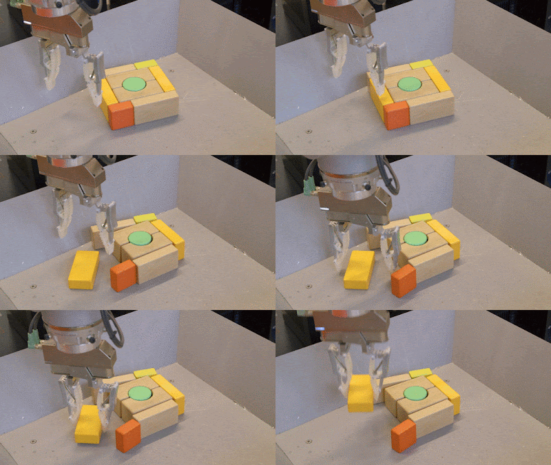
Notably, the policy exhibits a variety of closed-loop, reactive behaviors that are often not found in standard robotic grasping systems:
  • When presented with a set of interlocking blocks that cannot be picked up together, the policy separates one of the blocks from the rest before picking it up.
  • When presented with a difficult-to-grasp object, the policy figures out it should reposition the gripper and regrasp it until it has a firm hold.
  • When grasping in clutter, the policy probes different objects until the fingers hold one of them firmly, before lifting.
  • When we perturbed the robot by intentionally swatting the object out of the gripper -- something it had not seen during training -- it automatically repositioned the gripper for another attempt.
Crucially, none of these behaviors were engineered manually. They emerged automatically from self-supervised training with QT-Opt, because they improve the model’s long-term grasp success.
Examples of the learned behaviors. In the left GIF, the policy corrects for the moved ball. In the right GIF, the policy tries several grasps until it succeeds at picking up the tricky object.

Additionally, we’ve found that QT-Opt reaches this higher success rate using less training data, albeit with taking longer to converge. This is especially exciting for robotics, where the bottleneck is usually collecting real robot data, rather than training time. Combining this with other data efficiency techniques (such as our prior work on domain adaptation for grasping) could open several interesting avenues in robotics. We’re also interested in combining QT-Opt with recent work on learning how to self-calibrate, which could further improve the generality.

Overall, the QT-Opt algorithm is a general reinforcement learning approach that’s giving us good results on real world robots. Besides the reward definition, nothing about QT-Opt is specific to robot grasping. We see this as a strong step towards more general robot learning algorithms, and are excited to see what other robotics tasks we can apply it to. You can learn more about this work in the short video below.
Acknowledgements
This research was conducted by Dmitry Kalashnikov, Alex Irpan, Peter Pastor, Julian Ibarz, Alexander Herzog, Eric Jang, Deirdre Quillen, Ethan Holly, Mrinal Kalakrishnan, Vincent Vanhoucke, and Sergey Levine. We’d also like to give special thanks to Iñaki Gonzalo and John-Michael Burke for overseeing the robot operations, Chelsea Finn, Timothy Lillicrap, and Arun Nair for valuable discussions, and other people at Google and X who’ve contributed their expertise and time towards this research. A preprint is available on arXiv.

Source: Google AI Blog