Tag Archives: Machine Perception

Announcing the ICDAR 2023 Competition on Hierarchical Text Detection and Recognition

The last few decades have witnessed the rapid development of Optical Character Recognition (OCR) technology, which has evolved from an academic benchmark task used in early breakthroughs of deep learning research to tangible products available in consumer devices and to third party developers for daily use. These OCR products digitize and democratize the valuable information that is stored in paper or image-based sources (e.g., books, magazines, newspapers, forms, street signs, restaurant menus) so that they can be indexed, searched, translated, and further processed by state-of-the-art natural language processing techniques.

Research in scene text detection and recognition (or scene text spotting) has been the major driver of this rapid development through adapting OCR to natural images that have more complex backgrounds than document images. These research efforts, however, focus on the detection and recognition of each individual word in images, without understanding how these words compose sentences and articles.

Layout analysis is another relevant line of research that takes a document image and extracts its structure, i.e., title, paragraphs, headings, figures, tables and captions. These layout analysis efforts are parallel to OCR and have been largely developed as independent techniques that are typically evaluated only on document images. As such, the synergy between OCR and layout analysis remains largely under-explored. We believe that OCR and layout analysis are mutually complementary tasks that enable machine learning to interpret text in images and, when combined, could improve the accuracy and efficiency of both tasks.

With this in mind, we announce the Competition on Hierarchical Text Detection and Recognition (the HierText Challenge), hosted as part of the 17th annual International Conference on Document Analysis and Recognition (ICDAR 2023). The competition is hosted on the Robust Reading Competition website, and represents the first major effort to unify OCR and layout analysis. In this competition, we invite researchers from around the world to build systems that can produce hierarchical annotations of text in images using words clustered into lines and paragraphs. We hope this competition will have a significant and long-term impact on image-based text understanding with the goal to consolidate the research efforts across OCR and layout analysis, and create new signals for downstream information processing tasks.

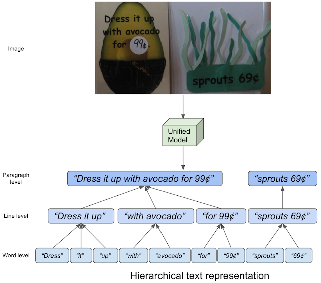
The concept of hierarchical text representation.


Constructing a hierarchical text dataset

In this competition, we use the HierText dataset that we published at CVPR 2022 with our paper "Towards End-to-End Unified Scene Text Detection and Layout Analysis". It’s the first real-image dataset that provides hierarchical annotations of text, containing word, line, and paragraph level annotations. Here, "words" are defined as sequences of textual characters not interrupted by spaces. "Lines" are then interpreted as "space"-separated clusters of "words" that are logically connected in one direction, and aligned in spatial proximity. Finally, "paragraphs" are composed of "lines" that share the same semantic topic and are geometrically coherent.

To build this dataset, we first annotated images from the Open Images dataset using the Google Cloud Platform (GCP) Text Detection API. We filtered through these annotated images, keeping only images rich in text content and layout structure. Then, we worked with our third-party partners to manually correct all transcriptions and to label words, lines and paragraph composition. As a result, we obtained 11,639 transcribed images, split into three subsets: (1) a train set with 8,281 images, (2) a validation set with 1,724 images, and (3) a test set with 1,634 images. As detailed in the paper, we also checked the overlap between our dataset, TextOCR, and Intel OCR (both of which also extracted annotated images from Open Images), making sure that the test images in the HierText dataset were not also included in the TextOCR or Intel OCR training and validation splits and vice versa. Below, we visualize examples using the HierText dataset and demonstrate the concept of hierarchical text by shading each text entity with different colors. We can see that HierText has a diversity of image domain, text layout, and high text density.

Samples from the HierText dataset. Left: Illustration of each word entity. Middle: Illustration of line clustering. Right: Illustration paragraph clustering.


Dataset with highest density of text

In addition to the novel hierarchical representation, HierText represents a new domain of text images. We note that HierText is currently the most dense publicly available OCR dataset. Below we summarize the characteristics of HierText in comparison with other OCR datasets. HierText identifies 103.8 words per image on average, which is more than 3x the density of TextOCR and 25x more dense than ICDAR-2015. This high density poses unique challenges for detection and recognition, and as a consequence HierText is used as one of the primary datasets for OCR research at Google.


Dataset       Training split       Validation split       Testing split       Words per image      
ICDAR-2015       1,000       0       500       4.4      
TextOCR       21,778       3,124       3,232       32.1      
Intel OCR       19,1059       16,731       0       10.0      
HierText       8,281       1,724       1,634       103.8

Comparing several OCR datasets to the HierText dataset.


Spatial distribution

We also find that text in the HierText dataset has a much more even spatial distribution than other OCR datasets, including TextOCR, Intel OCR, IC19 MLT, COCO-Text and IC19 LSVT. These previous datasets tend to have well-composed images, where text is placed in the middle of the images, and are thus easier to identify. On the contrary, text entities in HierText are broadly distributed across the images. It's proof that our images are from more diverse domains. This characteristic makes HierText uniquely challenging among public OCR datasets.

Spatial distribution of text instances in different datasets.


The HierText challenge

The HierText Challenge represents a novel task and with unique challenges for OCR models. We invite researchers to participate in this challenge and join us in ICDAR 2023 this year in San Jose, CA. We hope this competition will spark research community interest in OCR models with rich information representations that are useful for novel down-stream tasks.


Acknowledgements

The core contributors to this project are Shangbang Long, Siyang Qin, Dmitry Panteleev, Alessandro Bissacco, Yasuhisa Fujii and Michalis Raptis. Ashok Popat and Jake Walker provided valuable advice. We also thank Dimosthenis Karatzas and Sergi Robles from Autonomous University of Barcelona for helping us set up the competition website.

Source: Google AI Blog


Infinite Nature: Generating 3D Flythroughs from Still Photos

We live in a world of great natural beauty — of majestic mountains, dramatic seascapes, and serene forests. Imagine seeing this beauty as a bird does, flying past richly detailed, three-dimensional landscapes. Can computers learn to synthesize this kind of visual experience? Such a capability would allow for new kinds of content for games and virtual reality experiences: for instance, relaxing within an immersive flythrough of an infinite nature scene. But existing methods that synthesize new views from images tend to allow for only limited camera motion.

In a research effort we call Infinite Nature, we show that computers can learn to generate such rich 3D experiences simply by viewing nature videos and photographs. Our latest work on this theme, InfiniteNature-Zero (presented at ECCV 2022) can produce high-resolution, high-quality flythroughs starting from a single seed image, using a system trained only on still photographs, a breakthrough capability not seen before. We call the underlying research problem perpetual view generation: given a single input view of a scene, how can we synthesize a photorealistic set of output views corresponding to an arbitrarily long, user-controlled 3D path through that scene? Perpetual view generation is very challenging because the system must generate new content on the other side of large landmarks (e.g., mountains), and render that new content with high realism and in high resolution.


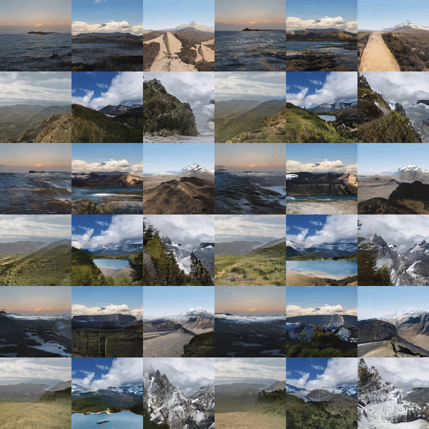
Example flythrough generated with InfiniteNature-Zero. It takes a single input image of a natural scene and synthesizes a long camera path flying into that scene, generating new scene content as it goes.

Background: Learning 3D Flythroughs from Videos

To establish the basics of how such a system could work, we’ll describe our first version, “Infinite Nature: Perpetual View Generation of Natural Scenes from a Single Image” (presented at ICCV 2021). In that work we explored a “learn from video” approach, where we collected a set of online videos captured from drones flying along coastlines, with the idea that we could learn to synthesize new flythroughs that resemble these real videos. This set of online videos is called the Aerial Coastline Imagery Dataset (ACID). In order to learn how to synthesize scenes that respond dynamically to any desired 3D camera path, however, we couldn’t simply treat these videos as raw collections of pixels; we also had to compute their underlying 3D geometry, including the camera position at each frame.

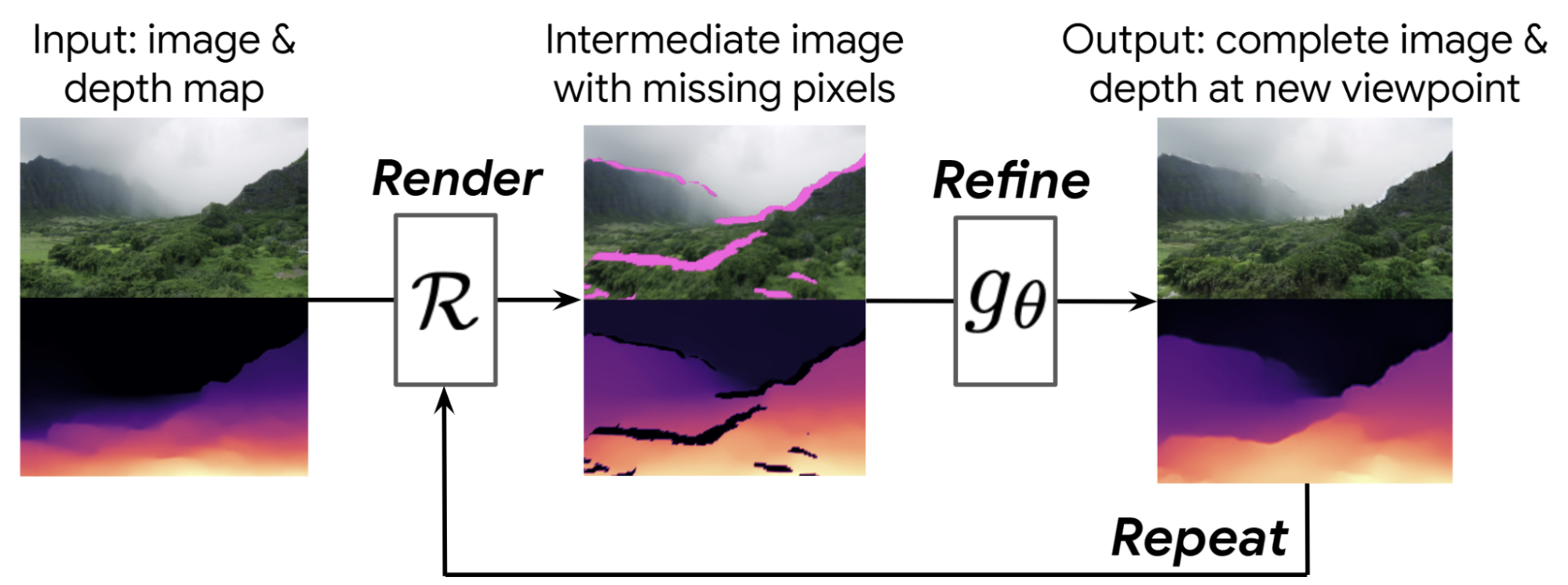
The basic idea is that we learn to generate flythroughs step-by-step. Given a starting view, like the first image in the figure below, we first compute a depth map using single-image depth prediction methods. We then use that depth map to render the image forward to a new camera viewpoint, shown in the middle, resulting in a new image and depth map from that new viewpoint.

However, this intermediate image has some problems — it has holes where we can see behind objects into regions that weren’t visible in the starting image. It is also blurry, because we are now closer to objects, but are stretching the pixels from the previous frame to render these now-larger objects.

To handle these problems, we learn a neural image refinement network that takes this low-quality intermediate image and outputs a complete, high-quality image and corresponding depth map. These steps can then be repeated, with this synthesized image as the new starting point. Because we refine both the image and the depth map, this process can be iterated as many times as desired — the system automatically learns to generate new scenery, like mountains, islands, and oceans, as the camera moves further into the scene.

Our Infinite Nature methods take an input view and its corresponding depth map (left). Using this depth map, the system renders the input image to a new desired viewpoint (center). This intermediate image has problems, such as missing pixels revealed behind foreground content (shown in magenta). We learn a deep network that refines this image to produce a new high-quality image (right). This process can be repeated to produce a long trajectory of views. We thus call this approach “render-refine-repeat”.

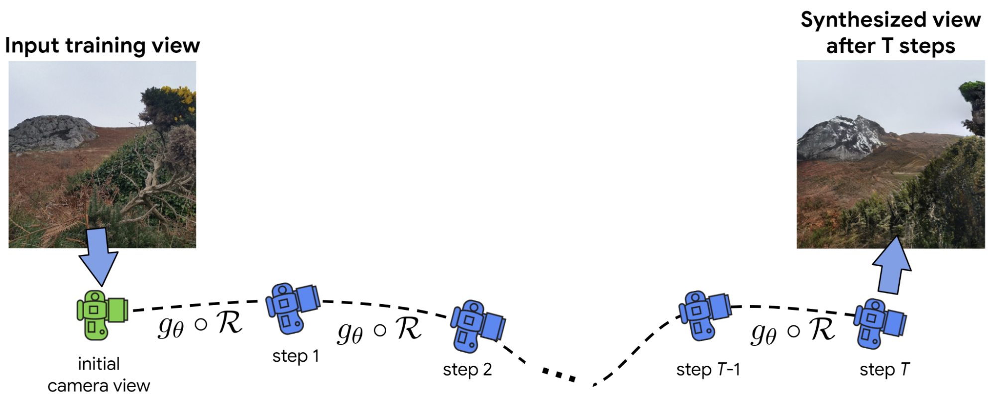
We train this render-refine-repeat synthesis approach using the ACID dataset. In particular, we sample a video from the dataset and then a frame from that video. We then use this method to render several new views moving into the scene along the same camera trajectory as the ground truth video, as shown in the figure below, and compare these rendered frames to the corresponding ground truth video frames to derive a training signal. We also include an adversarial setup that tries to distinguish synthesized frames from real images, encouraging the generated imagery to appear more realistic.

Infinite Nature can synthesize views corresponding to any camera trajectory. During training, we run our system for T steps to generate T views along a camera trajectory calculated from a training video sequence, then compare the resulting synthesized views to the ground truth ones. In the figure, each camera viewpoint is generated from the previous one by performing a warp operation R, followed by the neural refinement operation gθ.

The resulting system can generate compelling flythroughs, as featured on the project webpage, along with a “flight simulator” Colab demo. Unlike prior methods on video synthesis, this method allows the user to interactively control the camera and can generate much longer camera paths.


InfiniteNature-Zero: Learning Flythroughs from Still Photos

One problem with this first approach is that video is difficult to work with as training data. High-quality video with the right kind of camera motion is challenging to find, and the aesthetic quality of an individual video frame generally cannot compare to that of an intentionally captured nature photograph. Therefore, in “InfiniteNature-Zero: Learning Perpetual View Generation of Natural Scenes from Single Images”, we build on the render-refine-repeat strategy above, but devise a way to learn perpetual view synthesis from collections of still photos — no videos needed. We call this method InfiniteNature-Zero because it learns from “zero” videos. At first, this might seem like an impossible task — how can we train a model to generate video flythroughs of scenes when all it’s ever seen are isolated photos?

To solve this problem, we had the key insight that if we take an image and render a camera path that forms a cycle — that is, where the path loops back such that the last image is from the same viewpoint as the first — then we know that the last synthesized image along this path should be the same as the input image. Such cycle consistency provides a training constraint that helps the model learn to fill in missing regions and increase image resolution during each step of view generation.

However, training with these camera cycles is insufficient for generating long and stable view sequences, so as in our original work, we include an adversarial strategy that considers long, non-cyclic camera paths, like the one shown in the figure above. In particular, if we render T frames from a starting frame, we optimize our render-refine-repeat model such that a discriminator network can’t tell which was the starting frame and which was the final synthesized frame. Finally, we add a component trained to generate high-quality sky regions to increase the perceived realism of the results.

With these insights, we trained InfiniteNature-Zero on collections of landscape photos, which are available in large quantities online. Several resulting videos are shown below — these demonstrate beautiful, diverse natural scenery that can be explored along arbitrarily long camera paths. Compared to our prior work — and to prior video synthesis methods — these results exhibit significant improvements in quality and diversity of content (details available in the paper).


Several nature flythroughs generated by InfiniteNature-Zero from single starting photos.

Conclusion

There are a number of exciting future directions for this work. For instance, our methods currently synthesize scene content based only on the previous frame and its depth map; there is no persistent underlying 3D representation. Our work points towards future algorithms that can generate complete, photorealistic, and consistent 3D worlds.


Acknowledgements

Infinite Nature and InfiniteNature-Zero are the result of a collaboration between researchers at Google Research, UC Berkeley, and Cornell University. The key contributors to the work represented in this post include Angjoo Kanazawa, Andrew Liu, Richard Tucker, Zhengqi Li, Noah Snavely, Qianqian Wang, Varun Jampani, and Ameesh Makadia.

Source: Google AI Blog


Open Images V7 — Now Featuring Point Labels

Open Images is a computer vision dataset covering ~9 million images with labels spanning thousands of object categories. Researchers around the world use Open Images to train and evaluate computer vision models. Since the initial release of Open Images in 2016, which included image-level labels covering 6k categories, we have provided multiple updates to enrich annotations and expand the potential use cases of the dataset. Through several releases, we have added image-level labels for over 20k categories on all images and bounding box annotations, visual relations, instance segmentations, and localized narratives (synchronized voice, mouse trace, and text caption) on a subset of 1.9M images.

Today, we are happy to announce the release of Open Images V7, which expands the Open Images dataset even further with a new annotation type called point-level labels and includes a new all-in-one visualization tool that allows a better exploration of the rich data available.


Point Labels

The main strategy used to collect the new point-level label annotations leveraged suggestions from a machine learning (ML) model and human verification. First, the ML model selected points of interest and asked a yes or no question, e.g., “is this point on a pumpkin?”. Then, human annotators spent an average of 1.1 seconds answering the yes or no questions. We aggregated the answers from different annotators over the same question and assigned a final “yes”, “no”, or “unsure” label to each annotated point.

Illustration of the annotations interface.
(Image by Lenore Edman, under CC BY 2.0 license)

For each annotated image, we provide a collection of points, each with a “yes” or “no” label for a given class. These points provide sparse information that can be used for the semantic segmentation task. We collected a total of 38.6M new point annotations (12.4M with “yes” labels) that cover 5.8 thousand classes and 1.4M images.

By focusing on point labels, we expanded the number of images annotated and categories covered. We also concentrated the efforts of our annotators on efficiently collecting useful information. Compared to our instance segmentation, the new points include 16x more classes and cover more images. The new points also cover 9x more classes than our box annotations. Compared to existing segmentation datasets, like PASCAL VOC, COCO, Cityscapes, LVIS, or ADE20K, our annotations cover more classes and more images than previous work. The new point label annotations are the first type of annotation in Open Images that provides localization information for both things (countable objects, like cars, cats, and catamarans), and stuff categories (uncountable objects like grass, granite, and gravel). Overall, the newly collected data is roughly equivalent to two years of human annotation effort.

Our initial experiments show that this type of sparse data is suitable for both training and evaluating segmentation models. Training a model directly on sparse data allows us to reach comparable quality to training on dense annotations. Similarly, we show that one can directly compute the traditional semantic segmentation intersection-over-union (IoU) metric over sparse data. The ranking across different methods is preserved, and the sparse IoU values are an accurate estimate of its dense version. See our paper for more details.

Below, we show four example images with their point-level labels, illustrating the rich and diverse information these annotations provide. Circles ⭘ are “yes” labels, and squares are “no” labels.

Four example images with point-level labels.
Images by Richie Diesterheft, John AM Nueva, Sarah Ackerman, and C Thomas, all under CC BY 2.0 license.

New Visualizers

In addition to the new data release, we also expanded the available visualizations of the Open Images annotations. The Open Images website now includes dedicated visualizers to explore the localized narratives annotations, the new point-level annotations, and a new all-in-one view. This new all-in-one view is available for the subset of 1.9M densely annotated images and allows one to explore the rich annotations that Open Images has accumulated over seven releases. On average these images have annotations for 6.7 image-labels (classes), 8.3 boxes, 1.7 relations, 1.5 masks, 0.4 localized narratives and 34.8 point-labels per image.

Below, we show two example images with various annotations in the all-in-one visualizer. The figures show the image-level labels, bounding boxes, box relations, instance masks, localized narrative mouse trace and caption, and point-level labels. The + classes have positive annotations (of any kind), while classes have only negative annotations (image-level or point-level).

Two example images with various annotations in the all-in-one visualizer.
Images by Jason Paris, and Rubén Vique, all under CC BY 2.0 license.

Conclusion

We hope that this new data release will enable computer vision research to cover ever more diverse and challenging scenarios. As the quality of automated semantic segmentation models improves over common classes, we want to move towards the long tail of visual concepts, and sparse point annotations are a step in that direction. More and more works are exploring how to use such sparse annotations (e.g., as supervision for instance segmentation or semantic segmentation), and Open Images V7 contributes to this research direction. We are looking forward to seeing what you will build next.


Acknowledgements

Thanks to Vittorio Ferrari, Jordi Pont-Tuset, Alina Kuznetsova, Ashlesha Sadras, and the annotators team for their support creating this new data release.

Source: Google AI Blog


Learning to Walk in the Wild from Terrain Semantics

An important promise for quadrupedal robots is their potential to operate in complex outdoor environments that are difficult or inaccessible for humans. Whether it’s to find natural resources deep in the mountains, or to search for life signals in heavily-damaged earthquake sites, a robust and versatile quadrupedal robot could be very helpful. To achieve that, a robot needs to perceive the environment, understand its locomotion challenges, and adapt its locomotion skill accordingly. While recent advances in perceptive locomotion have greatly enhanced the capability of quadrupedal robots, most works focus on indoor or urban environments, thus they cannot effectively handle the complexity of off-road terrains. In these environments, the robot needs to understand not only the terrain shape (e.g., slope angle, smoothness), but also its contact properties (e.g., friction, restitution, deformability), which are important for a robot to decide its locomotion skills. As existing perceptive locomotion systems mostly focus on the use of depth cameras or LiDARs, it can be difficult for these systems to estimate such terrain properties accurately.

In “Learning Semantics-Aware Locomotion Skills from Human Demonstrations”, we design a hierarchical learning framework to improve a robot’s ability to traverse complex, off-road environments. Unlike previous approaches that focus on environment geometry, such as terrain shape and obstacle locations, we focus on environment semantics, such as terrain type (grass, mud, etc.) and contact properties, which provide a complementary set of information useful for off-road environments. As the robot walks, the framework decides the locomotion skill, including the speed and gait (i.e., shape and timing of the legs’ movement) of the robot based on the perceived semantics, which allows the robot to walk robustly on a variety of off-road terrains, including rocks, pebbles, deep grass, mud, and more.

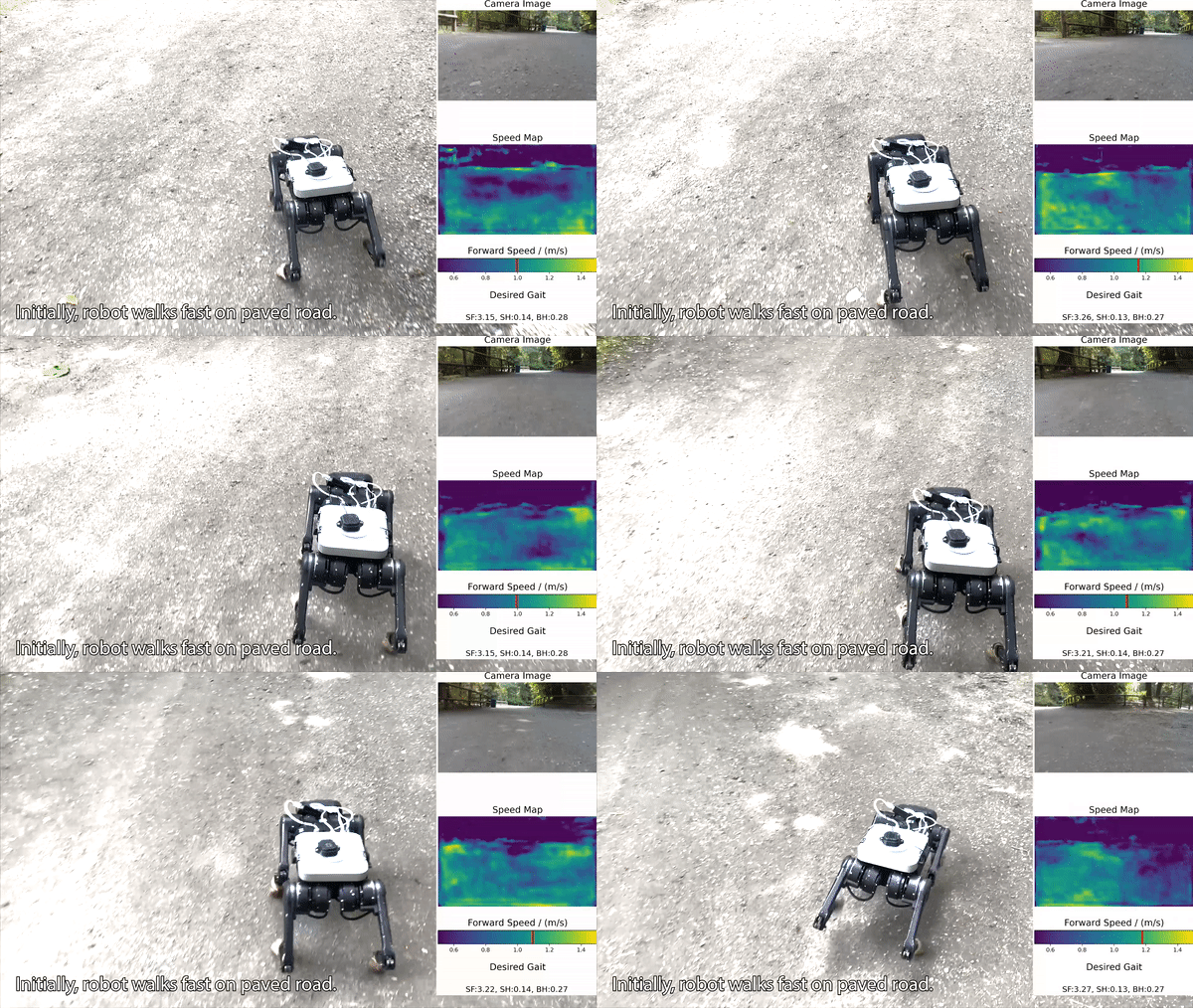
Our framework selects skills (gait and speed) of the robot from the camera RGB image. We first compute the speed from terrain semantics, and then select a gait based on the speed.

Overview
The hierarchical framework consists of a high-level skill policy and a low level motor controller. The skill policy selects a locomotion skill based on camera images, and the motor controller converts the selected skill into motor commands. The high-level skill policy is further decomposed into a learned speed policy and a heuristic-based gait selector. To decide a skill, the speed policy first computes the desired forward speed, based on the semantic information from the onboard RGB camera. For energy efficiency and robustness, quadrupedal robots usually select a different gait for each speed, so we designed the gait selector to compute a desired gait based on the forward speed. Lastly, a low-level convex model-predictive controller (MPC) converts the desired locomotion skill into motor torque commands, and executes them on the real hardware. We train the speed policy directly in the real world using imitation learning because it requires fewer training data compared to standard reinforcement learning algorithms.

The framework consists of a high-level skill policy and a low-level motor controller.

Learning Speed Command from Human Demonstrations
As the central component in our pipeline, the speed policy outputs the desired forward speed of the robot based on the RGB image from the onboard camera. Although many robot learning tasks can leverage simulation as a source of lower-cost data collection, we train the speed policy in the real world because accurate simulation of complex and diverse off-road environments is not yet available. As policy learning in the real world is time-consuming and potentially unsafe, we make two key design choices to improve the data efficiency and safety of our system.

The first is learning from human demonstrations. Standard reinforcement learning algorithms typically learn by exploration, where the agent attempts different actions in an environment and builds preferences based on the rewards received. However, such explorations can be potentially unsafe, especially in off-road environments, since any robot failures can damage both the robot hardware and the surrounding environment. To ensure safety, we train the speed policy using imitation learning from human demonstrations. We first ask a human operator to teleoperate the robot on a variety of off-road terrains, where the operator controls the speed and heading of the robot using a remote joystick. Next, we collect the training data by storing (image, forward_speed) pairs. We then train the speed policy using standard supervised learning to predict the human operator’s speed command. As it turns out, the human demonstration is both safe and high-quality, and allows the robot to learn a proper speed choice for different terrains.

The second key design choice is the training method. Deep neural networks, especially those involving high-dimensional visual inputs, typically require lots of data to train. To reduce the amount of real-world training data required, we first pre-train a semantic segmentation model on RUGD (an off-road driving dataset where the images look similar to those captured by the robot’s onboard camera), where the model predicts the semantic class (grass, mud, etc.) for every pixel in the camera image. We then extract a semantic embedding from the model’s intermediate layers and use that as the feature for on-robot training. With the pre-trained semantic embedding, we can train the speed policy effectively using less than 30 minutes of real-world data, which greatly reduces the amount of effort required.

We pre-train a semantic segmentation model and extract a semantic embedding to be fine-tuned on robot data.

Gait Selection and Motor Control
The next component in the pipeline, the gait selector, computes the appropriate gait based on the speed command from the speed policy. The gait of a robot, including its stepping frequency, swing height, and base height, can greatly affect the robot’s ability to traverse different terrains.

Scientific studies have shown that animals switch between different gaits at different speeds, and this result is further validated in quadrupedal robots, so we designed the gait selector to compute a robust gait for each speed. Compared to using a fixed gait across all speeds, we find that the gait selector further enhances the robot’s navigation performance on off-road terrains (more details in the paper).

The last component of the pipeline is a motor controller, which converts the speed and gait commands into motor torques. Similar to previous work, we use separate control strategies for swing and stance legs. By separating the task of skill learning and motor control, the skill policy only needs to output the desired speed, and does not need to learn low-level locomotion controls, which greatly simplifies the learning process.

Experiment Results
We implemented our framework on an A1 quadrupedal robot and tested it on an outdoor trail with multiple terrain types, including grass, gravel, and asphalt, which pose varying degrees of difficulty for the robot. For example, while the robot needs to walk slowly with high foot swings in deep grass to prevent its foot from getting stuck, on asphalt it can walk much faster with lower foot swings for better energy efficiency. Our framework captures such differences and selects an appropriate skill for each terrain type: slow speed (0.5m/s) on deep grass, medium speed (1m/s) on gravel, and high speed (1.4m/s) on asphalt. It completes the 460m-long trail in 9.6 minutes with an average speed of 0.8m/s (i.e., that’s 1.8 miles or 2.9 kilometers per hour). In contrast, non-adaptive policies either cannot complete the trail safely or walk significantly slower (0.5m/s), illustrating the importance of adapting locomotion skills based on the perceived environments.

The framework selects different speeds based on conditions of the trail.

To test generalizability, we also deployed the robot to a number of trails that are not seen during training. The robot traverses through all of them without failure, and adjusts its locomotion skills based on terrain semantics. In general, the skill policy selects a faster skill on rigid and flat terrains and a slower speed on deformable or uneven terrain. At the time of writing, the robot has traversed over 6km of outdoor trails without failure.

With the framework, the robot walks safely on a variety of outdoor terrains not seen during training.

Conclusion
In this work, we present a hierarchical framework to learn semantic-aware locomotion skills for off-road locomotion. Using less than 30 minutes of human demonstration data, the framework learns to adjust the speed and gait of the robot based on the perceived semantics of the environment. The robot can walk safely and efficiently on a wide variety of off-road terrains. One limitation of our framework is that it only adjusts locomotion skills for standard walking and does not support more agile behaviors such as jumping, which can be essential for traversing more difficult terrains with gaps or hurdles. Another limitation is that our framework currently requires manual steering commands to follow a desired path and reach the goal. In future work, we plan to look into a deeper integration of high-level skill policy with the low-level controller for more agile behaviors, and incorporate navigation and path planning into the framework so that the robot can operate fully autonomously in challenging off-road environments.

Acknowledgements
We would like to thank our paper co-authors: Xiangyun Meng, Wenhao Yu, Tingnan Zhang, Jie Tan, and Byron Boots. We would also like to thank the team members of Robotics at Google for discussions and feedback.

Source: Google AI Blog


High-Definition Segmentation in Google Meet

In recent years video conferencing has played an increasingly important role in both work and personal communication for many users. Over the past two years, we have enhanced this experience in Google Meet by introducing privacy-preserving machine learning (ML) powered background features, also known as “virtual green screen”, which allows users to blur their backgrounds or replace them with other images. What is unique about this solution is that it runs directly in the browser without the need to install additional software.

So far, these ML-powered features have relied on CPU inference made possible by leveraging neural network sparsity, a common solution that works across devices, from entry level computers to high-end workstations. This enables our features to reach the widest audience. However, mid-tier and high-end devices often have powerful GPUs that remain untapped for ML inference, and existing functionality allows web browsers to access GPUs via shaders (WebGL).

With the latest update to Google Meet, we are now harnessing the power of GPUs to significantly improve the fidelity and performance of these background effects. As we detail in “Efficient Heterogeneous Video Segmentation at the Edge”, these advances are powered by two major components: 1) a novel real-time video segmentation model and 2) a new, highly efficient approach for in-browser ML acceleration using WebGL. We leverage this capability to develop fast ML inference via fragment shaders. This combination results in substantial gains in accuracy and latency, leading to crisper foreground boundaries.

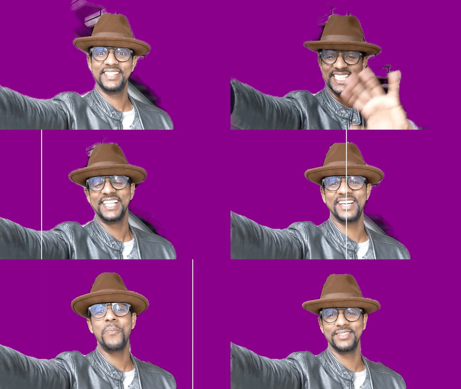
CPU segmentation vs. HD segmentation in Meet.

Moving Towards Higher Quality Video Segmentation Models
To predict finer details, our new segmentation model now operates on high definition (HD) input images, rather than lower-resolution images, effectively doubling the resolution over the previous model. To accommodate this, the model must be of higher capacity to extract features with sufficient detail. Roughly speaking, doubling the input resolution quadruples the computation cost during inference.

Inference of high-resolution models using the CPU is not feasible for many devices. The CPU may have a few high-performance cores that enable it to execute arbitrary complex code efficiently, but it is limited in its ability for the parallel computation required for HD segmentation. In contrast, GPUs have many, relatively low-performance cores coupled with a wide memory interface, making them uniquely suitable for high-resolution convolutional models. Therefore, for mid-tier and high-end devices, we adopt a significantly faster pure GPU pipeline, which is integrated using WebGL.

This change inspired us to revisit some of the prior design decisions for the model architecture.

  • Backbone: We compared several widely-used backbones for on-device networks and found EfficientNet-Lite to be a better fit for the GPU because it removes the squeeze-and-excitation block, a component that is inefficient on WebGL (more below).
  • Decoder: We switched to a multi-layer perceptron (MLP) decoder consisting of 1x1 convolutions instead of using simple bilinear upsampling or the more expensive squeeze-and-excitation blocks. MLP has been successfully adopted in other segmentation architectures, like DeepLab and PointRend, and is efficient to compute on both CPU and GPU.
  • Model size: With our new WebGL inference and the GPU-friendly model architecture, we were able to afford a larger model without sacrificing the real-time frame rate necessary for smooth video segmentation. We explored the width and the depth parameters using a neural architecture search.
HD segmentation model architecture.

In aggregate, these changes substantially improve the mean Intersection over Union (IoU) metric by 3%, resulting in less uncertainty and crisper boundaries around hair and fingers.

We have also released the accompanying model card for this segmentation model, which details our fairness evaluations. Our analysis shows that the model is consistent in its performance across the various regions, skin-tones, and genders, with only small deviations in IoU metrics.

Model     Resolution     Inference     IoU     Latency (ms)
CPU segmenter     256×144     Wasm SIMD     94.0%     8.7
GPU segmenter     512×288     WebGL     96.9%     4.3
Comparison of the previous segmentation model vs. the new HD segmentation model on a Macbook Pro (2018).

Accelerating Web ML with WebGL
One common challenge for web-based inference is that web technologies can incur a performance penalty when compared to apps running natively on-device. For GPUs, this penalty is substantial, only achieving around 25% of native OpenGL performance. This is because WebGL, the current GPU standard for Web-based inference, was primarily designed for image rendering, not arbitrary ML workloads. In particular, WebGL does not include compute shaders, which allow for general purpose computation and enable ML workloads in mobile and native apps.

To overcome this challenge, we accelerated low-level neural network kernels with fragment shaders that typically compute the output properties of a pixel like color and depth, and then applied novel optimizations inspired by the graphics community. As ML workloads on GPUs are often bound by memory bandwidth rather than compute, we focused on rendering techniques that would improve the memory access, such as Multiple Render Targets (MRT).

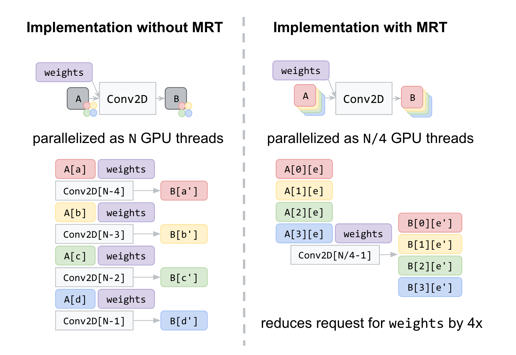
MRT is a feature in modern GPUs that allows rendering images to multiple output textures (OpenGL objects that represent images) at once. While MRT was originally designed to support advanced graphics rendering such as deferred shading, we found that we could leverage this feature to drastically reduce the memory bandwidth usage of our fragment shader implementations for critical operations, like convolutions and fully connected layers. We do so by treating intermediate tensors as multiple OpenGL textures.

In the figure below, we show an example of intermediate tensors having four underlying GL textures each. With MRT, the number of GPU threads, and thus effectively the number of memory requests for weights, is reduced by a factor of four and saves memory bandwidth usage. Although this introduces considerable complexities in the code, it helps us reach over 90% of native OpenGL performance, closing the gap with native applications.

Left: A classic implementation of Conv2D with 1-to-1 correspondence of tensor and an OpenGL texture. Red, yellow, green, and blue boxes denote different locations in a single texture each for intermediate tensor A and B. Right: Our implementation of Conv2D with MRT where intermediate tensors A and B are realized with a set of 4 GL textures each, depicted as red, yellow, green, and blue boxes. Note that this reduces the request count for weights by 4x.

Conclusion
We have made rapid strides in improving the quality of real-time segmentation models by leveraging the GPU on mid-tier and high-end devices for use with Google Meet. We look forward to the possibilities that will be enabled by upcoming technologies like WebGPU, which bring compute shaders to the web. Beyond GPU inference, we're also working on improving the segmentation quality for lower powered devices with quantized inference via XNNPACK WebAssembly.

Acknowledgements
Special thanks to those on the Meet team and others who worked on this project, in particular Sebastian Jansson, Sami Kalliomäki, Rikard Lundmark, Stephan Reiter, Fabian Bergmark, Ben Wagner, Stefan Holmer, Dan Gunnarsson, Stéphane Hulaud, and to all our team members who made this possible: Siargey Pisarchyk, Raman Sarokin, Artsiom Ablavatski, Jamie Lin, Tyler Mullen, Gregory Karpiak, Andrei Kulik, Karthik Raveendran, Trent Tolley, and Matthias Grundmann.

Source: Google AI Blog


Look and Talk: Natural Conversations with Google Assistant

In natural conversations, we don't say people's names every time we speak to each other. Instead, we rely on contextual signaling mechanisms to initiate conversations, and eye contact is often all it takes. Google Assistant, now available in more than 95 countries and over 29 languages, has primarily relied on a hotword mechanism ("Hey Google" or “OK Google”) to help more than 700 million people every month get things done across Assistant devices. As virtual assistants become an integral part of our everyday lives, we're developing ways to initiate conversations more naturally.

At Google I/O 2022, we announced Look and Talk, a major development in our journey to create natural and intuitive ways to interact with Google Assistant-powered home devices. This is the first multimodal, on-device Assistant feature that simultaneously analyzes audio, video, and text to determine when you are speaking to your Nest Hub Max. Using eight machine learning models together, the algorithm can differentiate intentional interactions from passing glances in order to accurately identify a user's intent to engage with Assistant. Once within 5ft of the device, the user may simply look at the screen and talk to start interacting with the Assistant.

We developed Look and Talk in alignment with our AI Principles. It meets our strict audio and video processing requirements, and like our other camera sensing features, video never leaves the device. You can always stop, review and delete your Assistant activity at myactivity.google.com. These added layers of protection enable Look and Talk to work just for those who turn it on, while keeping your data safe.

Google Assistant relies on a number of signals to accurately determine when the user is speaking to it. On the right is a list of signals used with indicators showing when each signal is triggered based on the user's proximity to the device and gaze direction.

Modeling Challenges
The journey of this feature began as a technical prototype built on top of models developed for academic research. Deployment at scale, however, required solving real-world challenges unique to this feature. It had to:

  1. Support a range of demographic characteristics (e.g., age, skin tones).
  2. Adapt to the ambient diversity of the real world, including challenging lighting (e.g., backlighting, shadow patterns) and acoustic conditions (e.g., reverberation, background noise).
  3. Deal with unusual camera perspectives, since smart displays are commonly used as countertop devices and look up at the user(s), unlike the frontal faces typically used in research datasets to train models.
  4. Run in real-time to ensure timely responses while processing video on-device.

The evolution of the algorithm involved experiments with approaches ranging from domain adaptation and personalization to domain-specific dataset development, field-testing and feedback, and repeated tuning of the overall algorithm.

Technology Overview
A Look and Talk interaction has three phases. In the first phase, Assistant uses visual signals to detect when a user is demonstrating an intent to engage with it and then “wakes up” to listen to their utterance. The second phase is designed to further validate and understand the user’s intent using visual and acoustic signals. If any signal in the first or second processing phases indicates that it isn't an Assistant query, Assistant returns to standby mode. These two phases are the core Look and Talk functionality, and are discussed below. The third phase of query fulfillment is typical query flow, and is beyond the scope of this blog.

Phase One: Engaging with Assistant
The first phase of Look and Talk is designed to assess whether an enrolled user is intentionally engaging with Assistant. Look and Talk uses face detection to identify the user’s presence, filters for proximity using the detected face box size to infer distance, and then uses the existing Face Match system to determine whether they are enrolled Look and Talk users.

For an enrolled user within range, an custom eye gaze model determines whether they are looking at the device. This model estimates both the gaze angle and a binary gaze-on-camera confidence from image frames using a multi-tower convolutional neural network architecture, with one tower processing the whole face and another processing patches around the eyes. Since the device screen covers a region underneath the camera that would be natural for a user to look at, we map the gaze angle and binary gaze-on-camera prediction to the device screen area. To ensure that the final prediction is resilient to spurious individual predictions and involuntary eye blinks and saccades, we apply a smoothing function to the individual frame-based predictions to remove spurious individual predictions.

Eye-gaze prediction and post-processing overview.

We enforce stricter attention requirements before informing users that the system is ready for interaction to minimize false triggers, e.g., when a passing user briefly glances at the device. Once the user looking at the device starts speaking, we relax the attention requirement, allowing the user to naturally shift their gaze.

The final signal necessary in this processing phase checks that the Face Matched user is the active speaker. This is provided by a multimodal active speaker detection model that takes as input both video of the user’s face and the audio containing speech, and predicts whether they are speaking. A number of augmentation techniques (including RandAugment, SpecAugment, and augmenting with AudioSet sounds) helps improve prediction quality for the in-home domain, boosting end-feature performance by over 10%.The final deployed model is a quantized, hardware-accelerated TFLite model, which uses five frames of context for the visual input and 0.5 seconds for the audio input.

Active speaker detection model overview: The two-tower audiovisual model provides the “speaking” probability prediction for the face. The visual network auxiliary prediction pushes the visual network to be as good as possible on its own, improving the final multimodal prediction.

Phase Two: Assistant Starts Listening
In phase two, the system starts listening to the content of the user’s query, still entirely on-device, to further assess whether the interaction is intended for Assistant using additional signals. First, Look and Talk uses Voice Match to further ensure that the speaker is enrolled and matches the earlier Face Match signal. Then, it runs a state-of-the-art automatic speech recognition model on-device to transcribe the utterance.

The next critical processing step is the intent understanding algorithm, which predicts whether the user’s utterance was intended to be an Assistant query. This has two parts: 1) a model that analyzes the non-lexical information in the audio (i.e., pitch, speed, hesitation sounds) to determine whether the utterance sounds like an Assistant query, and 2) a text analysis model that determines whether the transcript is an Assistant request. Together, these filter out queries not intended for Assistant. It also uses contextual visual signals to determine the likelihood that the interaction was intended for Assistant.

Overview of the semantic filtering approach to determine if a user utterance is a query intended for the Assistant.

Finally, when the intent understanding model determines that the user utterance was likely meant for Assistant, Look and Talk moves into the fulfillment phase where it communicates with the Assistant server to obtain a response to the user’s intent and query text.

Performance, Personalization and UX
Each model that supports Look and Talk was evaluated and improved in isolation and then tested in the end-to-end Look and Talk system. The huge variety of ambient conditions in which Look and Talk operates necessitates the introduction of personalization parameters for algorithm robustness. By using signals obtained during the user’s hotword-based interactions, the system personalizes parameters to individual users to deliver improvements over the generalized global model. This personalization also runs entirely on-device.

Without a predefined hotword as a proxy for user intent, latency was a significant concern for Look and Talk. Often, a strong enough interaction signal does not occur until well after the user has started speaking, which can add hundreds of milliseconds of latency, and existing models for intent understanding add to this since they require complete, not partial, queries. To bridge this gap, Look and Talk completely forgoes streaming audio to the server, with transcription and intent understanding being on-device. The intent understanding models can work off of partial utterances. This results in an end-to-end latency comparable with current hotword-based systems.

The UI experience is based on user research to provide well-balanced visual feedback with high learnability. This is illustrated in the figure below.

Left: The spatial interaction diagram of a user engaging with Look and Talk. Right: The User Interface (UI) experience.

We developed a diverse video dataset with over 3,000 participants to test the feature across demographic subgroups. Modeling improvements driven by diversity in our training data improved performance for all subgroups.

Conclusion
Look and Talk represents a significant step toward making user engagement with Google Assistant as natural as possible. While this is a key milestone in our journey, we hope this will be the first of many improvements to our interaction paradigms that will continue to reimagine the Google Assistant experience responsibly. Our goal is to make getting help feel natural and easy, ultimately saving time so users can focus on what matters most.

Acknowledgements
This work involved collaborative efforts from a multidisciplinary team of software engineers, researchers, UX, and cross-functional contributors. Key contributors from Google Assistant include Alexey Galata, Alice Chuang‎, Barbara Wang, Britanie Hall, Gabriel Leblanc, Gloria McGee, Hideaki Matsui, James Zanoni, Joanna (Qiong) Huang, Krunal Shah, Kavitha Kandappan, Pedro Silva, Tanya Sinha, Tuan Nguyen, Vishal Desai, Will Truong‎, Yixing Cai‎, Yunfan Ye; from Research including Hao Wu, Joseph Roth, Sagar Savla, Sourish Chaudhuri, Susanna Ricco. Thanks to Yuan Yuan and Caroline Pantofaru for their leadership, and everyone on the Nest, Assistant, and Research teams who provided invaluable input toward the development of Look and Talk.

Source: Google AI Blog


Mapping Urban Trees Across North America with the Auto Arborist Dataset

Over four billion people live in cities around the globe, and while most people interact daily with others — at the grocery store, on public transit, at work — they may take for granted their frequent interactions with the diverse plants and animals that comprise fragile urban ecosystems. Trees in cities, called urban forests, provide critical benefits for public health and wellbeing and will prove integral to urban climate adaptation. They filter air and water, capture stormwater runoff, sequester atmospheric carbon dioxide, and limit erosion and drought. Shade from urban trees reduces energy-expensive cooling costs and mitigates urban heat islands. In the US alone, urban forests cover 127M acres and produce ecosystem services valued at $18 billion. But as the climate changes these ecosystems are increasingly under threat.

Census data is typically not comprehensive, covering a subset of public trees and not including those in parks.

Urban forest monitoring — measuring the size, health, and species distribution of trees in cities over time — allows researchers and policymakers to (1) quantify ecosystem services, including air quality improvement, carbon sequestration, and benefits to public health; (2) track damage from extreme weather events; and (3) target planting to improve robustness to climate change, disease and infestation.

However, many cities lack even basic data about the location and species of their trees. Collecting such data via a tree census is costly (a recent Los Angeles census cost $2 million and took 18 months) and thus is typically conducted only by cities with substantial resources. Further, lack of access to urban greenery is a key aspect of urban social inequality, including socioeconomic and racial inequality. Urban forest monitoring enables the quantification of this inequality and the pursuit of its improvement, a key aspect of the environmental justice movement. But machine learning could dramatically lower tree census costs using a combination of street-level and aerial imagery. Such an automated system could democratize access to urban forest monitoring, especially for under-resourced cities that are already disproportionately affected by climate change. While there have been prior efforts to develop automated urban tree species recognition from aerial or street-level imagery, a major limitation has been a lack of large-scale labeled datasets.

Today we introduce the Auto Arborist Dataset, a multiview urban tree classification dataset that, at ~2.6 million trees and >320 genera, is two orders of magnitude larger than those in prior work. To build the dataset, we pulled from public tree censuses from 23 North American cities (shown above) and merged these records with Street View and overhead RGB imagery. As the first urban forest dataset to cover multiple cities, we analyze in detail how forest models can generalize with respect to geographic distribution shifts, crucial to building systems that scale. We are releasing all 2.6M tree records publicly, along with aerial and ground-level imagery for 1M trees.

The 23 cities in the dataset are spread across North America, and are categorized into West, Central, and East regions to enable analysis of spatial and hierarchical generalization.
The number of tree records and genera in the dataset, per city and per region. The holdout city (which is never seen during training in any capacity) for each region is in bold.

The Auto Arborist Dataset
To curate Auto Arborist, we started from existing tree censuses which are provided by many cities online. For each tree census considered, we verified that the data contained GPS locations and genus/species labels, and was available for public use. We then parsed these data into a common format, fixing common data entry errors (such as flipped latitude/longitude) and mapping ground-truth genus names (and their common misspellings or alternate names) to a unified taxonomy. We have chosen to focus on genus prediction (instead of species-level prediction) as our primary task to avoid taxonomic complexity arising from hybrid and subspecies and the fact that there is more universal consensus on genus names than species names.

Next, using the provided geolocation for each tree, we queried an RGB aerial image centered on the tree and all street-level images taken within 2-10 meters around it. Finally, we filtered these images to (1) maximize our chances that the tree of interest is visible from each image and (2) preserve user privacy. This latter concern involved a number of steps including the removal of images that included people as determined by semantic segmentation and manual blurring, among others.

Selected Street View imagery from the Auto Arborist dataset. Green boxes represent tree detections (using a model trained on Open Images) and blue dots represent projected GPS location of the labeled tree.

One of the most important challenges for urban forest monitoring is to do well in cities that were not part of the training set. Vision models must contend with distribution shifts, where the training distribution differs from the test distribution from a new city. Genus distributions vary geographically (e.g., there are more Douglas fir in western Canada than in California) and can also vary based on city size (LA is much larger than Santa Monica and contains many more genera). Another challenge is the long-tailed, fine-grained nature of tree genera, which can be difficult to disambiguate even for human experts, with many genera being quite rare.

The long-tailed distribution across Auto Arborist categories. Most examples come from a few frequent categories, and many categories have far fewer examples. We characterize each genus as frequent, common, or rare based on the number of training examples. Note that the test data is split spatially from the training data within each city, so not all rare genera are seen in the test set.

Finally, there are a number of ways in which tree images can have noise. For one, there is temporal variation in deciduous trees (for example, when aerial imagery includes leaves, but street-level images are bare). Moreover, public arboreal censuses are not always up-to-date. Thus, sometimes trees have died (and are no longer visible) in the time since the tree census was taken. In addition, aerial data quality can be poor (missing or obscured, e.g., by clouds).

Our curation process sought to minimize these issues by (1) only keeping images with sufficient tree pixels, as determined by a semantic segmentation model, (2) only keeping reasonably recent images, and (3) only keeping images where the tree position was sufficiently close to the street level camera. We considered also optimizing for trees seen in spring and summer, but decided seasonal variation could be a useful cue — we thus also released the date of each image to enable the community to explore the effects of seasonal variability.

Benchmark and Evaluation
To evaluate the dataset, we designed a benchmark to measure domain generalization and performance in the long tail of the distribution. We generated training and test splits at three levels. First, we split within each city (based on latitude or longitude) to see how well a city generalizes to itself. Second, we aggregate city-level training sets into three regions, West, Central, and East, holding out one city from each region. Finally, we merge the training sets across the three regions. For each of these splits, we report both accuracy and class-averaged recall for frequent, common and rare species on the corresponding held-out test sets.

Using these metrics, we establish a performance baseline using standard modern convolutional models (ResNet). Our results demonstrate the benefits of a large-scale, geospatially distributed dataset such as Auto Arborist. First, we see that more training data helps — training on the entire dataset is better than training on a region, which is better than training on a single city.

The performance on each city’s test set when training on itself, on the region, and on the full training set.
Second, training on similar cities helps (and thus, having more coverage of cities helps). For example, if focusing on Seattle, then it is better to train on trees in Vancouver than Pittsburgh.

Cross-set performance, looking at the pairwise combination of train and test sets for each city. Note the block-diagonal structure, which highlights regional structure in the dataset.

Third, more data modalities and views help. The best performing models combine inputs from multiple Street View angles and overhead views. There remains much room for improvement, however, and this is where we believe the larger community of researchers can help.

Get Involved
By releasing the Auto Arborist Dataset, we step closer to the goal of affordable urban forest monitoring, enabling the computer vision community to tackle urban forest monitoring at scale for the first time. In the future, we hope to expand coverage to more North American cities (particularly in the South of the US and Mexico) and even worldwide. Further, we are excited to push the dataset to the more fine-grained species level and investigate more nuanced monitoring, including monitoring tree health and growth over time, and studying the effects of environmental factors on urban forests.

For more details, see our CVPR 2022 paper. This dataset is part of Google's broader efforts to empower cities with data about urban forests, through the Environmental Insights Explorer Tree Canopy Lab and is available on our GitHub repo. If you represent a city that is interested in being included in the dataset please email [email protected].

Acknowledgements
We would like to thank our co-authors Guanhang Wu, Trevor Edwards, Filip Pavetic, Bo Majewski, Shreyasee Mukherjee, Stanley Chan, John Morgan, Vivek Rathod, and Chris Bauer. We also thank Ruth Alcantara, Tanya Birch, and Dan Morris from Google AI for Nature and Society, John Quintero, Stafford Marquardt, Xiaoqi Yin, Puneet Lall, and Matt Manolides from Google Geo, Karan Gill, Tom Duerig, Abhijit Kundu, David Ross, Vighnesh Birodkar from Google Research (Perception team), and Pietro Perona for their support. This work was supported in part by the Resnick Sustainability Institute and was undertaken while Sara Beery was a Student Researcher at Google.

Source: Google AI Blog


Improving Vision Transformer Efficiency and Accuracy by Learning to Tokenize

Transformer models consistently obtain state-of-the-art results in computer vision tasks, including object detection and video classification. In contrast to standard convolutional approaches that process images pixel-by-pixel, the Vision Transformers (ViT) treat an image as a sequence of patch tokens (i.e., a smaller part, or “patch”, of an image made up of multiple pixels). This means that at every layer, a ViT model recombines and processes patch tokens based on relations between each pair of tokens, using multi-head self-attention. In doing so, ViT models have the capability to construct a global representation of the entire image.

At the input-level, the tokens are formed by uniformly splitting the image into multiple segments, e.g., splitting an image that is 512 by 512 pixels into patches that are 16 by 16 pixels. At the intermediate levels, the outputs from the previous layer become the tokens for the next layer. In the case of videos, video ‘tubelets’ such as 16x16x2 video segments (16x16 images over 2 frames) become tokens. The quality and quantity of the visual tokens decide the overall quality of the Vision Transformer.

The main challenge in many Vision Transformer architectures is that they often require too many tokens to obtain reasonable results. Even with 16x16 patch tokenization, for instance, a single 512x512 image corresponds to 1024 tokens. For videos with multiple frames, that results in tens of thousands of tokens needing to be processed at every layer. Considering that the Transformer computation increases quadratically with the number of tokens, this can often make Transformers intractable for larger images and longer videos. This leads to the question: is it really necessary to process that many tokens at every layer?

In “TokenLearner: What Can 8 Learned Tokens Do for Images and Videos?”, an earlier version of which is presented at NeurIPS 2021, we show that adaptively generating a smaller number of tokens, rather than always relying on tokens formed by uniform splitting, enables Vision Transformers to run much faster and perform better. TokenLearner is a learnable module that takes an image-like tensor (i.e., input) and generates a small set of tokens. This module could be placed at various different locations within the model of interest, significantly reducing the number of tokens to be handled in all subsequent layers. The experiments demonstrate that having TokenLearner saves memory and computation by half or more without damaging classification performance, and because of its ability to adapt to inputs, it even increases the accuracy.

The TokenLearner
We implement TokenLearner using a straightforward spatial attention approach. In order to generate each learned token, we compute a spatial attention map highlighting regions-of-importance (using convolutional layers or MLPs). Such a spatial attention map is then applied to the input to weight each region differently (and discard unnecessary regions), and the result is spatially pooled to generate the final learned tokens. This is repeated multiple times in parallel, resulting in a few (~10) tokens out of the original input. This can also be viewed as performing a soft-selection of the pixels based on the weight values, followed by global average pooling. Note that the functions to compute the attention maps are governed by different sets of learnable parameters, and are trained in an end-to-end fashion. This allows the attention functions to be optimized in capturing different spatial information in the input. The figure below illustrates the process.

The TokenLearner module learns to generate a spatial attention map for each output token, and uses it to abstract the input to tokenize. In practice, multiple spatial attention functions are learned, are applied to the input, and generate different token vectors in parallel.

As a result, instead of processing fixed, uniformly tokenized inputs, TokenLearner enables models to process a smaller number of tokens that are relevant to the specific recognition task. That is, (1) we enable adaptive tokenization so that the tokens can be dynamically selected conditioned on the input, and (2) this effectively reduces the total number of tokens, greatly reducing the computation performed by the network. These dynamically and adaptively generated tokens can be used in standard transformer architectures such as ViT for images and ViViT for videos.

Where to Place TokenLearner
After building the TokenLearner module, we had to determine where to place it. We first tried placing it at different locations within the standard ViT architecture with 224x224 images. The number of tokens TokenLearner generated was 8 and 16, much less than 196 or 576 tokens the standard ViTs use. The below figure shows ImageNet few-shot classification accuracies and FLOPS of the models with TokenLearner inserted at various relative locations within ViT B/16, which is the base model with 12 attention layers operating on 16x16 patch tokens.

Top: ImageNet 5-shot transfer accuracy with JFT 300M pre-training, with respect to the relative TokenLearner locations within ViT B/16. Location 0 means TokenLearner is placed before any Transformer layer. Base is the original ViT B/16. Bottom: Computation, measured in terms of billions of floating point operations (GFLOPS), per relative TokenLearner location.

We found that inserting TokenLearner after the initial quarter of the network (at 1/4) achieves almost identical accuracies as the baseline, while reducing the computation to less than a third of the baseline. In addition, placing TokenLearner at the later layer (after 3/4 of the network) achieves even better performance compared to not using TokenLearner while performing faster, thanks to its adaptiveness. Due to the large difference between the number of tokens before and after TokenLearner (e.g., 196 before and 8 after), the relative computation of the transformers after the TokenLearner module becomes almost negligible.

Comparing Against ViTs
We compared the standard ViT models with TokenLearner against those without it while following the same setting on ImageNet few-shot transfer. TokenLearner was placed in the middle of each ViT model at various locations such as at 1/2 and at 3/4. The below figure shows the performance/computation trade-off of the models with and without TokenLearner.

Performance of various versions of ViT models with and without TokenLearner, on ImageNet classification. The models were pre-trained with JFT 300M. The closer a model is to the top-left of each graph the better, meaning that it runs faster and performs better. Observe how TokenLearner models perform better than ViT in terms of both accuracy and computation.

We also inserted TokenLearner within larger ViT models, and compared them against the giant ViT G/14 model. Here, we applied TokenLearner to ViT L/10 and L/8, which are the ViT models with 24 attention layers taking 10x10 (or 8x8) patches as initial tokens. The below figure shows that despite using many fewer parameters and less computation, TokenLearner performs comparably to the giant G/14 model with 48 layers.

Left: Classification accuracy of large-scale TokenLearner models compared to ViT G/14 on ImageNet datasets. Right: Comparison of the number of parameters and FLOPS.

High-Performing Video Models
Video understanding is one of the key challenges in computer vision, so we evaluated TokenLearner on multiple video classification datasets. This was done by adding TokenLearner into Video Vision Transformers (ViViT), which can be thought of as a spatio-temporal version of ViT. TokenLearner learned 8 (or 16) tokens per timestep.

When combined with ViViT, TokenLearner obtains state-of-the-art (SOTA) performance on multiple popular video benchmarks, including Kinetics-400, Kinetics-600, Charades, and AViD, outperforming the previous Transformer models on Kinetics-400 and Kinetics-600 as well as previous CNN models on Charades and AViD.

Models with TokenLearner outperform state-of-the-art on popular video benchmarks (captured from Nov. 2021). Left: popular video classification tasks. Right: comparison to ViViT models.
Visualization of the spatial attention maps in TokenLearner, over time. As the person is moving in the scene, TokenLearner pays attention to different spatial locations to tokenize.

Conclusion
While Vision Transformers serve as powerful models for computer vision, a large number of tokens and their associated computation amount have been a bottleneck for their application to larger images and longer videos. In this project, we illustrate that retaining such a large number of tokens and fully processing them over the entire set of layers is not necessary. Further, we demonstrate that by learning a module that extracts tokens adaptively based on the input image allows attaining even better performance while saving compute. The proposed TokenLearner was particularly effective in video representation learning tasks, which we confirmed with multiple public datasets. A preprint of our work as well as code are publicly available.

Acknowledgement
We thank our co-authors: AJ Piergiovanni, Mostafa Dehghani, and Anelia Angelova. We also thank the Robotics at Google team members for the motivating discussions.

Source: Google AI Blog


Revisiting Mask-Head Architectures for Novel Class Instance Segmentation

Instance segmentation is the task of grouping pixels in an image into instances of individual things, and identifying those things with a class label (countable objects such as people, animals, cars, etc., and assigning unique identifiers to each, e.g., car_1 and car_2). As a core computer vision task, it is critical to many downstream applications, such as self-driving cars, robotics, medical imaging, and photo editing. In recent years, deep learning has made significant strides in solving the instance segmentation problem with architectures like Mask R-CNN. However, these methods rely on collecting a large labeled instance segmentation dataset. But unlike bounding box labels, which can be collected in 7 seconds per instance with methods like Extreme clicking, collecting instance segmentation labels (called “masks”) can take up to 80 seconds per instance, an effort that is costly and creates a high barrier to entry for this research. And a related task, pantopic segmentation, requires even more labeled data.

The partially supervised instance segmentation setting, where only a small set of classes are labeled with instance segmentation masks and the remaining (majority of) classes are labeled only with bounding boxes, is an approach that has the potential to reduce the dependence on manually-created mask labels, thereby significantly lowering the barriers to developing an instance segmentation model. However this partially supervised approach also requires a stronger form of model generalization to handle novel classes not seen at training time—e.g., training with only animal masks and then tasking the model to produce accurate instance segmentations for buildings or plants. Further, naïve approaches, such as training a class-agnostic Mask R-CNN, while ignoring mask losses for any instances that don’t have mask labels, have not worked well. For example, on the typical “VOC/Non-VOC” benchmark, where one trains on masks for a subset of 20 classes in COCO (called “seen classes”) and is tested on the remaining 60 classes (called “unseen classes”), a typical Mask R-CNN with Resnet-50 backbone gets to only ~18% mask mAP (mean Average Precision, higher is better) on unseen classes, whereas when fully supervised it can achieve a much higher >34% mask mAP on the same set.

In “The surprising impact of mask-head architecture on novel class segmentation”, to be presented at ICCV 2021, we identify the main culprits for Mask R-CNN’s poor performance on novel classes and propose two easy-to-implement fixes (one training protocol fix, one mask-head architecture fix) that work in tandem to close the gap to fully supervised performance. We show that our approach applies generally to crop-then-segment models, i.e., a Mask R-CNN or Mask R-CNN-like architecture that computes a feature representation of the entire image and then subsequently passes per-instance crops to a second-stage mask prediction network—also called a mask-head network. Putting our findings together, we propose a Mask R-CNN–based model that improves over the current state-of-the-art by a significant 4.7% mask mAP without requiring more complex auxiliary loss functions, offline trained priors, or weight transfer functions proposed by previous work. We have also open sourced the code bases for two versions of the model, called Deep-MAC and Deep-MARC, and published a colab to interactively produce masks like the video demo below.

A demo of our model, DeepMAC, which learns to predict accurate masks, given user specified boxes, even on novel classes that were not seen at training time. Try it yourself in the colab. Image credits: Chris Briggs, Wikipedia and Europeana.

Impact of Cropping Methodology in Partially Supervised Settings
An important step of crop-then-segment models is cropping—Mask R-CNN is trained by cropping a feature map as well as the ground truth mask to a bounding box corresponding to each instance. These cropped features are passed to another neural network (called a mask-head network) that computes a final mask prediction, which is then compared against the ground truth crop in the mask loss function. There are two choices for cropping: (1) cropping directly to the ground truth bounding box of an instance, or (2) cropping to bounding boxes predicted by the model (called, proposals). At test time, cropping is always performed with proposals as ground truth boxes are not assumed to be available.

Cropping to ground truth boxes vs. cropping to proposals predicted by a model during training. Standard Mask R-CNN implementations use both types of crops, but we show that cropping exclusively to ground truth boxes yields significantly stronger performance on novel categories.
We consider a general family of Mask R-CNN–like architectures with one small, but critical difference from typical Mask R-CNN training setups: we crop using ground truth boxes (instead of proposal boxes) at training time.

Typical Mask R-CNN implementations pass both types of crops to the mask head. However, this choice has traditionally been considered an unimportant implementation detail, because it does not affect performance significantly in the fully supervised setting. In contrast, for partially supervised settings, we find that cropping methodology plays a significant role—while cropping exclusively to ground truth boxes during training doesn’t change the results significantly in the fully supervised setting, it has a surprising and dramatic positive impact in the partially supervised setting, performing significantly better on unseen classes.

Performance of Mask R-CNN on unseen classes when trained with either proposals and ground truth (the default) or with only ground truth boxes. Training mask heads with only ground truth boxes yields a significant boost to performance on unseen classes, upwards of 9% mAP. We report performance with the ResNet-101-FPN backbone.

Unlocking the Full Generalization Potential of the Mask Head
Even more surprisingly, the above approach unlocks a novel phenomenon—with cropping-to-ground truth enabled during training, the mask head of Mask R-CNN takes on a disproportionate role in the ability of the model to generalize to unseen classes. As an example, in the following figure, we compare models that all have cropping-to-ground-truth enabled, but different out-of-the-box mask-head architectures on a parking meter, cell phone, and pizza (classes unseen during training).

Mask predictions for unseen classes with four different mask-head architectures (from left to right: ResNet-4, ResNet-12, ResNet-20, Hourglass-20, where the number refers to the number of layers of the neural network). Despite never having seen masks from the ‘parking meter’, ‘pizza’ or ‘mobile phone’ class, the rightmost mask-head architecture can segment these classes correctly. From left to right, we show better mask-head architectures predicting better masks. Moreover, this difference is only apparent when evaluating on unseen classes — if we evaluate on seen classes, all four architectures exhibit similar performance.

Particularly notable is that these differences between mask-head architectures are not as obvious in the fully supervised setting. Incidentally, this may explain why previous works in instance segmentation have almost exclusively used shallow (i.e., low number of layers) mask heads, as there has been no benefit to the added complexity. Below we compare the mask mAP of three different mask-head architectures on seen versus unseen classes. All three models do equally well on the set of seen classes, but the deep hourglass mask heads stand out when applied to unseen classes. We find hourglass mask heads to be the best among the architectures we tried and we use hourglass mask heads with 50 or more layers to get the best results.

Performance of ResNet-4, Hourglass-10 and Hourglass-52 mask-head architectures on seen and unseen classes. There is a significant difference in performance on unseen classes, even though the performance on seen classes barely changes.

Finally, we show that our findings are general, holding for a variety of backbones (e.g., ResNet, SpineNet, Hourglass) and detector architectures including anchor-based and anchor-free detectors and even when there is no detector at all.

Putting It Together
To achieve the best result, we combined the above findings: We trained a Mask R-CNN model with cropping-to-ground-truth enabled and a deep Hourglass-52 mask head with a SpineNet backbone on high resolution images (1280x1280). We call this model Deep-MARC (Deep Mask heads Above R-CNN). Without using any offline training or other hand-crafted priors, Deep-MARC exceeds previous state-of-the-art models by > 4.5% (absolute) mask mAP. Demonstrating the general nature of this approach, we also see strong results with a CenterNet-based (as opposed to Mask R-CNN-based) model (called Deep-MAC), which also exceeds the previous state of the art.

Comparison of Deep-MAC and Deep-MARC to other partially supervised instance segmentation approaches like MaskX R-CNN, ShapeMask and CPMask.

Conclusion
We develop instance segmentation models that are able to generalize to classes that were not part of the training set. We highlight the role of two key ingredients that can be applied to any crop-then-segment model (such as Mask R-CNN): (1) cropping-to-ground truth boxes during training, and (2) strong mask-head architectures. While neither of these ingredients have a large impact on the classes for which masks are available during training, employing both leads to significant improvement on novel classes for which masks are not available during training. Moreover, these ingredients are sufficient for achieving state-of-the-art-performance on the partially-supervised COCO benchmark. Finally, our findings are general and may also have implications for related tasks, such as panoptic segmentation and pose estimation.

Acknowledgements
We thank our co-authors Zhichao Lu, Siyang Li, and Vivek Rathod. We thank David Ross and our anonymous ICCV reviewers for their comments which played a big part in improving this research.

Source: Google AI Blog


Toward Generalized Sim-to-Real Transfer for Robot Learning

Reinforcement and imitation learning methods in robotics research can enable autonomous environmental navigation and efficient object manipulation, which in turn opens up a breadth of useful real-life applications. Previous work has demonstrated how robots that learn end-to-end using deep neural networks can reliably and safely interact with the unstructured world around us by comprehending camera observations to take actions and solve tasks. However, while end-to-end learning methods can generalize and scale for complicated robot manipulation tasks, they require hundreds of thousands real world robot training episodes, which can be difficult to obtain. One can attempt to alleviate this constraint by using a simulation of the environment that allows virtual robots to learn more quickly and at scale, but the simulations’ inability to exactly match the real world presents a challenge c ommonly referred to as the sim-to-real gap. One important source of the gap comes from discrepancies between the images rendered in simulation and the real robot camera observations, which then causes the robot to perform poorly in the real world.

To-date, work on bridging this gap has employed a technique called pixel-level domain adaptation, which translates synthetic images to realistic ones at the pixel level. One example of this technique is GraspGAN, which employs a generative adversarial network (GAN), a framework that has been very effective at image generation, to model this transformation between simulated and real images given datasets of each domain. These pseudo-real images correct some sim-to-real gap, so policies learned with simulation execute more successfully on real robots. A limitation for their use in sim-to-real transfer, however, is that because GANs translate images at the pixel-level, multi-pixel features or structures that are necessary for robot task learning may be arbitrarily modified or even removed.

To address the above limitation, and in collaboration with the Everyday Robot Project at X, we introduce two works, RL-CycleGAN and RetinaGAN, that train GANs with robot-specific consistencies — so that they do not arbitrarily modify visual features that are specifically necessary for robot task learning — and thus bridge the visual discrepancy between sim and real. We demonstrate how these consistencies preserve features critical to policy learning, eliminating the need for hand-engineered, task-specific tuning, which in turn allows for this sim-to-real methodology to work flexibly across tasks, domains, and learning algorithms. With RL-CycleGAN, we describe our sim-to-real transfer methodology and demonstrate state-of-the-art performance on real world grasping tasks trained with RL. With RetinaGAN, we extend our approach to include imitation learning with a door opening task.

RL-CycleGAN
In “RL-CycleGAN: Reinforcement Learning Aware Simulation-To-Real”, we leverage a variation of CycleGAN for sim-to-real adaptation by ensuring consistency of task-relevant features between real and simulated images. CycleGAN encourages preservation of image contents by ensuring an adapted image transformed back to the original domain is identical to the original image, which is called cycle consistency. To further encourage the adapted images to be useful for robotics, the CycleGAN is jointly trained with a reinforcement learning (RL) robot agent that ensures the robot’s actions are the same given both the original images and those after GAN-adaptation. That is, task-specific features like robot arm or graspable object locations are unaltered, but the GAN may still alter lighting or textural differences between domains that do not affect task-level decisions.

Evaluating RL-CycleGAN
We evaluated RL-CycleGAN on a robotic indiscriminate grasping task. Trained on 580,000 real trials and simulations adapted with RL-CycleGAN, the robot grasps objects with 94% success, surpassing the 89% success rate of the prior state-of-the-art sim-to-real method GraspGAN and the 87% mark using real-only data without simulation. With only 28,000 trials, the RL-CycleGAN method reaches 86%, comparable to the previous baselines with 20x the data. Some examples of the RL-CycleGAN output alongside the simulation images are shown below.

Comparison between simulation images of robot grasping before (left) and after RL-CycleGAN translation (right).

RetinaGAN
While RL-CycleGAN reliably transfers from sim-to-real for the RL domain using task awareness, a natural question arises: can we develop a more flexible sim-to-real transfer technique that applies broadly to different tasks and robot learning techniques?

In “RetinaGAN: An Object-Aware Approach to Sim-to-Real Transfer”, presented at ICRA 2021, we develop such a task-decoupled, algorithm-decoupled GAN approach to sim-to-real transfer by instead focusing on robots’ perception of objects. RetinaGAN enforces strong object-semantic awareness through perception consistency via object detection to predict bounding box locations for all objects on all images. In an ideal sim-to-real model, we expect the object detector to predict the same box locations before and after GAN translation, as objects should not change structurally. RetinaGAN is trained toward this ideal by backpropagation, such that there is consistency in perception of objects both when a) simulated images are transformed from simulation to real and then back to simulation and b) when real images are transformed from real to simulation and then back to real. We find this object-based consistency to be more widely applicable than the task-specific consistency required by RL-CycleGAN.

Diagram of RetinaGAN stages. The simulated image (top left) is transformed by the sim-to-real generator and subsequently by the real-to-sim generator. The real image (bottom left) undergoes the transformation in reverse order. Having separate pipelines that start with the simulated and real images improves the GAN’s performance.

Evaluating RetinaGAN on a Real Robot
Given the goal of building a more flexible sim-to-real transfer technique, we evaluate RetinaGAN in multiple ways to understand for which tasks and under what conditions it accomplishes sim-to-real transfer.

We first apply RetinaGAN to a grasping task. As demonstrated visually below, RetinaGAN emphasizes the translation of realistic object textures, shadows, and lighting, while maintaining the visual quality and saliency of the graspable objects. We couple a pre-trained RetinaGAN model with the distributed reinforcement learning method Q2-Opt to train a vision-based task model for instance grasping. On real robots, this policy grasps object instances with 80% success when trained on a hundred thousand episodes — outperforming prior adaptation methods RL-CycleGAN and CycleGAN (both achieving ~68%) and training without domain adaptation (grey bars below: 19% with sim data, 22% with real data, and 54% with mixed data). This gives us confidence that perception consistency is a valuable strategy for sim-to-real transfer. Further, with just 10,000 training episodes (8% of the data), the RL policy with RetinaGAN grasps with 66% success, demonstrating performance of prior methods with significantly less data.

Evaluation performance of RL policies on instance grasping, trained with various datasets and sim-to-real methods. Low-Data RetinaGAN uses 8% of the real dataset.
The simulated grasping environment (left) is translated to a realistic image (right) using RetinaGAN.

Next, we pair RetinaGAN with a different learning method, behavioral cloning, to open conference room doors given demonstrations by human operators. Using images from both simulated and real demonstrations, we train RetinaGAN to translate the synthetic images to look realistic, bridging the sim-to-real gap. We then train a behavior cloning model to imitate the task-solving actions of the human operators within real and RetinaGAN-adapted sim demonstrations. When evaluating this model by predicting actions to take, the robot enters real conference rooms over 93% of the time, surpassing baselines of 75% and below.

Both of the above images show the same simulation, but RetinaGAN translates simulated door opening images (left) to look more like real robot sensor data (right).
Three examples of the real robot successfully opening conference room doors using the RetinaGAN-trained behavior cloning policy.

Conclusion
This work has demonstrated how additional constraints on GANs may address the visual sim-to-real gap without requiring task-specific tuning; these approaches reach higher real robot success rates with less data collection. RL-CycleGAN translates synthetic images to realistic ones with an RL-consistency loss that automatically preserves task-relevant features. RetinaGAN is an object-aware sim-to-real adaptation technique that transfers robustly across environments and tasks, agnostic to the task learning method. Since RetinaGAN is not trained with any task-specific knowledge, we show how it can be reused for a novel object pushing task. We hope that work on the sim-to-real gap further generalizes toward solving task-agnostic robotic manipulation in unstructured environments.

Acknowledgements
Research into RL-CycleGAN was conducted by Kanishka Rao, Chris Harris, Alex Irpan, Sergey Levine, Julian Ibarz, and Mohi Khansari. Research into RetinaGAN was conducted by Daniel Ho, Kanishka Rao, Zhuo Xu, Eric Jang, Mohi Khansari, and Yunfei Bai. We’d also like to give special thanks to Ivonne Fajardo, Noah Brown, Benjamin Swanson, Christopher Paguyo, Armando Fuentes, and Sphurti More for overseeing the robot operations. We thank Paul Wohlhart, Konstantinos Bousmalis, Daniel Kappler, Alexander Herzog, Anthony Brohan, Yao Lu, Chad Richards, Vincent Vanhoucke, and Mrinal Kalakrishnan, Max Braun and others in the Robotics at Google team and the Everyday Robot Project for valuable discussions and help.

Source: Google AI Blog