Tag Archives: Machine Intelligence

Batch calibration: Rethinking calibration for in-context learning and prompt engineering

Posted by Han Zhou, Student Researcher, and Subhrajit Roy, Senior Research Scientist, Google Research

Prompting large language models (LLMs) has become an efficient learning paradigm for adapting LLMs to a new task by conditioning on human-designed instructions. The remarkable in-context learning (ICL) ability of LLMs also leads to efficient few-shot learners that can generalize from few-shot input-label pairs. However, the predictions of LLMs are highly sensitive and even biased to the choice of templates, label spaces (such as yes/no, true/false, correct/incorrect), and demonstration examples, resulting in unexpected performance degradation and barriers for pursuing robust LLM applications. To address this problem, calibration methods have been developed to mitigate the effects of these biases while recovering LLM performance. Though multiple calibration solutions have been provided (e.g., contextual calibration and domain-context calibration), the field currently lacks a unified analysis that systematically distinguishes and explains the unique characteristics, merits, and downsides of each approach.

With this in mind, in “Batch Calibration: Rethinking Calibration for In-Context Learning and Prompt Engineering”, we conduct a systematic analysis of the existing calibration methods, where we both provide a unified view and reveal the failure cases. Inspired by these analyses, we propose Batch Calibration (BC), a simple yet intuitive method that mitigates the bias from a batch of inputs, unifies various prior approaches, and effectively addresses the limitations in previous methods. BC is zero-shot, self-adaptive (i.e., inference-only), and incurs negligible additional costs. We validate the effectiveness of BC with PaLM 2 and CLIP models and demonstrate state-of-the-art performance over previous calibration baselines across more than 10 natural language understanding and image classification tasks.

Motivation

In pursuit of practical guidelines for ICL calibration, we started with understanding the limitations of current methods. We find that the calibration problem can be framed as an unsupervised decision boundary learning problem. We observe that uncalibrated ICL can be biased towards predicting a class, which we explicitly refer to as contextual bias, the a priori propensity of LLMs to predict certain classes over others unfairly given the context. For example, the prediction of LLMs can be biased towards predicting the most frequent label, or the label towards the end of the demonstration. We find that, while theoretically more flexible, non-linear boundaries (prototypical calibration) tend to be susceptible to overfitting and may suffer from instability for challenging multi-class tasks. Conversely, we find that linear decision boundaries can be more robust and generalizable across tasks. In addition, we find that relying on additional content-free inputs (e.g., “N/A” or random in-domain tokens) as the grounds for estimating the contextual bias is not always optimal and may even introduce additional bias, depending on the task type.

Batch calibration

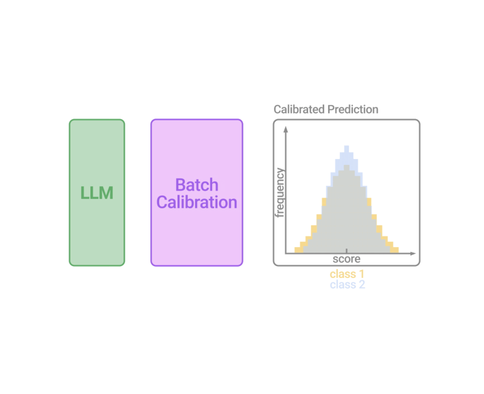
Inspired by the previous discussions, we designed BC to be a zero-shot, inference-only and generalizable calibration technique with negligible computation cost. We argue that the most critical component for calibration is to accurately estimate the contextual bias. We, therefore, opt for a linear decision boundary for its robustness, and instead of relying on content-free inputs, we propose to estimate the contextual bias for each class from a batch in a content-based manner by marginalizing the output score over all samples within the batch, which is equivalent to measuring the mean score for each class (visualized below).

We then obtain the calibrated probability by dividing the output probability over the contextual prior, which is equivalent to aligning the log-probability (LLM scores) distribution to the estimated mean of each class. It is noteworthy that because it requires no additional inputs to estimate the bias, this BC procedure is zero-shot, only involves unlabeled test samples, and incurs negligible computation costs. We may either compute the contextual bias once all test samples are seen, or alternatively, in an on-the-fly manner that dynamically processes the outputs. To do so, we may use a running estimate of the contextual bias for BC, thereby allowing BC's calibration term to be estimated from a small number of mini-batches that is subsequently stabilized when more mini-batches arrive.

Illustration of Batch Calibration (BC). Batches of demonstrations with in-context examples and test samples are passed into the LLM. Due to sources of implicit bias in the context, the score distribution from the LLM becomes biased. BC is a modular and adaptable layer option appended to the output of the LLM that generates calibrated scores (visualized for illustration only).

Experiment design

For natural language tasks, we conduct experiments on 13 more diverse and challenging classification tasks, including the standard GLUE and SuperGLUE datasets. This is in contrast to previous works that only report on relatively simple single-sentence classification tasks.. For image classification tasks, we include SVHN, EuroSAT, and CLEVR. We conduct experiments mainly on the state-of-the-art PaLM 2 with size variants PaLM 2-S, PaLM 2-M, and PaLM 2-L. For VLMs, we report the results on CLIP ViT-B/16.

Results

Notably, BC consistently outperforms ICL, yielding a significant performance enhancement of 8% and 6% on small and large variants of PaLM 2, respectively. This shows that the BC implementation successfully mitigates the contextual bias from the in-context examples and unleashes the full potential of LLM in efficient learning and quick adaptation to new tasks. In addition, BC improves over the state-of-the-art prototypical calibration (PC) baseline by 6% on PaLM 2-S, and surpasses the competitive contextual calibration (CC) baseline by another 3% on average on PaLM 2-L. Specifically, BC is a generalizable and cheaper technique across all evaluated tasks, delivering stable performance improvement, whereas previous baselines exhibit varying degrees of performance across tasks.

Batch Calibration (BC) achieves the best performance on 1-shot ICL over calibration baselines: contextual calibration (CC), domain-context calibration (DC), and prototypical calibration (PC) on an average of 13 NLP tasks on PaLM 2 and outperforms the zero-shot CLIP on image tasks.

We analyze the performance of BC by varying the number of ICL shots from 0 to 4, and BC again outperforms all baseline methods. We also observe an overall trend for improved performance when more shots are available, where BC demonstrates the best stability.

The ICL performance on various calibration techniques over the number of ICL shots on PaLM 2-S. We compare BC with the uncalibrated ICL, contextual calibration (CC), domain-context calibration (DC), and prototypical calibration (PC) baselines.

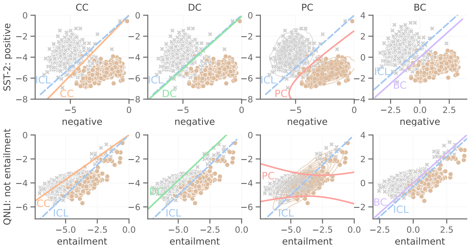
We further visualize the decision boundaries of uncalibrated ICL after applying existing calibration methods and the proposed BC. We show success and failure cases for each baseline method, whereas BC is consistently effective.

Visualization of the decision boundaries of uncalibrated ICL, and after applying existing calibration methods and the proposed BC in representative binary classification tasks of SST-2 (top row) and QNLI (bottom row) on 1-shot PaLM 2-S. Each axis indicates the LLM score on the defined label.

Robustness and ablation studies

We analyze the robustness of BC with respect to common prompt engineering design choices that were previously shown to significantly affect LLM performance: choices and orders of in-context examples, the prompt template for ICL, and the label space. First, we find that BC is more robust to ICL choices and can mostly achieve the same performance with different ICL examples. Additionally, given a single set of ICL shots, altering the order between each ICL example has minimal impact on the BC performance. Furthermore, we analyze the robustness of BC under 10 designs of prompt templates, where BC shows consistent improvement over the ICL baseline. Therefore, though BC improves performance, a well-designed template can further enhance the performance of BC. Lastly, we examine the robustness of BC to variations in label space designs (see appendix in our paper). Remarkably, even when employing unconventional choices such as emoji pairs as labels, leading to dramatic oscillations of ICL performance, BC largely recovers performance. This observation demonstrates that BC increases the robustness of LLM predictions under common prompt design choices and makes prompt engineering easier.

Batch Calibration makes prompt engineering easier while being data-efficient. Data are visualized as a standard box plot, which illustrates values for the median, first and third quartiles, and minimum and maximum.

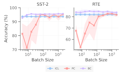
Moreover, we study the impact of batch size on the performance of BC. In contrast to PC, which also leverages an unlabeled estimate set, BC is remarkably more sample efficient, achieving a strong performance with only around 10 unlabeled samples, whereas PC requires more than 500 unlabeled samples before its performance stabilizes.

Batch Calibration makes prompt engineering easier while being insensitive to the batch size.

Conclusion

We first revisit previous calibration methods while addressing two critical research questions from an interpretation of decision boundaries, revealing their failure cases and deficiencies. We then propose Batch Calibration, a zero-shot and inference-only calibration technique. While methodologically simple and easy to implement with negligible computation cost, we show that BC scales from a language-only setup to the vision-language context, achieving state-of-the-art performance in both modalities. BC significantly improves the robustness of LLMs with respect to prompt designs, and we expect easy prompt engineering with BC.

Acknowledgements

This work was conducted by Han Zhou, Xingchen Wan, Lev Proleev, Diana Mincu, Jilin Chen, Katherine Heller, Subhrajit Roy. We would like to thank Mohammad Havaei and other colleagues at Google Research for their discussion and feedback.

Source: Google AI Blog

Symbol tuning improves in-context learning in language models

Posted by Jerry Wei, Student Researcher, and Denny Zhou, Principal Scientist, Google Research

A key feature of human intelligence is that humans can learn to perform new tasks by reasoning using only a few examples. Scaling up language models has unlocked a range of new applications and paradigms in machine learning, including the ability to perform challenging reasoning tasks via in-context learning. Language models, however, are still sensitive to the way that prompts are given, indicating that they are not reasoning in a robust manner. For instance, language models often require heavy prompt engineering or phrasing tasks as instructions, and they exhibit unexpected behaviors such as performance on tasks being unaffected even when shown incorrect labels.

In “Symbol tuning improves in-context learning in language models”, we propose a simple fine-tuning procedure that we call symbol tuning, which can improve in-context learning by emphasizing input–label mappings. We experiment with symbol tuning across Flan-PaLM models and observe benefits across various settings.

Symbol tuning boosts performance on unseen in-context learning tasks and is much more robust to underspecified prompts, such as those without instructions or without natural language labels.
Symbol-tuned models are much stronger at algorithmic reasoning tasks.
Finally, symbol-tuned models show large improvements in following flipped-labels presented in-context, meaning that they are more capable of using in-context information to override prior knowledge.

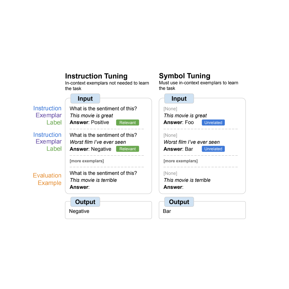
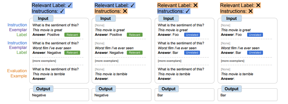
An overview of symbol tuning, where models are fine-tuned on tasks where natural language labels are replaced with arbitrary symbols. Symbol tuning relies on the intuition that when instruction and relevant labels are not available, models must use in-context examples to learn the task.

Motivation

Instruction tuning is a common fine-tuning method that has been shown to improve performance and allow models to better follow in-context examples. One shortcoming, however, is that models are not forced to learn to use the examples because the task is redundantly defined in the evaluation example via instructions and natural language labels. For example, on the left in the figure above, although the examples can help the model understand the task (sentiment analysis), they are not strictly necessary since the model could ignore the examples and just read the instruction that indicates what the task is.

In symbol tuning, the model is fine-tuned on examples where the instructions are removed and natural language labels are replaced with semantically-unrelated labels (e.g., “Foo,” “Bar,” etc.). In this setup, the task is unclear without looking at the in-context examples. For example, on the right in the figure above, multiple in-context examples would be needed to figure out the task. Because symbol tuning teaches the model to reason over the in-context examples, symbol-tuned models should have better performance on tasks that require reasoning between in-context examples and their labels.

Datasets and task types used for symbol tuning.

Symbol-tuning procedure

We selected 22 publicly-available natural language processing (NLP) datasets that we use for our symbol-tuning procedure. These tasks have been widely used in the past, and we only chose classification-type tasks since our method requires discrete labels. We then remap labels to a random label from a set of ~30K arbitrary labels selected from one of three categories: integers, character combinations, and words.

For our experiments, we symbol tune Flan-PaLM, the instruction-tuned variants of PaLM. We use three different sizes of Flan-PaLM models: Flan-PaLM-8B, Flan-PaLM-62B, and Flan-PaLM-540B. We also tested Flan-cont-PaLM-62B (Flan-PaLM-62B at 1.3T tokens instead of 780B tokens), which we abbreviate as 62B-c.

We use a set of ∼300K arbitrary symbols from three categories (integers, character combinations, and words). ∼30K symbols are used during tuning and the rest are held out for evaluation.

Experimental setup

We want to evaluate a model’s ability to perform unseen tasks, so we cannot evaluate on tasks used in symbol tuning (22 datasets) or used during instruction tuning (1.8K tasks). Hence, we choose 11 NLP datasets that were not used during fine-tuning.

In-context learning

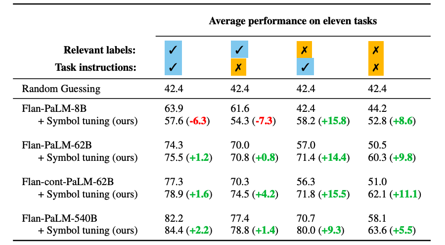
In the symbol-tuning procedure, models must learn to reason with in-context examples in order to successfully perform tasks because prompts are modified to ensure that tasks cannot simply be learned from relevant labels or instructions. Symbol-tuned models should perform better in settings where tasks are unclear and require reasoning between in-context examples and their labels. To explore these settings, we define four in-context learning settings that vary the amount of reasoning required between inputs and labels in order to learn the task (based on the availability of instructions/relevant labels)

Depending on the availability of instructions and relevant natural language labels, models may need to do varying amounts of reasoning with in-context examples. When these features are not available, models must reason with the given in-context examples to successfully perform the task.

Symbol tuning improves performance across all settings for models 62B and larger, with small improvements in settings with relevant natural language labels (+0.8% to +4.2%) and substantial improvements in settings without relevant natural language labels (+5.5% to +15.5%). Strikingly, when relevant labels are unavailable, symbol-tuned Flan-PaLM-8B outperforms FlanPaLM-62B, and symbol-tuned Flan-PaLM-62B outperforms Flan-PaLM-540B. This performance difference suggests that symbol tuning can allow much smaller models to perform as well as large models on these tasks (effectively saving ∼10X inference compute).

Large-enough symbol-tuned models are better at in-context learning than baselines, especially in settings where relevant labels are not available. Performance is shown as average model accuracy (%) across eleven tasks.

Algorithmic reasoning

We also experiment on algorithmic reasoning tasks from BIG-Bench. There are two main groups of tasks: 1) List functions — identify a transformation function (e.g., remove the last element in a list) between input and output lists containing non-negative integers; and 2) simple turing concepts — reason with binary strings to learn the concept that maps an input to an output (e.g., swapping 0s and 1s in a string).

On the list function and simple turing concept tasks, symbol tuning results in an average performance improvement of 18.2% and 15.3%, respectively. Additionally, Flan-cont-PaLM-62B with symbol tuning outperforms Flan-PaLM-540B on the list function tasks on average, which is equivalent to a ∼10x reduction in inference compute. These improvements suggest that symbol tuning strengthens the model’s ability to learn in-context for unseen task types, as symbol tuning did not include any algorithmic data.

Symbol-tuned models achieve higher performance on list function tasks and simple turing concept tasks. (A–E): categories of list functions tasks. (F): simple turing concepts task.

Flipped labels

In the flipped-label experiment, labels of in-context and evaluation examples are flipped, meaning that prior knowledge and input-label mappings disagree (e.g., sentences containing positive sentiment labeled as “negative sentiment”), thereby allowing us to study whether models can override prior knowledge. Previous work has shown that while pre-trained models (without instruction tuning) can, to some extent, follow flipped labels presented in-context, instruction tuning degraded this ability.

We see that there is a similar trend across all model sizes — symbol-tuned models are much more capable of following flipped labels than instruction-tuned models. We found that after symbol tuning, Flan-PaLM-8B sees an average improvement across all datasets of 26.5%, Flan-PaLM-62B sees an improvement of 33.7%, and Flan-PaLM-540B sees an improvement of 34.0%. Additionally, symbol-tuned models achieve similar or better than average performance as pre-training–only models.

Symbol-tuned models are much better at following flipped labels presented in-context than instruction-tuned models are.

Conclusion

We presented symbol tuning, a new method of tuning models on tasks where natural language labels are remapped to arbitrary symbols. Symbol tuning is based off of the intuition that when models cannot use instructions or relevant labels to determine a presented task, it must do so by instead learning from in-context examples. We tuned four language models using our symbol-tuning procedure, utilizing a tuning mixture of 22 datasets and approximately 30K arbitrary symbols as labels.

We first showed that symbol tuning improves performance on unseen in-context learning tasks, especially when prompts do not contain instructions or relevant labels. We also found that symbol-tuned models were much better at algorithmic reasoning tasks, despite the lack of numerical or algorithmic data in the symbol-tuning procedure. Finally, in an in-context learning setting where inputs have flipped labels, symbol tuning (for some datasets) restores the ability to follow flipped labels that was lost during instruction tuning.

Future work

Through symbol tuning, we aim to increase the degree to which models can examine and learn from input–label mappings during in-context learning. We hope that our results encourage further work towards improving language models’ ability to reason over symbols presented in-context.

Acknowledgements

The authors of this post are now part of Google DeepMind. This work was conducted by Jerry Wei, Le Hou, Andrew Lampinen, Xiangning Chen, Da Huang, Yi Tay, Xinyun Chen, Yifeng Lu, Denny Zhou, Tengyu Ma, and Quoc V. Le. We would like to thank our colleagues at Google Research and Google DeepMind for their advice and helpful discussions.

Source: Google AI Blog

Symbol tuning improves in-context learning in language models

Posted by Jerry Wei, Student Researcher, and Denny Zhou, Principal Scientist, Google Research

Symbol tuning boosts performance on unseen in-context learning tasks and is much more robust to underspecified prompts, such as those without instructions or without natural language labels.
Symbol-tuned models are much stronger at algorithmic reasoning tasks.
Finally, symbol-tuned models show large improvements in following flipped-labels presented in-context, meaning that they are more capable of using in-context information to override prior knowledge.

Motivation

Datasets and task types used for symbol tuning.

Symbol-tuning procedure

We use a set of ∼300K arbitrary symbols from three categories (integers, character combinations, and words). ∼30K symbols are used during tuning and the rest are held out for evaluation.

Experimental setup

In-context learning

Algorithmic reasoning

Symbol-tuned models achieve higher performance on list function tasks and simple turing concept tasks. (A–E): categories of list functions tasks. (F): simple turing concepts task.

Flipped labels

Symbol-tuned models are much better at following flipped labels presented in-context than instruction-tuned models are.

Conclusion

Future work

Acknowledgements

Source: Google AI Blog

Symbol tuning improves in-context learning in language models

Posted by Jerry Wei, Student Researcher, and Denny Zhou, Principal Scientist, Google Research

Symbol tuning boosts performance on unseen in-context learning tasks and is much more robust to underspecified prompts, such as those without instructions or without natural language labels.
Symbol-tuned models are much stronger at algorithmic reasoning tasks.
Finally, symbol-tuned models show large improvements in following flipped-labels presented in-context, meaning that they are more capable of using in-context information to override prior knowledge.

Motivation

Datasets and task types used for symbol tuning.

Symbol-tuning procedure

We use a set of ∼300K arbitrary symbols from three categories (integers, character combinations, and words). ∼30K symbols are used during tuning and the rest are held out for evaluation.

Experimental setup

In-context learning

Algorithmic reasoning

Symbol-tuned models achieve higher performance on list function tasks and simple turing concept tasks. (A–E): categories of list functions tasks. (F): simple turing concepts task.

Flipped labels

Symbol-tuned models are much better at following flipped labels presented in-context than instruction-tuned models are.

Conclusion

Future work

Acknowledgements

Source: Google AI Blog

Larger language models do in-context learning differently

Posted by Jerry Wei, Student Researcher, and Denny Zhou, Principal Scientist, Google Research

There have recently been tremendous advances in language models, partly because they can perform tasks with strong performance via in-context learning (ICL), a process whereby models are prompted with a few examples of input-label pairs before performing the task on an unseen evaluation example. In general, models’ success at in-context learning is enabled by:

Their use of semantic prior knowledge from pre-training to predict labels while following the format of in-context examples (e.g., seeing examples of movie reviews with “positive sentiment” and “negative sentiment” as labels and performing sentiment analysis using prior knowledge).
Learning the input-label mappings in context from the presented examples (e.g., finding a pattern that positive reviews should be mapped to one label, and negative reviews should be mapped to a different label).

In “Larger language models do in-context learning differently”, we aim to learn about how these two factors (semantic priors and input-label mappings) interact with each other in ICL settings, especially with respect to the scale of the language model that’s used. We investigate two settings to study these two factors — ICL with flipped labels (flipped-label ICL) and ICL with semantically-unrelated labels (SUL-ICL). In flipped-label ICL, labels of in-context examples are flipped so that semantic priors and input-label mappings disagree with each other. In SUL-ICL, labels of in-context examples are replaced with words that are semantically unrelated to the task presented in-context. We found that overriding prior knowledge is an emergent ability of model scale, as is the ability to learn in-context with semantically-unrelated labels. We also found that instruction tuning strengthens the use of prior knowledge more than it increases the capacity to learn input-label mappings.

An overview of flipped-label ICL and semantically-unrelated label ICL (SUL-ICL), compared with regular ICL, for a sentiment analysis task. Flipped-label ICL uses flipped labels, forcing the model to override semantic priors in order to follow the in-context examples. SUL-ICL uses labels that are not semantically related to the task, which means that models must learn input-label mappings in order to perform the task because they can no longer rely on the semantics of natural language labels.

Experiment design

For a diverse dataset mixture, we experiment on seven natural language processing (NLP) tasks that have been widely used: sentiment analysis, subjective/objective classification, question classification, duplicated-question recognition, entailment recognition, financial sentiment analysis, and hate speech detection. We test five language model families, PaLM, Flan-PaLM, GPT-3, InstructGPT, and Codex.

Flipped labels

In this experiment, labels of in-context examples are flipped, meaning that prior knowledge and input-label mappings disagree (e.g., sentences containing positive sentiment labeled as “negative sentiment”), thereby allowing us to study whether models can override their priors. In this setting, models that are able to override prior knowledge and learn input-label mappings in-context should experience a decrease in performance (since ground-truth evaluation labels are not flipped).

The ability to override semantic priors when presented with flipped in-context example labels emerges with model scale. Smaller models cannot flip predictions to follow flipped labels (performance only decreases slightly), while larger models can do so (performance decreases to well below 50%).

We found that when no labels are flipped, larger models have better performance than smaller models (as expected). But when we flip more and more labels, the performance of small models stays relatively flat, but large models experience large performance drops to well-below random guessing (e.g., 90% → 22.5% for code-davinci-002).

These results indicate that large models can override prior knowledge from pre-training when contradicting input-label mappings are presented in-context. Small models can’t do this, making this ability an emergent phenomena of model scale.

Semantically-unrelated labels

In this experiment, we replace labels with semantically-irrelevant ones (e.g., for sentiment analysis, we use “foo/bar” instead of “negative/positive”), which means that the model can only perform ICL by learning from input-label mappings. If a model mostly relies on prior knowledge for ICL, then its performance should decrease after this change since it will no longer be able to use semantic meanings of labels to make predictions. A model that can learn input–label mappings in-context, on the other hand, would be able to learn these semantically-unrelated mappings and should not experience a major drop in performance.

Small models rely more on semantic priors than large models do, as indicated by the greater decrease in performance for small models than for large models when using semantically-unrelated labels (i.e., targets) instead of natural language labels. For each plot, models are shown in order of increasing model size (e.g., for GPT-3 models, a is smaller than b, which is smaller than c).

Indeed, we see that using semantically-unrelated labels results in a greater performance drop for small models. This suggests that smaller models primarily rely on their semantic priors for ICL rather than learning from the presented input-label mappings. Large models, on the other hand, have the ability to learn input-label mappings in-context when the semantic nature of labels is removed.

We also find that including more in-context examples (i.e., exemplars) results in a greater performance improvement for large models than it does for small models, indicating that large models are better at learning from in-context examples than small models are.

In the SUL-ICL setup, larger models benefit more from additional examples than smaller models do.

Instruction tuning

Instruction tuning is a popular technique for improving model performance, which involves tuning models on various NLP tasks that are phrased as instructions (e.g., “Question: What is the sentiment of the following sentence, ‘This movie is great.’ Answer: Positive”). Since the process uses natural language labels, however, an open question is whether it improves the ability to learn input-label mappings or whether it strengthens the ability to recognize and apply semantic prior knowledge. Both of these would lead to an improvement in performance on standard ICL tasks, so it’s unclear which of these occur.

We study this question by running the same two setups as before, only this time we focus on comparing standard language models (specifically, PaLM) with their instruction-tuned variants (Flan-PaLM).

First, we find that Flan-PaLM is better than PaLM when we use semantically-unrelated labels. This effect is very prominent in small models, as Flan-PaLM-8B outperforms PaLM-8B by 9.6% and almost catches up to PaLM-62B. This trend suggests that instruction tuning strengthens the ability to learn input-label mappings, which isn’t particularly surprising.

Instruction-tuned language models are better at learning input–label mappings than pre-training–only language models are.

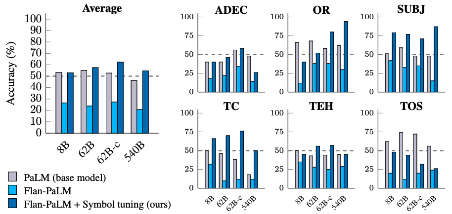
More interestingly, we saw that Flan-PaLM is actually worse than PaLM at following flipped labels, meaning that the instruction tuned models were unable to override their prior knowledge (Flan-PaLM models don’t reach below random guessing with 100% flipped labels, but PaLM models without instruction tuning can reach 31% accuracy in the same setting). These results indicate that instruction tuning must increase the extent to which models rely on semantic priors when they’re available.

Instruction-tuned models are worse than pre-training–only models at learning to override semantic priors when presented with flipped labels in-context.

Combined with the previous result, we conclude that although instruction tuning improves the ability to learn input-label mappings, it strengthens the usage of semantic prior knowledge more.

Conclusion

We examined the extent to which language models learn in-context by utilizing prior knowledge learned during pre-training versus input-label mappings presented in-context.

We first showed that large language models can learn to override prior knowledge when presented with enough flipped labels, and that this ability emerges with model scale. We then found that successfully doing ICL using semantically-unrelated labels is another emergent ability of model scale. Finally, we analyzed instruction-tuned language models and saw that instruction tuning improves the capacity to learn input-label mappings but also strengthens the use of semantic prior knowledge even more.

Future work

These results underscore how the ICL behavior of language models can change depending on their scale, and that larger language models have an emergent ability to map inputs to many types of labels, a form of reasoning in which input-label mappings can potentially be learned for arbitrary symbols. Future research could help provide insights on why these phenomena occur with respect to model scale.

Acknowledgements

This work was conducted by Jerry Wei, Jason Wei, Yi Tay, Dustin Tran, Albert Webson, Yifeng Lu, Xinyun Chen, Hanxiao Liu, Da Huang, Denny Zhou, and Tengyu Ma. We would like to thank Sewon Min and our fellow collaborators at Google Research for their advice and helpful discussions.

Source: Google AI Blog

Unsupervised and semi-supervised anomaly detection with data-centric ML

Posted by Jinsung Yoon and Sercan O. Arik, Research Scientists, Google Research, Cloud AI Team

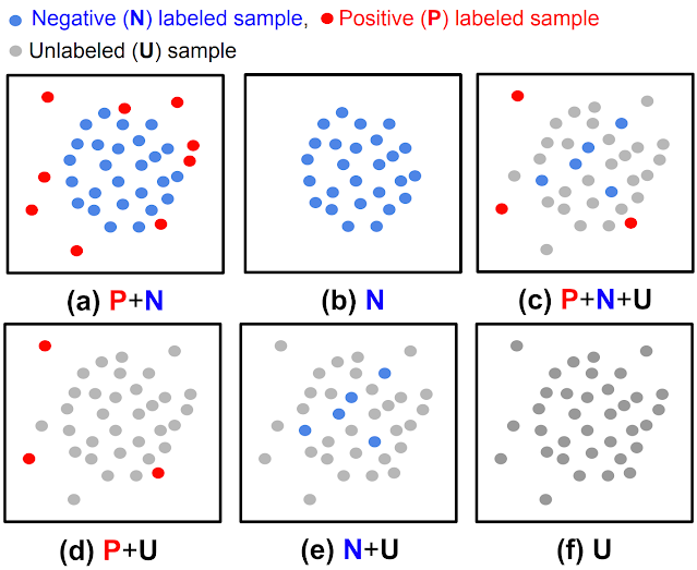
Anomaly detection (AD), the task of distinguishing anomalies from normal data, plays a vital role in many real-world applications, such as detecting faulty products from vision sensors in manufacturing, fraudulent behaviors in financial transactions, or network security threats. Depending on the availability of the type of data — negative (normal) vs. positive (anomalous) and the availability of their labels — the task of AD involves different challenges.

(a) Fully supervised anomaly detection, (b) normal-only anomaly detection, (c, d, e) semi-supervised anomaly detection, (f) unsupervised anomaly detection.

While most previous works were shown to be effective for cases with fully-labeled data (either (a) or (b) in the above figure), such settings are less common in practice because labels are particularly tedious to obtain. In most scenarios users have a limited labeling budget, and sometimes there aren’t even any labeled samples during training. Furthermore, even when labeled data are available, there could be biases in the way samples are labeled, causing distribution differences. Such real-world data challenges limit the achievable accuracy of prior methods in detecting anomalies.

This post covers two of our recent papers on AD, published in Transactions on Machine Learning Research (TMLR), that address the above challenges in unsupervised and semi-supervised settings. Using data-centric approaches, we show state-of-the-art results in both. In “Self-supervised, Refine, Repeat: Improving Unsupervised Anomaly Detection”, we propose a novel unsupervised AD framework that relies on the principles of self-supervised learning without labels and iterative data refinement based on the agreement of one-class classifier (OCC) outputs. In “SPADE: Semi-supervised Anomaly Detection under Distribution Mismatch”, we propose a novel semi-supervised AD framework that yields robust performance even under distribution mismatch with limited labeled samples.

Unsupervised anomaly detection with SRR: Self-supervised, Refine, Repeat

Discovering a decision boundary for a one-class (normal) distribution (i.e., OCC training) is challenging in fully unsupervised settings as unlabeled training data include two classes (normal and abnormal). The challenge gets further exacerbated as the anomaly ratio gets higher for unlabeled data. To construct a robust OCC with unlabeled data, excluding likely-positive (anomalous) samples from the unlabeled data, the process referred to as data refinement, is critical. The refined data, with a lower anomaly ratio, are shown to yield superior anomaly detection models.

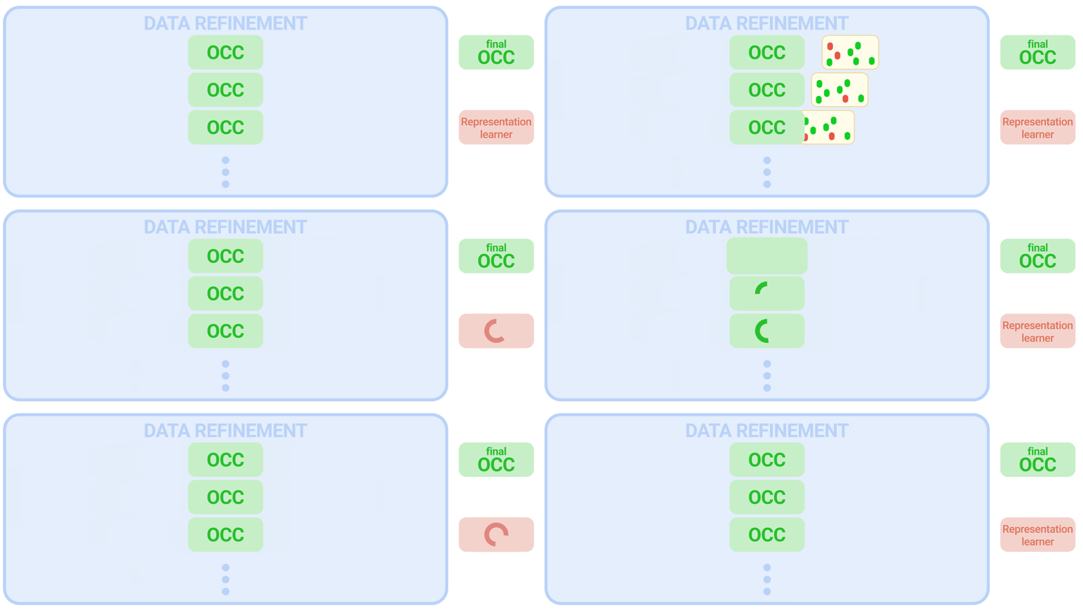
SRR first refines data from an unlabeled dataset, then iteratively trains deep representations using refined data while improving the refinement of unlabeled data by excluding likely-positive samples. For data refinement, an ensemble of OCCs is employed, each of which is trained on a disjoint subset of unlabeled training data. If there is consensus among all the OCCs in the ensemble, the data that are predicted to be negative (normal) are included in the refined data. Finally, the refined training data are used to train the final OCC to generate the anomaly predictions.

Training SRR with a data refinement module (OCCs ensemble), representation learner, and final OCC. (Green/red dots represent normal/abnormal samples, respectively).

SRR results

We conduct extensive experiments across various datasets from different domains, including semantic AD (CIFAR-10, Dog-vs-Cat), real-world manufacturing visual AD (MVTec), and real-world tabular AD benchmarks such as detecting medical (Thyroid) or network security (KDD 1999) anomalies. We consider methods with both shallow (e.g., OC-SVM) and deep (e.g., GOAD, CutPaste) models. Since the anomaly ratio of real-world data can vary, we evaluate models at different anomaly ratios of unlabeled training data and show that SRR significantly boosts AD performance. For example, SRR improves more than 15.0 average precision (AP) with a 10% anomaly ratio compared to a state-of-the-art one-class deep model on CIFAR-10. Similarly, on MVTec, SRR retains solid performance, dropping less than 1.0 AUC with a 10% anomaly ratio, while the best existing OCC drops more than 6.0 AUC. Lastly, on Thyroid (tabular data), SRR outperforms a state-of-the-art one-class classifier by 22.9 F1 score with a 2.5% anomaly ratio.

Across various domains, SRR (blue line) significantly boosts AD performance with various anomaly ratios in fully unsupervised settings.

SPADE: Semi-supervised Pseudo-labeler Anomaly Detection with Ensembling

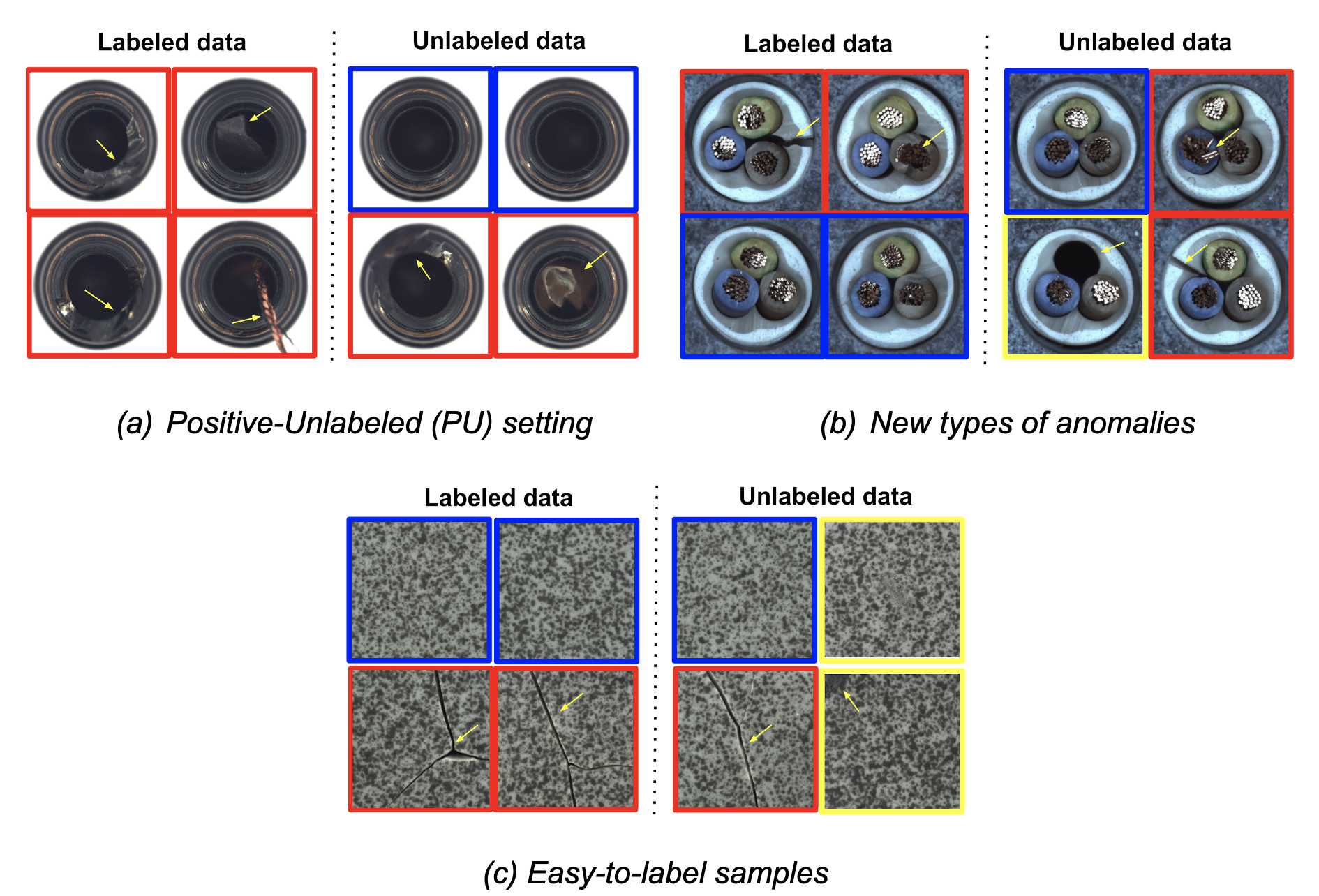
Most semi-supervised learning methods (e.g., FixMatch, VIME) assume that the labeled and unlabeled data come from the same distributions. However, in practice, distribution mismatch commonly occurs, with labeled and unlabeled data coming from different distributions. One such case is positive and unlabeled (PU) or negative and unlabeled (NU) settings, where the distributions between labeled (either positive or negative) and unlabeled (both positive and negative) samples are different. Another cause of distribution shift is additional unlabeled data being gathered after labeling. For example, manufacturing processes may keep evolving, causing the corresponding defects to change and the defect types at labeling to differ from the defect types in unlabeled data. In addition, for applications like financial fraud detection and anti-money laundering, new anomalies can appear after the data labeling process, as criminal behavior may adapt. Lastly, labelers are more confident on easy samples when they label them; thus, easy/difficult samples are more likely to be included in the labeled/unlabeled data. For example, with some crowd-sourcing–based labeling, only the samples with some consensus on the labels (as a measure of confidence) are included in the labeled set.

Three common real-world scenarios with distribution mismatches (blue box: normal samples, red box: known/easy anomaly samples, yellow box: new/difficult anomaly samples).

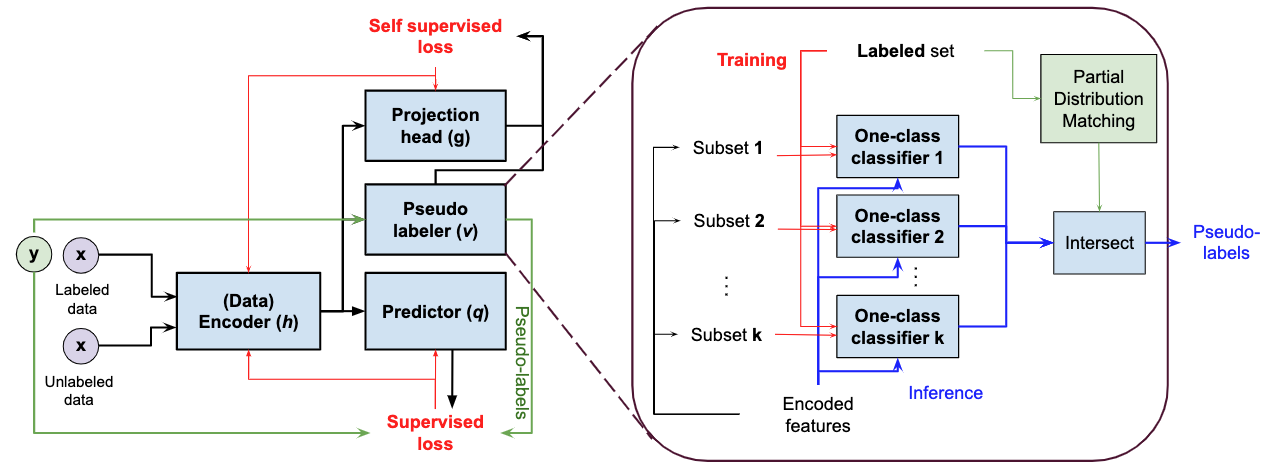
Standard semi-supervised learning methods assume that labeled and unlabeled data come from the same distribution, so are sub-optimal for semi-supervised AD under distribution mismatch. SPADE utilizes an ensemble of OCCs to estimate the pseudo-labels of the unlabeled data — it does this independent of the given positive labeled data, thus reducing the dependency on the labels. This is especially beneficial when there is a distribution mismatch. In addition, SPADE employs partial matching to automatically select the critical hyper-parameters for pseudo-labeling without relying on labeled validation data, a crucial capability given limited labeled data.

Block diagram of SPADE with zoom in the detailed block diagram of the proposed pseudo-labelers.

SPADE results

We conduct extensive experiments to showcase the benefits of SPADE in various real-world settings of semi-supervised learning with distribution mismatch. We consider multiple AD datasets for image (including MVTec) and tabular (including Covertype, Thyroid) data.

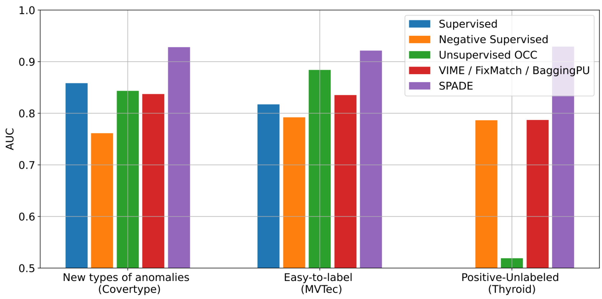
SPADE shows state-of-the-art semi-supervised anomaly detection performance across a wide range of scenarios: (i) new-types of anomalies, (ii) easy-to-label samples, and (iii) positive-unlabeled examples. As shown below, with new-types of anomalies, SPADE outperforms the state-of-the-art alternatives by 5% AUC on average.

AD performances with three different scenarios across various datasets (Covertype, MVTec, Thyroid) in terms of AUC. Some baselines are only applicable to some scenarios. More results with other baselines and datasets can be found in the paper.

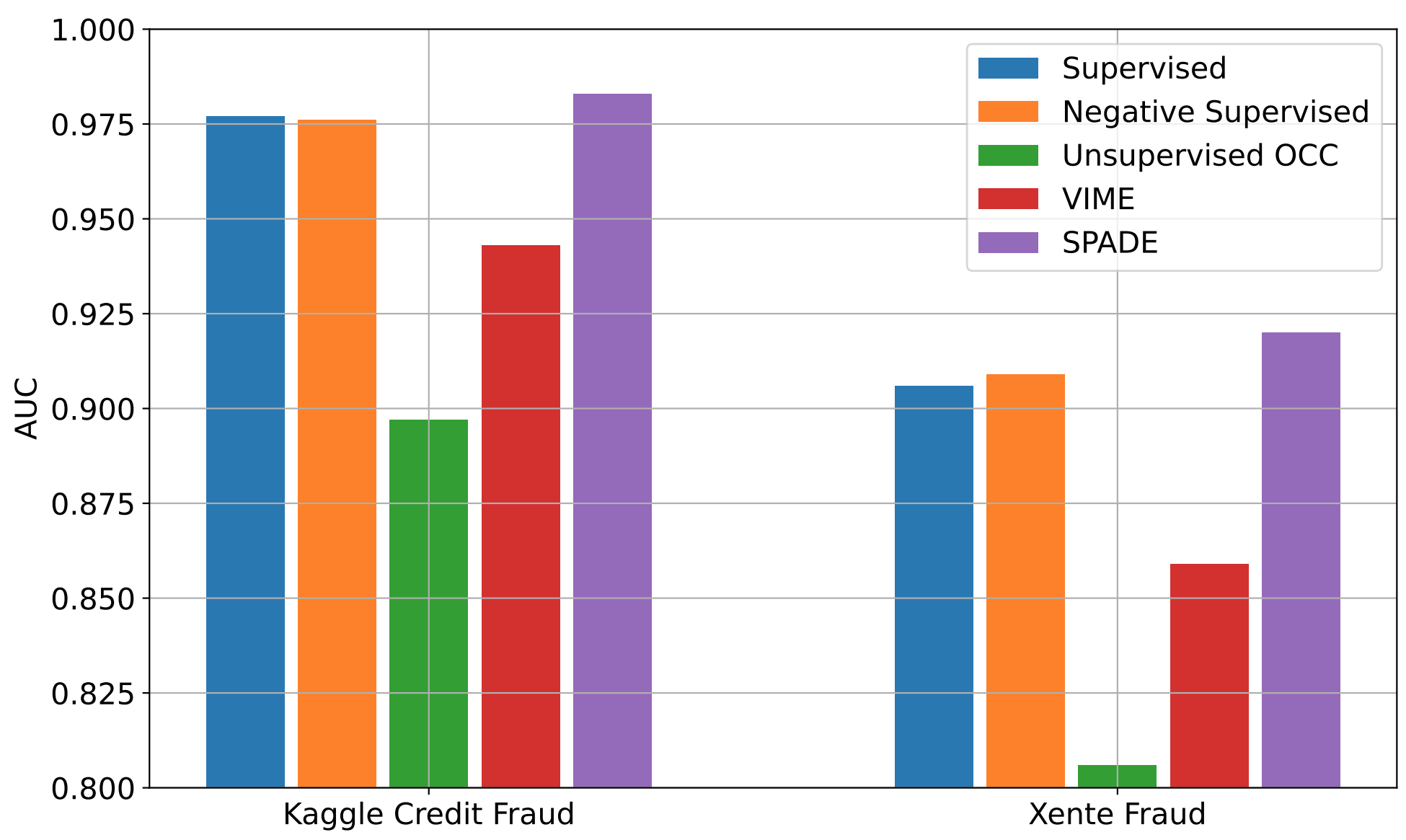
We also evaluate SPADE on real-world financial fraud detection datasets: Kaggle credit card fraud and Xente fraud detection. For these, anomalies evolve (i.e., their distributions change over time) and to identify evolving anomalies, we need to keep labeling for new anomalies and retrain the AD model. However, labeling would be costly and time consuming. Even without additional labeling, SPADE can improve the AD performance using both labeled data and newly-gathered unlabeled data.

AD performances with time-varying distributions using two real-world fraud detection datasets with 10% labeling ratio. More baselines can be found in the paper.

As shown above, SPADE consistently outperforms alternatives on both datasets, taking advantage of the unlabeled data and showing robustness to evolving distributions.

Conclusions

AD has a wide range of use cases with significant importance in real-world applications, from detecting security threats in financial systems to identifying faulty behaviors of manufacturing machines.

One challenging and costly aspect of building an AD system is that anomalies are rare and not easily detectable by people. To this end, we have proposed SRR, a canonical AD framework to enable high performance AD without the need for manual labels for training. SRR can be flexibly integrated with any OCC, and applied on raw data or on trainable representations.

Semi-supervised AD is another highly-important challenge — in many scenarios, the distributions of labeled and unlabeled samples don’t match. SPADE introduces a robust pseudo-labeling mechanism using an ensemble of OCCs and a judicious way of combining supervised and self-supervised learning. In addition, SPADE introduces an efficient approach to pick critical hyperparameters without a validation set, a crucial component for data-efficient AD.

Overall, we demonstrate that SRR and SPADE consistently outperform the alternatives in various scenarios across multiple types of datasets.

Acknowledgements

We gratefully acknowledge the contributions of Kihyuk Sohn, Chun-Liang Li, Chen-Yu Lee, Kyle Ziegler, Nate Yoder, and Tomas Pfister.

Source: Google AI Blog

Discovering Anomalous Data with Self-Supervised Learning

Posted by Kihyuk Sohn and Chun-Liang Li, Research Scientists, Google Cloud

Anomaly detection (sometimes called outlier detection or out-of-distribution detection) is one of the most common machine learning applications across many domains, from defect detection in manufacturing to fraudulent transaction detection in finance. It is most often used when it is easy to collect a large amount of known-normal examples but where anomalous data is rare and difficult to find. As such, one-class classification, such as one-class support vector machine (OC-SVM) or support vector data description (SVDD), is particularly relevant to anomaly detection because it assumes the training data are all normal examples, and aims to identify whether an example belongs to the same distribution as the training data. Unfortunately, these classical algorithms do not benefit from the representation learning that makes machine learning so powerful. On the other hand, substantial progress has been made in learning visual representations from unlabeled data via self-supervised learning, including rotation prediction and contrastive learning. As such, combining one-class classifiers with these recent successes in deep representation learning is an under-explored opportunity for the detection of anomalous data.

In “Learning and Evaluating Representations for Deep One-class Classification”, presented at ICLR 2021, we outline a 2-stage framework that makes use of recent progress on self-supervised representation learning and classic one-class algorithms. The algorithm is simple to train and results in state-of-the-art performance on various benchmarks, including CIFAR, f-MNIST, Cat vs Dog and CelebA. We then follow up on this in “CutPaste: Self-Supervised Learning for Anomaly Detection and Localization”, presented at CVPR 2021, in which we propose a new representation learning algorithm under the same framework for a realistic industrial defect detection problem. The framework achieves a new state-of-the-art on the MVTec benchmark.

A Two-Stage Framework for Deep One-Class Classification
While end-to-end learning has demonstrated success in many machine learning problems, including deep learning algorithm designs, such an approach for deep one-class classifiers often suffer from degeneration in which the model outputs the same results regardless of the input.

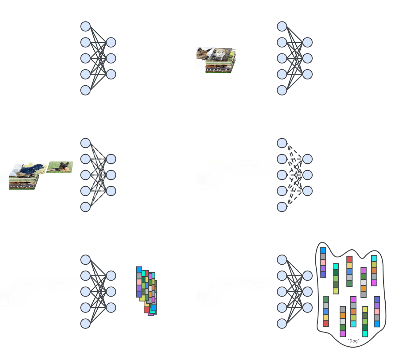
To combat this, we apply a two stage framework. In the first stage, the model learns deep representations with self-supervision. In the second stage, we adopt one-class classification algorithms, such as OC-SVM or kernel density estimator, using the learned representations from the first stage. This 2-stage algorithm is not only robust to degeneration, but also enables one to build more accurate one-class classifiers. Furthermore, the framework is not limited to specific representation learning and one-class classification algorithms — that is, one can easily plug-and-play different algorithms, which is useful if any advanced approaches are developed.

A deep neural network is trained to generate the representations of input images via self-supervision. We then train one-class classifiers on the learned representations.

Semantic Anomaly Detection
We test the efficacy of our 2-stage framework for anomaly detection by experimenting with two representative self-supervised representation learning algorithms, rotation prediction and contrastive learning.

Rotation prediction refers to a model’s ability to predict the rotated angles of an input image. Due to its promising performance in other computer vision applications, the end-to-end trained rotation prediction network has been widely adopted for one-class classification research. The existing approach typically reuses the built-in rotation prediction classifier for learning representations to conduct anomaly detection, which is suboptimal because those built-in classifiers are not trained for one-class classification.

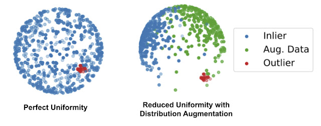
In contrastive learning, a model learns to pull together representations from transformed versions of the same image, while pushing representations of different images away. During training, as images are drawn from the dataset, each is transformed twice with simple augmentations (e.g., random cropping or color changing). We minimize the distance of the representations from the same image to encourage consistency and maximize the distance between different images. However, usual contrastive learning converges to a solution where all the representations of normal examples are uniformly spread out on a sphere. This is problematic because most of the one-class algorithms determine the outliers by checking the proximity of a tested example to the normal training examples, but when all the normal examples are uniformly distributed in an entire space, outliers will always appear close to some normal examples.

To resolve this, we propose distribution augmentation (DA) for one-class contrastive learning. The idea is that instead of learning representations from the training data only, the model learns from the union of the training data plus augmented training examples, where the augmented examples are considered to be different from the original training data. We employ geometric transformations, such as rotation or horizontal flip, for distribution augmentation. With DA, the training data is no longer uniformly distributed in the representation space because some areas are occupied by the augmented data.

Left: Illustrated examples of perfect uniformity from the standard contrastive learning. Right: The reduced uniformity by the proposed distribution augmentation (DA), where the augmented data occupy the space to avoid the uniform distribution of the inlier examples (blue) throughout the whole sphere.

We evaluate the performance of one-class classification in terms of the area under receiver operating characteristic curve (AUC) on the commonly used datasets in computer vision, including CIFAR10 and CIFAR-100, Fashion MNIST, and Cat vs Dog. Images from one class are given as inliers and those from remaining classes are given as outliers. For example, we see how well cat images are detected as anomalies when dog images are inliers.

	CIFAR-10	CIFAR-100	f-MNIST	Cat v.s. Dog
Ruff et al. (2018)	64.8	-	-	-
Golan and El-Yaniv (2018)	86.0	78.7	93.5	88.8
Bergman and Hoshen (2020)	88.2	-	94.1	-
Hendrycks et al. (2019)	90.1	-	-	-
Huang et al. (2019)	86.6	78.8	93.9	-
2-stage framework: rotation prediction	91.3±0.3	84.1±0.6	95.8±0.3	86.4±0.6
2-stage framework: contrastive (DA)	92.5±0.6	86.5±0.7	94.8±0.3	89.6±0.5

Performance comparison of one-class classification methods. Values are the mean AUCs and their standard deviation over 5 runs. AUC ranges from 0 to 100, where 100 is perfect detection.

Given the suboptimal built-in rotation prediction classifiers typically used for rotation prediction approaches, it’s notable that simply replacing the built-in rotation classifier used in the first stage for learning representations with a one-class classifier at the second stage of the proposed framework significantly boosts the performance, from 86 to 91.3 AUC. More generally, the 2-stage framework achieves state-of-the-art performance on all of the above benchmarks.

With classic OC-SVM, which learns the area boundary of representations of normal examples, the 2-stage framework results in higher performance than existing works as measured by image-level AUC.

Texture Anomaly Detection for Industrial Defect Detection
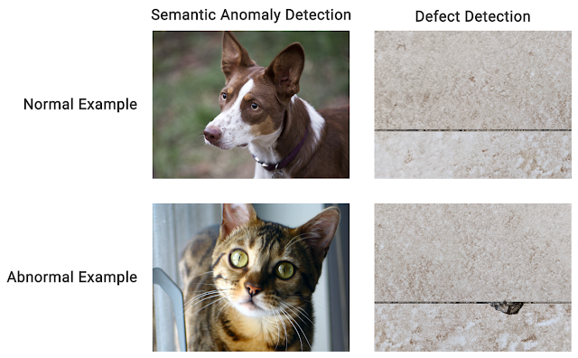
In many real-world applications of anomaly detection, the anomaly is often defined by localized defects instead of entirely different semantics (i.e., being different in general). For example, the detection of texture anomalies is useful for detecting various kinds of industrial defects.

The examples of semantic anomaly detection and defect detection. In semantic anomaly detection, the inlier and outlier are different in general, (e.g., one is a dog, the other a cat). In defect detection, the semantics for inlier and outlier are the same (e.g., they are both tiles), but the outlier has a local anomaly.

While learning representations with rotation prediction and distribution-augmented contrastive learning have demonstrated state-of-the-art performance on semantic anomaly detection, those algorithms do not perform well on texture anomaly detection. Instead, we explored different representation learning algorithms that better fit the application.

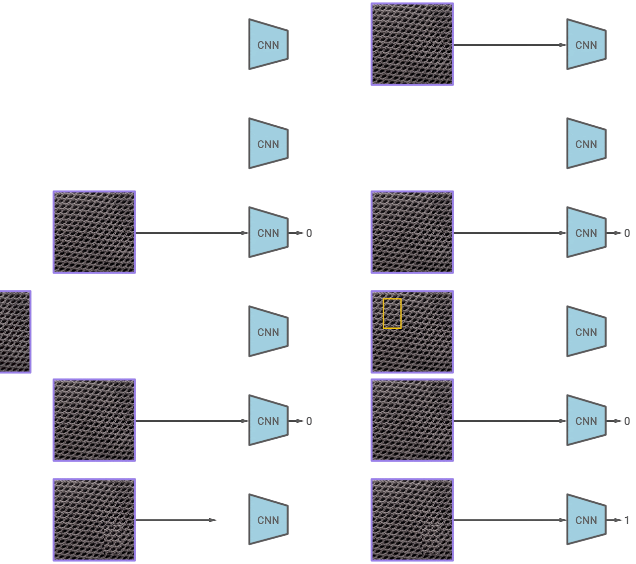
In our second paper, we propose a new self-supervised learning algorithm for texture anomaly detection. The overall anomaly detection follows the 2-stage framework, but the first stage, in which the model learns deep image representations, is specifically trained to predict whether the image is augmented via a simple CutPaste data augmentation. The idea of CutPaste augmentation is simple — a given image is augmented by randomly cutting a local patch and pasting it back to a different location of the same image. Learning to distinguish normal examples from CutPaste-augmented examples encourages representations to be sensitive to local irregularity of an image.

The illustration of learning representations by predicting CutPaste augmentations. Given an example, the CutPaste augmentation crops a local patch, then pasties it to a randomly selected area of the same image. We then train a binary classifier to distinguish the original image and the CutPaste augmented image.

We use MVTec, a real-world defect detection dataset with 15 object categories, to evaluate the approach above.

DOCC (Ruff et al., 2020)	U-Student (Bergmann et al., 2020)	Rotation Prediction	Contrastive (DA)	CutPaste
87.9	92.5	86.3	86.5	95.2

Image-level anomaly detection performance (in AUC) on the MVTec benchmark.

Besides image-level anomaly detection, we use the CutPaste method to locate where the anomaly is, i.e., “patch-level” anomaly detection. We aggregate the patch anomaly scores via upsampling with Gaussian smoothing and visualize them in heatmaps that show where the anomaly is. Interestingly, this provides decently improved localization of anomalies. The below table shows the pixel-level AUC for localization evaluation.

Autoencoder (Bergmann et al., 2019)	FCDD (Ruff et al., 2020)	Rotation Prediction	Contrastive (DA)	CutPaste
86.0	92.0	93.0	90.4	96.0

Pixel-level anomaly localization performance (in AUC) comparison between different algorithms on the MVTec benchmark.

Conclusion
In this work we introduce a novel 2-stage deep one-class classification framework and emphasize the importance of decoupling building classifiers from learning representations so that the classifier can be consistent with the target task, one-class classification. Moreover, this approach permits applications of various self-supervised representation learning methods, attaining state-of-the-art performance on various applications of visual one-class classification from semantic anomaly to texture defect detection. We are extending our efforts to build more realistic anomaly detection methods under the scenario where training data is truly unlabeled.

Acknowledgements
We gratefully acknowledge the contribution from other co-authors, including Jinsung Yoon, Minho Jin and Tomas Pfister. We release the code in our GitHub repository.

Source: Google AI Blog

RxR: A Multilingual Benchmark for Navigation Instruction Following

Posted by Alexander Ku, Software Engineer and Peter Anderson, Research Scientist, Google Research

A core challenge in machine learning (ML) is to build agents that can navigate complex human environments in response to spoken or written commands. While today’s agents, including robots, can often navigate complicated environments, they cannot yet understand navigation goals expressed in natural language, such as, “Go past the brown double doors that are closed to your right and stand behind the chair at the head of the table.”

This challenge, referred to as vision-and-language navigation (VLN), demands a sophisticated understanding of spatial language. For example, the ability to identify the position “behind the chair at the head of the table” requires finding the table, identifying which part of the table is considered to be the “head”, finding the chair closest to the head, identifying the area behind this chair and so on. While people can follow these instructions easily, these challenges cannot be easily solved with current ML-based methods, requiring systems that can better connect language to the physical world it describes.

To help spur progress in this area, we are excited to introduce Room-Across-Room (RxR), a new dataset for VLN. Described in “Room-Across-Room: Multilingual Vision-and-Language Navigation with Dense Spatiotemporal Grounding”, RxR is the first multilingual dataset for VLN, containing 126,069 human-annotated navigation instructions in three typologically diverse languages — English, Hindi and Telugu. Each instruction describes a path through a photorealistic simulator populated with indoor environments from the Matterport3D dataset, which includes 3D captures of homes, offices and public buildings. To track progress on VLN, we are also announcing the RxR Challenge, a competition that encourages the machine learning community to train and evaluate their own instruction following agents on RxR instructions.

*Language*	*Instruction*
en-US	Starting next to the long dining room table, turn so the table is to your right. Walk towards the glass double doors. When you reach the mat before the doors, turn immediately left and walk down the stairs. When you reach the bottom of the stairs, walk through the open doors to your left and continue through the art exhibit with the tub to your right hand side. Down the length of the table until you reach the small step at the end of the room before you reach the tub and stop.

hi-IN	अभी हमारे बायीं ओर एक बड़ा मेज़ है कुछ कुर्सियाँ हैं और कुछ दीपक मेज़ के ऊपर रखे हैं। उलटी दिशा में घूम जाएँ और सिधा चलें। अभी हमारे दायीं ओर एक गोल मेज़ है वहां से सीधा बढ़ें और सामने एक शीशे का बंद दरवाज़ा है उससे पहले बायीं ओर एक सीढ़ी है उससे निचे उतरें। निचे उतरने के बाद दायीं ओर मुड़े और एक भूरे रंग के दरवाज़े से अंदर प्रवेश करें और सीधा चलें। अभी हमारे दायीं ओर एक बड़ा मेज़ है और दो कुर्सियां राखी हैं सीधा आगे बढ़ें। हमारे सामने एक पानी का कल है और सामने तीन कुर्सियां दिवार के पास रखी हैं यहीं पर ठहर जाएँ।

te-IN	ఉన్న చోటు నుండి వెనకకు తిరిగి, నేరుగా వెళ్తే, మీ ముందర ఒక బల్ల ఉంటుంది. దాన్ని దాటుకొని ఎడమవైపుకి తిరిగితే, మీ ముందర మెట్లు ఉంటాయి. వాటిని పూర్తిగా దిగండి. ఇప్పుడు మీ ముందర రెండు తెరిచిన ద్వారాలు ఉంటాయి. ఎడమవైపు ఉన్న ద్వారం గుండా బయటకు వెళ్ళి, నేరుగా నడవండి. ఇప్పుడు మీ కుడివైపున పొడవైన బల్ల ఉంటుంది. దాన్ని దాటుకొని ముందరే ఉన్న మెట్ల వద్దకు వెళ్ళి ఆగండి.

Examples of English, Hindi and Telugu navigation instructions from the RxR dataset. Each navigation instruction describes the same path.

Pose Traces
In addition to navigation instructions and paths, RxR also includes a new, more detailed multimodal annotation called a pose trace. Inspired by the mouse traces captured in the Localized Narratives dataset, pose traces provide dense groundings between language, vision and movement in a rich 3D setting. To generate navigation instructions, we ask guide annotators to move along a path in the simulator while narrating the path based on the surroundings. The pose trace is a record of everything the guide sees along the path, time-aligned with the words in the navigation instructions. These traces are then paired with pose traces from follower annotators, who are tasked with following the intended path by listening to the guide’s audio, thereby validating the quality of the navigation instructions. Pose traces implicitly capture notions of landmark selection and visual saliency, and represent a play-by-play account of how to solve the navigation instruction generation task (for guides) and the navigation instruction following task (for followers).

Example English navigation instruction in the RxR dataset. Words in the instruction text (right) are color-coded to align with the pose trace (left) that illustrates the movements and visual percepts of the guide annotator as they move through the environment describing the path.

The same RxR example with words in the navigation instruction aligned to 360° images along the path. The parts of the scene the guide annotator observed are highlighted; parts of the scene ignored by the annotator are faded. Red and yellow boxes highlight some of the close alignments between the textual instructions and the annotator's visual cues. The red cross indicates the next direction the annotator moved.

Scale
In total, RxR contains almost 10 million words, making it around 10 times larger than existing datasets, such as R2R and Touchdown/Retouchdown. This is important because, in comparison to tasks based on static image and text data, language tasks that require learning through movement or interaction with an environment typically suffer from a lack of large-scale training data. RxR also addresses known biases in the construction of the paths that have arisen in other datasets, such as R2R in which all paths have similar lengths and take the shortest route to the goal. In contrast, the paths in RxR are on average longer and less predictable, making them more challenging to follow and encouraging models trained on the dataset to place greater emphasis on the role of language in the task. The size, scope and detail of RxR will expand the frontier for research on grounded language learning while reducing the dominance of high resource languages such as English.

Left: RxR is an order of magnitude larger than similar existing datasets. Right: Compared to R2R, the paths in RxR are typically longer and less predictable, making them more challenging to follow.

Baselines
To better characterize and understand the RxR dataset, we trained a variety of agents on RxR using our open source framework VALAN, and language representations from the multilingual BERT model. We found that results were improved by including follower annotations as well as guide annotations during training, and that independently trained monolingual agents outperformed a single multilingual agent.

Conceptually, evaluation of these agents is straightforward — did the agent follow the intended path? Empirically, we measure the similarity between the path taken by the VLN agent and the reference path using NDTW, a normalized measure of path fidelity that ranges between 100 (perfect correspondence) and 0 (completely wrong). The average score for the follower annotators across all three languages is 79.5, due to natural variation between similar paths. In contrast, the best model (a composite of three independently trained monolingual agents, one for each language) achieved an NDTW score on the RxR test set of 41.5. While this is much better than random (15.4), it remains far below human performance. Although advances in language modeling continue to rapidly erode the headroom for improvement in text-only language understanding benchmarks such as GLUE and SuperGLUE, benchmarks like RxR that connect language to the physical world offer substantial room for improvement.

Results for our multilingual and monolingual instruction following agents on the RxR test-standard split. While performance is much better than a random walk, there remains considerable headroom to reach human performance on this task.

Competition
To encourage further research in this area, we are launching the RxR Challenge, an ongoing competition for the machine learning community to develop computational agents that can follow natural language navigation instructions. To take part, participants upload the navigation paths taken by their agent in response to the provided RxR test instructions. In the most difficult setting (reported here and in the paper), all the test environments are previously unseen. However, we also allow for settings in which the agent is either trained in or explores the test environments in advance. For more details and the latest results please visit the challenge website.

PanGEA
We are also releasing the custom web-based annotation tool that we developed to collect the RxR dataset. The Panoramic Graph Environment Annotation toolkit (PanGEA), is a lightweight and customizable codebase for collecting speech and text annotations in panoramic graph environments, such as Matterport3D and StreetLearn. It includes speech recording and virtual pose tracking, as well as tooling to align the resulting pose trace with a manual transcript. For more details please visit the PanGEA github page.

Acknowledgements
The authors would like to thank Roma Patel, Eugene Ie and Jason Baldridge for their contributions to this research. We would also like to thank all the annotators, Sneha Kudugunta for analyzing the Telugu annotations, and Igor Karpov, Ashwin Kakarla and Christina Liu for their tooling and annotation support for this project, Austin Waters and Su Wang for help with image features, and Daphne Luong for executive support for the data collection.

Source: Google AI Blog

Estimating the Impact of Training Data with Reinforcement Learning

Posted by Jinsung Yoon and Sercan O. Arik, Research Scientists, Cloud AI Team, Google Research

Recent work suggests that not all data samples are equally useful for training, particularly for deep neural networks (DNNs). Indeed, if a dataset contains low-quality or incorrectly labeled data, one can often improve performance by removing a significant portion of training samples. Moreover, in cases where there is a mismatch between the train and test datasets (e.g., due to difference in train and test location or time), one can also achieve higher performance by carefully restricting samples in the training set to those most relevant for the test scenario. Because of the ubiquity of these scenarios, accurately quantifying the values of training samples has great potential for improving model performance on real-world datasets.

Top: Examples of low-quality samples (noisy/crowd-sourced); Bottom: Examples of a train and test mismatch.

In addition to improving model performance, assigning a quality value to individual data can also enable new use cases. It can be used to suggest better practices for data collection, e.g., what kinds of additional data would benefit the most, and can be used to construct large-scale training datasets more efficiently, e.g., by web searching using the labels as keywords and filtering out less valuable data.

In “Data Valuation Using Deep Reinforcement Learning”, accepted at ICML 2020, we address the challenge of quantifying the value of training data using a novel approach based on meta-learning. Our method integrates data valuation into the training procedure of a predictor model that learns to recognize samples that are more valuable for the given task, improving both predictor and data valuation performance. We have also launched four AI Hub Notebooks that exemplify the use cases of DVRL and are designed to be conveniently adapted to other tasks and datasets, such as domain adaptation, corrupted sample discovery and robust learning, transfer learning on image data and data valuation.

Quantifying the Value of Data
Not all data are equal for a given ML model — some have greater relevance for the task at hand or are more rich in informative content than others. So how does one evaluate the value of a single datum? At the granularity of a full dataset, it is straightforward; one can simply train a model on the entire dataset and use its performance on a test set as its value. However, estimating the value of a single datum is far more difficult, especially for complex models that rely on large-scale datasets, because it is computationally infeasible to re-train and re-evaluate a model on all possible subsets.

To tackle this, researchers have explored permutation-based methods (e.g., influence functions), and game theory-based methods (e.g., data Shapley). However, even the best current methods are far from being computationally feasible for large datasets and complex models, and their data valuation performance is limited. Concurrently, meta learning-based adaptive weight assignment approaches have been developed to estimate the weight values using a meta-objective. But rather than prioritizing learning from high value data samples, their data value mapping is typically based on gradient descent learning or other heuristic approaches that alter the conventional predictor model training dynamics, which can result in performance changes that are unrelated to the value of individual data points.

Data Valuation Using Reinforcement Learning (DVRL)
To infer the data values, we propose a data value estimator (DVE) that estimates data values and selects the most valuable samples to train the predictor model. This selection operation is fundamentally non-differentiable and thus conventional gradient descent-based methods cannot be used. Instead, we propose to use reinforcement learning (RL) such that the supervision of the DVE is based on a reward that quantifies the predictor performance on a small (but clean) validation set. The reward guides the optimization of the policy towards the action of optimal data valuation, given the state and input samples. Here, we treat the predictor model learning and evaluation framework as the environment, a novel application scenario of RL-assisted machine learning.

Training with Data Value Estimation using Reinforcement Learning (DVRL). When training the data value estimator with an accuracy reward, the most valuable samples (denoted with green dots) are used more and more, whereas the least valuable samples (red dots) are used less frequently.

Results
We evaluate the data value estimation quality of DVRL on multiple types of datasets and use cases.

Model performance after removing high/low value samples
Removing low value samples from the training dataset can improve the predictor model performance, especially in the cases where the training dataset contains corrupted samples. On the other hand, removing high value samples, especially if the dataset is small, decreases the performance significantly. Overall, the performance after removing high/low value samples is a strong indicator for the quality of data valuation.

Accuracy with the removal of most and least valuable samples, where 20% of the labels are noisy by design. By removing such noisy labels as the least valuable samples, a high-quality data valuation method achieves better accuracy. We demonstrate that DVRL outperforms other methods significantly from this perspective.

DVRL shows the fastest performance degradation after removing the most important samples and the slowest performance degradation after removing the least important samples in most cases, underlining the superiority of DVRL in identifying noisy labels compared to competing methods (Leave-One-Out and Data Shapley).

Robust learning with noisy labels
We consider how reliably DVRL can learn with noisy data in an end-to-end way, without removing the low-value samples. Ideally, noisy samples should get low data values as DVRL converges and a high performance model would be returned.

Robust learning with noisy labels. Test accuracy for ResNet-32 and WideResNet-28-10 on CIFAR-10 and CIFAR-100 datasets with 40% of uniform random noise on labels. DVRL outperforms other popular methods that are based on meta-learning.

We show state-of-the-art results with DVRL in minimizing the impact of noisy labels. These also demonstrate that DVRL can scale to complex models and large-scale datasets.

Domain adaptation
We consider the scenario where the training dataset comes from a substantially different distribution from the validation and testing datasets. Data valuation is expected to be beneficial for this task by selecting the samples from the training dataset that best match the distribution of the validation dataset. We focus on the three cases: (1) a training set based on image search results (low-quality web-scraped) applied to the task of predicting skin lesion classification using HAM 10000 data (high-quality medical); (2) an MNIST training set for a digit recognition task on USPS data (different visual domain); (3) e-mail spam data to detect spam applied to an SMS dataset (different task). DVRL yields significant improvements for domain adaptation, by jointly optimizing the data valuator and corresponding predictor model.

Conclusions
We propose a novel meta learning framework for data valuation which determines how likely each training sample will be used in training of the predictor model. Unlike previous works, our method integrates data valuation into the training procedure of the predictor model, allowing the predictor and DVE to improve each other's performance. We model this data value estimation task using a DNN trained through RL with a reward obtained from a small validation set that represents the target task performance. In a computationally-efficient way, DVRL can provide high quality ranking of training data that is useful for domain adaptation, corrupted sample discovery and robust learning. We show that DVRL significantly outperforms alternative methods on diverse types of tasks and datasets.

Acknowledgements
We gratefully acknowledge the contributions of Tomas Pfister.

Source: Google AI Blog

Announcing the 7th Fine-Grained Visual Categorization Workshop

Posted by Christine Kaeser-Chen, Software Engineer and Serge Belongie, Visiting Faculty, Google Research

Fine-grained visual categorization refers to the problem of distinguishing between images of closely related entities, e.g., a monarch butterfly (Danaus plexippus) from a viceroy (Limenitis archippus). At the time of the first FGVC workshop in 2011, very few fine-grained datasets existed, and the ones that were available (e.g., the CUB dataset of 200 bird species, launched at that workshop) presented a formidable challenge to the leading classification algorithms of the time. Fast forward to 2020, and the computer vision landscape has undergone breathtaking changes. Deep learning based methods helped CUB-200-2011 accuracy rocket from 17% to 90% and fine-grained datasets have proliferated, with data arriving from a diverse array of institutions, such as art museums, apparel retailers, and cassava farms.

In order to help support even further progress in this field, we are excited to sponsor and co-organize the 7th Workshop on Fine-Grained Visual Categorization (FGVC7), which will take place as a virtual gathering on June 19, 2020, in conjunction with the IEEE conference on Computer Vision and Pattern Recognition (CVPR). We’re excited to highlight this year’s world-class lineup of fine-grained challenges, ranging from fruit tree disease prediction to fashion attributes, and we invite computer vision researchers from across the world to participate in the workshop.

The FGVC workshop at CVPR 2020 focuses on subordinate categories, including (from left to right) wildlife camera traps, plant pathology, birds, herbarium sheets, apparel, and museum artifacts.

Real-World Impact of the FGVC Challenges
In addition to pushing the frontier of fine-grained recognition on ever more challenging datasets, each FGVC workshop cycle provides opportunities for fostering new collaborations between researchers and practitioners. Some of the efforts from the FGVC workshop have made the leap into the hands of real world users.

The 2018 FGVC workshop hosted a Fungi challenge with data for 1,500 mushroom species provided by the Danish Mycological Society. When the competition concluded, the leaderboard was topped by a team from Czech Technical University and the University of West Bohemia.

The mycologists subsequently invited the Czech researchers for a visit to Copenhagen to explore further collaboration and field test a new workflow for collaborative machine learning research in biodiversity. This resulted in a jointly authored conference paper, a mushroom recognition app for Android and iOS, and an open access model published on TensorFlow Hub.

The Svampeatlas app for mushroom recognition is a result of a Danish-Czech collaboration spun out of the FGVC 2018 Fungi challenge. The underlying model is now published on TF Hub. Images used with permission of the Danish Mycological Society.

The iCassava Disease Challenge from 2019 mentioned above is another example of an FGVC team effort finding its way into the real world. In this challenge, Google researchers in Ghana collaborated with Makerere University and the National Crops Resources Research Institute (NaCRRI) to produce an annotated dataset of five cassava disease categories.

Examples of cassava leaf disease represented in the 2019 iCassava challenge.

The teams are testing a new model in the fields in Uganda with local farmers, and the model will be published on TFHub soon.

This Year’s Challenges
FGVC7 will feature six challenges, four of which represent sequels to past offerings, and two of which are brand new.

In iWildCam, the challenge is to identify different species of animals in camera trap images. Like its predecessors in 2018 and 2019, this year’s competition makes use of data from static, motion-triggered cameras used by biologists to study animals in the wild. Participants compete to build models that address diverse regions from around the globe, with a focus on generalization to held-out camera deployments within those regions, which exhibit differences in device model, image quality, local environment, lighting conditions, and species distributions, making generalization difficult.

It has been shown that species classification performance can be dramatically improved by using information beyond the image itself. In addition, since an ecosystem can be monitored in a variety of ways (e.g., camera traps, citizen scientists, remote sensing), each of which has its own strengths and limitations, it is important to facilitate the exploration of techniques for combining these complementary modalities. To this end, the competition provides a time series of remote sensing imagery for each camera trap location, as well as images from the iNaturalist competition datasets for species in the camera trap data.

Side-by-side comparison of image quality from iWildcam, captured from wildlife camera traps, (left) and iNaturalist (right), captured by conventional cameras. Images are from the 2020 iWildCam Challenge, and the iNaturalist competition datasets from 2017 and 2018.

The Herbarium Challenge, now in its second year, entails plant species identification, based on a large, long-tailed collection of herbarium specimens. Developed in collaboration with the New York Botanical Garden (NYBG), this challenge features over 1 million images representing over 32,000 plant species. Last year’s challenge was based on 46,000 specimens for 680 species. Being able to recognize species from historical herbarium collections can not only help botanists better understand changes in plant life on our planet, but also offers a unique opportunity to identify previously undescribed new species in the collection.

Representative examples of specimens from the 2020 Herbarium challenge. Images used with permission of the New York Botanical Garden.

In this year’s iMat Fashion challenge, participants compete to perform apparel instance segmentation and fine-grained attribute classification. The goal of this competition is to push the state of the art in fine-grained segmentation by joining forces between the fashion and computer vision communities. This challenge is in its third iteration, growing both in size and level of detail over past years’ offerings.

The last of the sequels is iMet, in which participants are challenged with building algorithms for fine-grained attribute classification on works of art. Developed in collaboration with the Metropolitan Museum of Art, the dataset has grown significantly since the 2019 edition, with a wide array of new cataloguing information generated by subject matter experts including multiple object classifications, artist, title, period, date, medium, culture, size, provenance, geographic location, and other related museum objects within the Met’s collection.

Semi-Supervised Aves is one of the new challenges at this year’s workshop. While avian data from iNaturalist has featured prominently in past FGVC challenges, this challenge focuses on the problem of learning from partially labeled data, a form of semi-supervised learning. The dataset is designed to expose some of the challenges encountered in realistic settings, such as the fine-grained similarity between classes, significant class imbalance, and domain mismatch between the labeled and unlabeled data.

Rounding out the set of challenges is Plant Pathology. In this challenge, the participants attempt to spot foliar diseases of apples using a reference dataset of expert-annotated diseased specimens. While this particular challenge is new to the FGVC community, it is the second such challenge to involve plant disease, the first being iCassava at last year’s FGVC.

Invitation to Participate
The results of these competitions will be presented at the FGVC7 workshop by top performing teams. We invite researchers, practitioners, and domain experts to participate in the FGVC workshop to learn more about state-of-the-art advances in fine-grained image recognition. We are excited to encourage the community's development of cutting edge algorithms for fine-grained visual categorization and foster new collaborations with global impact!

Acknowledgements
We’d like to thank our colleagues and friends on the FGVC7 organizing committee for working together to advance this important area. At Google we would like to thank Hartwig Adam, Kiat Chuan Tan, Arvi Gjoka, Kimberly Wilber, Sara Beery, Mikhail Sirotenko, Denis Brulé, Timnit Gebru, Ernest Mwebaze, Wojciech Sirko, Maggie Demkin.