Posted by Wesley Chun (@wescpy), Developer Advocate, Google Cloud
 |
Introduction
Recently, we discussed containerizing App Engine apps for Cloud Run, with or without Docker. But what about Cloud Functions… can App Engine users take advantage of that platform somehow? Back in the day, App Engine was always the right decision, because it was the only option. With Cloud Functions and Cloud Run joining in the serverless product suite, that's no longer the case.
Back when App Engine was the only choice, it was selected to host small, single-function apps. Yes, when it was the only option. Other developers have created huge monolithic apps for App Engine as well… because it was also the only option. Fast forward to today where code follows more service-oriented or event-driven architectures. Small apps can be moved to Cloud Functions to simplify the code and deployments while large apps could be split into smaller components, each running on Cloud Functions.
Refactoring App Engine apps for Cloud Functions
Small, single-function apps can be seen as a microservice, an API endpoint "that does something," or serve some utility likely called as a result of some event in a larger multi-tiered application, say to update a database row or send a customer email message. App Engine apps require some kind web framework and routing mechanism while Cloud Function equivalents can be freed from much of those requirements. Refactoring these types of App Engine apps for Cloud Functions will like require less overhead, helps ease maintenance, and allow for common components to be shared across applications.
Large, monolithic applications are often made up of multiple pieces of functionality bundled together in one big package, such as requisitioning a new piece of equipment, opening a customer order, authenticating users, processing payments, performing administrative tasks, and so on. By breaking this monolith up into multiple microservices into individual functions, each component can then be reused in other apps, maintenance is eased because software bugs will identify code closer to their root origins, and developers won't step on each others' toes.
Migration to Cloud Functions
In this latest episode of Serverless Migration Station, a Serverless Expeditions mini-series focused on modernizing serverless apps, we take a closer look at this product crossover, covering how to migrate App Engine code to Cloud Functions. There are several steps you need to take to prepare your code for Cloud Functions:
- Divest from legacy App Engine "bundled services," e.g., Datastore, Taskqueue, Memcache, Blobstore, etc.
- Cloud Functions supports modern runtimes; upgrade to Python 3, Java 11, or PHP 7
- If your app is a monolith, break it up into multiple independent functions. (You can also keep a monolith together and containerize it for Cloud Run as an alternative.)
- Make appropriate application updates to support Cloud Functions
The first three bullets are outside the scope of this video and its codelab, so we'll focus on the last one. The changes needed for your app include the following:
- Remove unneeded and/or unsupported configuration
- Remove use of the web framework and supporting routing code
- For each of your functions, assign an appropriate name and install the request object it will receive when it is called.
Regarding the last point, note that you can have multiple "endpoints" coming into a single function which processes the request path, calling other functions to handle those routes. If you have many functions in your app, separate functions for every endpoint becomes unwieldy; if large enough, your app may be more suited for Cloud Run. The sample app in this video and corresponding code sample only has one function, so having a single endpoint for that function works perfectly fine here.
This migration series focuses on our earliest users, starting with Python 2. Regarding the first point, the
app.yamlfile is deleted. Next, almost all Flask resources are removed except for the template renderer (the app still needs to output the same HTML as the original App Engine app). All app routes are removed, and there's no instantiation of the Flaskappobject. Finally for the last step, the main function is renamed more appropriately tovisitme()along with a request object parameter.This "migration module" starts with the (Python 3 version of the) Module 2 sample app, applies the steps above, and arrives at the migrated Module 11 app. Implementing those required changes is illustrated by this code "diff:"

Migration of sample app to Cloud Functions Next steps
If you're interested in trying this migration on your own, feel free to try the corresponding codelab which leads you step-by-step through this exercise and use the video for additional guidance.
All migration modules, their videos (when published), codelab tutorials, START and FINISH code, etc., can be found in the migration repo. We hope to also one day cover other legacy runtimes like Java 8 as well as content for the next-generation Cloud Functions service, so stay tuned. If you're curious whether it's possible to write apps that can run on App Engine, Cloud Functions, or Cloud Run with no code changes at all, the answer is yes. Hope this content is useful for your consideration when modernizing your own serverless applications!
Source: Google Developers Blog
Good News About the Carbon Footprint of Machine Learning Training
Machine learning (ML) has become prominent in information technology, which has led some to raise concerns about the associated rise in the costs of computation, primarily the carbon footprint, i.e., total greenhouse gas emissions. While these assertions rightfully elevated the discussion around carbon emissions in ML, they also highlight the need for accurate data to assess true carbon footprint, which can help identify strategies to mitigate carbon emission in ML.
In “The Carbon Footprint of Machine Learning Training Will Plateau, Then Shrink”, accepted for publication in IEEE Computer, we focus on operational carbon emissions — i.e., the energy cost of operating ML hardware, including data center overheads — from training of natural language processing (NLP) models and investigate best practices that could reduce the carbon footprint. We demonstrate four key practices that reduce the carbon (and energy) footprint of ML workloads by large margins, which we have employed to help keep ML under 15% of Google’s total energy use.
The 4Ms: Best Practices to Reduce Energy and Carbon Footprints
We identified four best practices that reduce energy and carbon emissions significantly — we call these the “4Ms” — all of which are being used at Google today and are available to anyone using Google Cloud services.- Model. Selecting efficient ML model architectures, such as sparse models, can advance ML quality while reducing computation by 3x–10x.
- Machine. Using processors and systems optimized for ML training, versus general-purpose processors, can improve performance and energy efficiency by 2x–5x.
- Mechanization. Computing in the Cloud rather than on premise reduces energy usage and therefore emissions by 1.4x–2x. Cloud-based data centers are new, custom-designed warehouses equipped for energy efficiency for 50,000 servers, resulting in very good power usage effectiveness (PUE). On-premise data centers are often older and smaller and thus cannot amortize the cost of new energy-efficient cooling and power distribution systems.
- Map Optimization. Moreover, the cloud lets customers pick the location with the cleanest energy, further reducing the gross carbon footprint by 5x–10x. While one might worry that map optimization could lead to the greenest locations quickly reaching maximum capacity, user demand for efficient data centers will result in continued advancement in green data center design and deployment.
These four practices together can reduce energy by 100x and emissions by 1000x.
Note that Google matches 100% of its operational energy use with renewable energy sources. Conventional carbon offsets are usually retrospective up to a year after the carbon emissions and can be purchased anywhere on the same continent. Google has committed to decarbonizing all energy consumption so that by 2030, it will operate on 100% carbon-free energy, 24 hours a day on the same grid where the energy is consumed. Some Google data centers already operate on 90% carbon-free energy; the overall average was 61% carbon-free energy in 2019 and 67% in 2020.
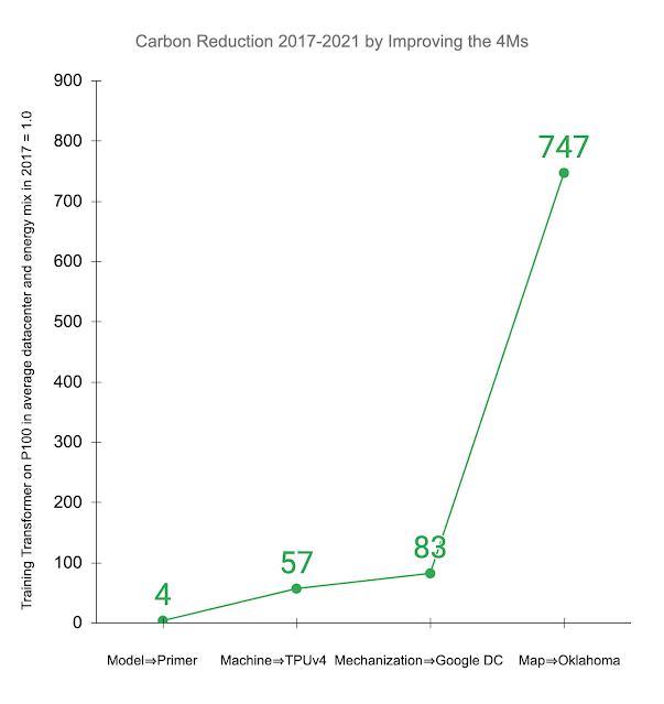
Below, we illustrate the impact of improving the 4Ms in practice. Other studies examined training the Transformer model on an Nvidia P100 GPU in an average data center and energy mix consistent with the worldwide average. The recently introduced Primer model reduces the computation needed to achieve the same accuracy by 4x. Using newer-generation ML hardware, like TPUv4, provides an additional 14x improvement over the P100, or 57x overall. Efficient cloud data centers gain 1.4x over the average data center, resulting in a total energy reduction of 83x. In addition, using a data center with a low-carbon energy source can reduce the carbon footprint another 9x, resulting in a 747x total reduction in carbon footprint over four years.
Reduction in gross carbon dioxide equivalent emissions (CO2e) from applying the 4M best practices to the Transformer model trained on P100 GPUs in an average data center in 2017, as done in other studies. Displayed values are the cumulative improvement successively addressing each of the 4Ms: updating the model to Primer; upgrading the ML accelerator to TPUv4; using a Google data center with better PUE than average; and training in a Google Oklahoma data center that uses very clean energy. Overall Energy Consumption for ML
Google’s total energy usage increases annually, which is not surprising considering increased use of its services. ML workloads have grown rapidly, as has the computation per training run, but paying attention to the 4Ms — optimized models, ML-specific hardware, efficient data centers — has largely compensated for this increased load. Our data shows that ML training and inference are only 10%–15% of Google’s total energy use for each of the last three years, each year split ⅗ for inference and ⅖ for training.Prior Emission Estimates
Google uses neural architecture search (NAS) to find better ML models. NAS is typically performed once per problem domain/search space combination, and the resulting model can then be reused for thousands of applications — e.g., the Evolved Transformer model found by NAS is open sourced for all to use. As the optimized model found by NAS is often more efficient, the one time cost of NAS is typically more than offset by emission reductions from subsequent use.A study from the University of Massachusetts (UMass) estimated carbon emissions for the Evolved Transformer NAS.
- Without ready access to Google hardware or data centers, the study extrapolated from the available P100 GPUs instead of TPUv2s, and assumed US average data center efficiency instead of highly efficient hyperscale data centers. These assumptions increased the estimate by 5x over the energy used by the actual NAS computation that was performed in Google’s data center.
- In order to accurately estimate the emissions for NAS, it's important to understand the subtleties of how they work. NAS systems use a much smaller proxy task to search for the most efficient models to save time, and then scale up the found models to full size. The UMass study assumed that the search repeated full size model training thousands of times, resulting in emission estimates that are another 18.7x too high.
The overshoot for the NAS was 88x: 5x for energy-efficient hardware in Google data centers and 18.7x for computation using proxies. The actual CO2e for the one-time search were 3,223 kg versus 284,019 kg, 88x less than the published estimate.
Unfortunately, some subsequent papers misinterpreted the NAS estimate as the training cost for the model it discovered, yet emissions for this particular NAS are ~1300x larger than for training the model. These papers estimated that training the Evolved Transformer model takes two million GPU hours, costs millions of dollars, and that its carbon emissions are equivalent to five times the lifetime emissions of a car. In reality, training the Evolved Transformer model on the task examined by the UMass researchers and following the 4M best practices takes 120 TPUv2 hours, costs $40, and emits only 2.4 kg (0.00004 car lifetimes), 120,000x less. This gap is nearly as large as if one overestimated the CO2e to manufacture a car by 100x and then used that number as the CO2e for driving a car.
Outlook
Climate change is important, so we must get the numbers right to ensure that we focus on solving the biggest challenges. Within information technology, we believe these are much more likely the lifecycle costs — i.e., emission estimates that include the embedded carbon emitted from manufacturing all components involved, from chips to data center buildings — of manufacturing computing equipment of all types and sizes1 rather than the operational cost of ML training.Expect more good news if everyone improves the 4Ms. While these numbers may currently vary across companies, these simple measures can be followed across the industry:
- Data center providers should publish data center efficiency and the cleanliness of the energy supply per location so that customers can understand and reduce their energy consumption and carbon footprint.
- ML practitioners should train models using the best processors in the greenest data centers, which today are often in the Cloud.
- ML researchers should continue to develop more efficient ML models, for example, by leveraging sparsity or by integrating retrieval to shrink the model. They should also publish energy consumption and carbon footprint, both to foster competition beyond model quality and to ensure accurate accounting of their work, which is difficult to do accurately post-hoc.
If the 4Ms become widely recognized, we predict a virtuous circle that will bend the curve so that the global carbon footprint of ML training is actually shrinking, not increasing.
Acknowledgements
Let me thank my co-authors who stayed with this long and winding investigation into a topic that was new to most of us: Jeff Dean, Joseph Gonzalez, Urs Hölzle, Quoc Le, Chen Liang, Lluis-Miquel Munguia, Daniel Rothchild, David So, and Maud Texier. We also had a great deal of help from others along the way for an earlier study that eventually led to this version of the paper. Emma Strubell made several suggestions for the prior paper, including the recommendation to examine the recent giant NLP models. Christopher Berner, Ilya Sutskever, OpenAI, and Microsoft shared information about GPT-3. Dmitry Lepikhin and Zongwei Zhou did a great deal of work to measure the performance and power of GPUs and TPUs in Google data centers. Hallie Cramer, Anna Escuer, Elke Michlmayr, Kelli Wright, and Nick Zakrasek helped with the data and policies for energy and CO2e emissions at Google.
1Worldwide IT manufacturing for 2021 included 1700M cell phones, 340M PCs, and 12M data center servers. ↩Source: Google AI Blog
How to get started in cloud computing
Posted by Google Cloud training & certifications team
Validated cloud skills are in demand. With Google Cloud certifications, employers know that certified individuals have proven knowledge of various professional roles within the cloud industry. Google Cloud certifications have also been recognized as some of the highest-paying IT certifications for the past several years. This year, the Google Cloud Certified Professional Data Engineer topped the list with an average salary of $171,749, while the Google Cloud Certified Professional Cloud Architect came in second place, with an average salary of $169,029.
You may be wondering what sort of background you need to take advantage of these opportunities: What sort of classes should you take? How exactly do you get started in the cloud without experience? Here are some tips to start learning about Google Cloud and build your cloud computing skills.
Get hands-on experience with cloud computing
Google Cloud training offers a wide range of learning paths featuring comprehensive courses and hands-on labs, so you get to practice with the real Google Cloud console. For instance, If you wanted to take classes to prepare for the Professional Data Engineer certification mentioned above, there is a complete learning path featuring four courses and 31 hands-on labs to help familiarize you with relevant topics like BigQuery, machine learning, IoT, TensorFlow, and more.There are nine learning paths providing you with a launch pad to all major pillars of cloud computing, from networking, cloud security, database management, and hybrid cloud infrastructure. Each broader learning path contains specific learning paths to help you specifically train for job roles like Machine Learning Engineer. Visit the Google Cloud training page to find the right path for you.
Learn live from cloud experts
Google Cloud regularly hosts a half-day live training event called Cloud OnBoard which features hands-on learning led by experts. All sessions are also available to watch on-demand after the event.
If you’re a developer new to cloud computing, we recommend you start with Google Cloud Fundamentals, an entry-level course to learn about the basics of Google Cloud. Experts guide you through hands-on labs where you can practice using the Google Console, Google Cloud Shell, and more.
You’ll be introduced to core components of Google Cloud and given an overview of how its tools impact the entire cloud computing landscape. The curriculum covers Compute Engine and how to create VM instances from scratch and from existing templates, how to connect them together, and end with projects that can talk to each other safely and securely. You will also learn about the different storage and database options available on Google Cloud.
Other Cloud OnBoard event topics include cloud architecture, Kubernetes, data analytics, and cloud application development.
Explore Google Cloud infrastructure
Cloud infrastructure is the backbone of the internet. Understanding cloud infrastructure is a good starting point to start digging deeper into cloud concepts because it will give you a taste of the various aspects of cloud computing to figure out what you like best, whether it’s networking, security, or application development.
Build your foundational Google Cloud knowledge with our on-demand infrastructure training in the cloud infrastructure learning path. This learning path will provide you with practical experience through expert-guided labs which dive into Cloud Storage and other key application services like Google Cloud’s operations suite and Cloud Functions.
Show off your skills
Once you have a strong grasp on Google Cloud basics, you can start earning skill badges to demonstrate your experience.
Skill badges are digital credentials that recognize your ability to solve real-world problems with your cloud knowledge. You can share them on your resume or social profile so your professional network sees your technical skills. This can be useful for recruiters or employers as you transition to cloud computing work.Skill badges also enable you to get in-depth, hands-on experience with different Google Cloud offerings on the way to earning the credential.
You can also use them to start preparing for Google Cloud certifications which are more intensive and show employers that you are a cloud expert. Most Google Cloud certifications recommend having at least 6 months or up to several years of industry experience depending on the material.
Ready to get started in the cloud? Visit the Google Cloud training page to see all your options from in-person classes, online courses, special events, and more.
Source: Google Developers Blog
An ML-Based Framework for COVID-19 Epidemiology
Over the past 20 months, the COVID-19 pandemic has had a profound impact on daily life, presented logistical challenges for businesses planning for supply and demand, and created difficulties for governments and organizations working to support communities with timely public health responses. While there have been well-studied epidemiology models that can help predict COVID-19 cases and deaths to help with these challenges, this pandemic has generated an unprecedented amount of real-time publicly-available data, which makes it possible to use more advanced machine learning techniques in order to improve results.
In "A prospective evaluation of AI-augmented epidemiology to forecast COVID-19 in the USA and Japan", accepted to npj Digital Medicine, we continued our previous work [1, 2, 3, 4] and proposed a framework designed to simulate the effect of certain policy changes on COVID-19 deaths and cases, such as school closings or a state-of-emergency at a US-state, US-county, and Japan-prefecture level, using only publicly-available data. We conducted a 2-month prospective assessment of our public forecasts, during which our US model tied or outperformed all other 33 models on COVID19 Forecast Hub. We also released a fairness analysis of the performance on protected sub-groups in the US and Japan. Like other Google initiatives to help with COVID-19 [1, 2, 3], we are releasing daily forecasts based on this work to the public for free, on the web [us, ja] and through BigQuery.
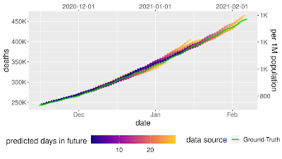
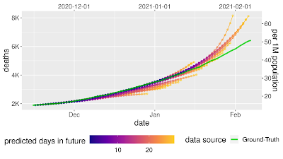
Prospective forecasts for the USA and Japan models. Ground truth cumulative deaths counts (green lines) are shown alongside the forecasts for each day. Each daily forecast contains a predicted increase in deaths for each day during the prediction window of 4 weeks (shown as colored dots, where shading shifting to yellow indicates days further from the date of prediction in the forecasting horizon, up to 4 weeks). Predictions of deaths are shown for the USA (above) and Japan (below). The Model
Models for infectious diseases have been studied by epidemiologists for decades. Compartmental models are the most common, as they are simple, interpretable, and can fit different disease phases effectively. In compartmental models, individuals are separated into mutually exclusive groups, or compartments, based on their disease status (such as susceptible, exposed, or recovered), and the rates of change between these compartments are modeled to fit the past data. A population is assigned to compartments representing disease states, with people flowing between states as their disease status changes.In this work, we propose a few extensions to the Susceptible-Exposed-Infectious-Removed (SEIR) type compartmental model. For example, susceptible people becoming exposed causes the susceptible compartment to decrease and the exposed compartment to increase, with a rate that depends on disease spreading characteristics. Observed data for COVID-19 associated outcomes, such as confirmed cases, hospitalizations and deaths, are used for training of compartmental models.
Visual explanation of "compartmental” models in epidemiology. People "flow" between compartments. Real-world events, like policy changes and more ICU beds, change the rate of flow between compartments. Our framework proposes a number of novel technical innovations:
- Learned transition rates: Instead of using static rates for transitions between compartments across all locations and times, we use machine-learned rates to map them. This allows us to take advantage of the vast amount of available data with informative signals, such as Google's COVID-19 Community Mobility Reports, healthcare supply, demographics, and econometrics features.
- Explainability: Our framework provides explainability for decision makers, offering insights on disease propagation trends via its compartmental structure, and suggesting which factors may be most important for driving compartmental transitions.
- Expanded compartments: We add hospitalization, ICU, ventilator, and vaccine compartments and demonstrate efficient training despite data sparsity.
- Information sharing across locations: As opposed to fitting to an individual location, we have a single model for all locations in a country (e.g., >3000 US counties) with distinct dynamics and characteristics, and we show the benefit of transferring information across locations.
- Seq2seq modeling: We use a sequence-to-sequence model with a novel partial teacher forcing approach that minimizes amplified growth of errors into the future.
Forecast Accuracy
Each day, we train models to predict COVID-19 associated outcomes (primarily deaths and cases) 28 days into the future. We report the mean absolute percentage error (MAPE) for both a country-wide score and a location-level score, with both cumulative values and weekly incremental values for COVID-19 associated outcomes.We compare our framework with alternatives for the US from the COVID19 Forecast Hub. In MAPE, our models outperform all other 33 models except one — the ensemble forecast that also includes our model’s predictions, where the difference is not statistically significant.
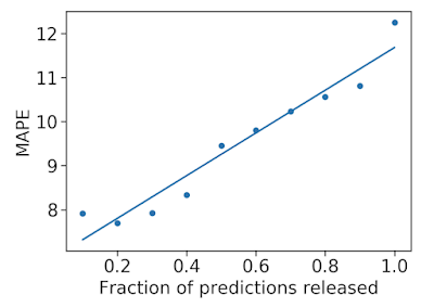
We also used prediction uncertainty to estimate whether a forecast is likely to be accurate. If we reject forecasts that the model considers uncertain, we can improve the accuracy of the forecasts that we do release. This is possible because our model has well-calibrated uncertainty.
Mean average percentage error (MAPE, the lower the better) decreases as we remove uncertain forecasts, increasing accuracy. What-If Tool to Simulate Pandemic Management Policies and Strategies
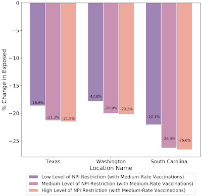
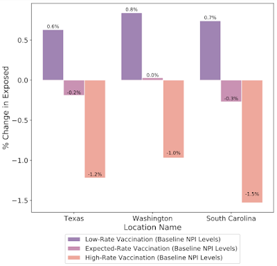
In addition to understanding the most probable scenario given past data, decision makers are interested in how different decisions could affect future outcomes, for example, understanding the impact of school closures, mobility restrictions and different vaccination strategies. Our framework allows counterfactual analysis by replacing the forecasted values for selected variables with their counterfactual counterparts. The results of our simulations reinforce the risk of prematurely relaxing non-pharmaceutical interventions (NPIs) until the rapid disease spreading is reduced. Similarly, the Japan simulations show that maintaining the State of Emergency while having a high vaccination rate greatly reduces infection rates.What-if simulations on the percent change of predicted exposed individuals assuming different non-pharmaceutical interventions (NPIs) for the prediction date of March 1, 2021 in Texas, Washington and South Carolina. Increased NPI restrictions are associated with a larger % reduction in the number of exposed people. What-if simulations on the percent change of predicted exposed individuals assuming different vaccination rates for the prediction date of March 1, 2021 in Texas, Washington and South Carolina. Increased vaccination rate also plays a key role to reduce exposed count in these cases. Fairness Analysis
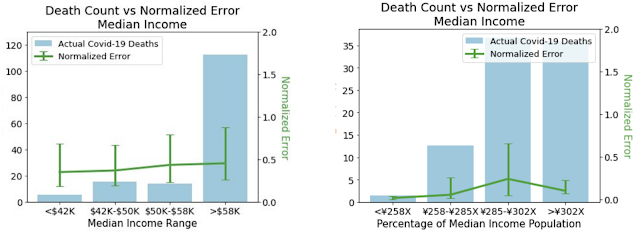
To ensure that our models do not create or reinforce unfairly biased decision making, in alignment with our AI Principles, we performed a fairness analysis separately for forecasts in the US and Japan by quantifying whether the model's accuracy was worse on protected sub-groups. These categories include age, gender, income, and ethnicity in the US, and age, gender, income, and country of origin in Japan. In all cases, we demonstrated no consistent pattern of errors among these groups once we controlled for the number of COVID-19 deaths and cases that occur in each subgroup.Normalized errors by median income. The comparison between the two shows that patterns of errors don't persist once errors are normalized by cases. Left: Normalized errors by median income for the US. Right: Normalized errors by median income for Japan. Real-World Use Cases
In addition to quantitative analyses to measure the performance of our models, we conducted a structured survey in the US and Japan to understand how organisations were using our model forecasts. In total, seven organisations responded with the following results on the applicability of the model.- Organization type: Academia (3), Government (2), Private industry (2)
- Main user job role: Analyst/Scientist (3), Healthcare professional (1), Statistician (2), Managerial (1)
- Location: USA (4), Japan (3)
- Predictions used: Confirmed cases (7), Death (4), Hospitalizations (4), ICU (3), Ventilator (2), Infected (2)
- Model use case: Resource allocation (2), Business planning (2), scenario planning (1), General understanding of COVID spread (1), Confirm existing forecasts (1)
- Frequency of use: Daily (1), Weekly (1), Monthly (1)
- Was the model helpful?: Yes (7)
To share a few examples, in the US, the Harvard Global Health Institute and Brown School of Public Health used the forecasts to help create COVID-19 testing targets that were used by the media to help inform the public. The US Department of Defense used the forecasts to help determine where to allocate resources, and to help take specific events into account. In Japan, the model was used to make business decisions. One large, multi-prefecture company with stores in more than 20 prefectures used the forecasts to better plan their sales forecasting, and to adjust store hours.
Limitations and next steps
Our approach has a few limitations. First, it is limited by available data, and we are only able to release daily forecasts as long as there is reliable, high-quality public data. For instance, public transportation usage could be very useful but that information is not publicly available. Second, there are limitations due to the model capacity of compartmental models as they cannot model very complex dynamics of Covid-19 disease propagation. Third, the distribution of case counts and deaths are very different between the US and Japan. For example, most of Japan's COVID-19 cases and deaths have been concentrated in a few of its 47 prefectures, with the others experiencing low values. This means that our per-prefecture models, which are trained to perform well across all Japanese prefectures, often have to strike a delicate balance between avoiding overfitting to noise while getting supervision from these relatively COVID-19-free prefectures.We have updated our models to take into account large changes in disease dynamics, such as the increasing number of vaccinations. We are also expanding to new engagements with city governments, hospitals, and private organizations. We hope that our public releases continue to help public and policy-makers address the challenges of the ongoing pandemic, and we hope that our method will be useful to epidemiologists and public health officials in this and future health crises.
Acknowledgements
This paper was the result of hard work from a variety of teams within Google and collaborators around the globe. We'd especially like to thank our paper co-authors from the School of Medicine at Keio University, Graduate School of Public Health at St Luke’s International University, and Graduate School of Medicine at The University of Tokyo.Source: Google AI Blog
An easier way to move your App Engine apps to Cloud Run
Posted by Wesley Chun (@wescpy), Developer Advocate, Google Cloud
An easier yet still optional migration
In the previous episode of the Serverless Migration Station video series, developers learned how to containerize their App Engine code for Cloud Run using Docker. While Docker has gained popularity over the past decade, not everyone has containers integrated into their daily development workflow, and some prefer "containerless" solutions but know that containers can be beneficial. Well today's video is just for you, showing how you can still get your apps onto Cloud Run, even If you don't have much experience with Docker, containers, nor
Dockerfiles.App Engine isn't going away as Google has expressed long-term support for legacy runtimes on the platform, so those who prefer source-based deployments can stay where they are so this is an optional migration. Moving to Cloud Run is for those who want to explicitly move to containerization.
Migrating to Cloud Run with Cloud Buildpacks video
So how can apps be containerized without Docker? The answer is buildpacks, an open-source technology that makes it fast and easy for you to create secure, production-ready container images from source code, without a
Dockerfile. Google Cloud Buildpacks adheres to the buildpacks open specification and allows users to create images that run on all GCP container platforms: Cloud Run (fully-managed), Anthos, and Google Kubernetes Engine (GKE). If you want to containerize your apps while staying focused on building your solutions and not how to create or maintainDockerfiles, Cloud Buildpacks is for you.In the last video, we showed developers how to containerize a Python 2 Cloud NDB app as well as a Python 3 Cloud Datastore app. We targeted those specific implementations because Python 2 users are more likely to be using App Engine's
ndbor Cloud NDB to connect with their app's Datastore while Python 3 developers are most likely using Cloud Datastore. Cloud Buildpacks do not support Python 2, so today we're targeting a slightly different audience: Python 2 developers who have migrated from App Engine ndb to Cloud NDB and who have ported their apps to modern Python 3 but now want to containerize them for Cloud Run.Developers familiar with App Engine know that a default HTTP server is provided by default and started automatically, however if special launch instructions are needed, users can add an
entrypointdirective in theirapp.yamlfiles, as illustrated below. When those App Engine apps are containerized for Cloud Run, developers must bundle their own server and provide startup instructions, the purpose of theENTRYPOINTdirective in theDockerfile, also shown below.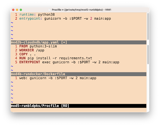
Starting your web server with App Engine (
app.yaml) and Cloud Run with Docker (Dockerfile) or Buildpacks (Procfile)In this migration, there is no
Dockerfile. While Cloud Buildpacks does the heavy-lifting, determining how to package your app into a container, it still needs to be told how to start your service. This is exactly what aProcfileis for, represented by the last file in the image above. As specified, your web server will be launched in the same way as inapp.yamland theDockerfileabove; these config files are deliberately juxtaposed to expose their similarities.Other than this swapping of configuration files and the expected lack of a
.dockerignorefile, the Python 3 Cloud NDB app containerized for Cloud Run is nearly identical to the Python 3 Cloud NDB App Engine app we started with. Cloud Run's build-and-deploy command (gcloud run deploy) will use aDockerfileif present but otherwise selects Cloud Buildpacks to build and deploy the container image. The user experience is the same, only without the time and challenges required to maintain and debug aDockerfile.Get started now
If you're considering containerizing your App Engine apps without having to know much about containers or Docker, we recommend you try this migration on a sample app like ours before considering it for yours. A corresponding codelab leading you step-by-step through this exercise is provided in addition to the video which you can use for guidance.
All migration modules, their videos (when available), codelab tutorials, and source code, can be found in the migration repo. While our content initially focuses on Python users, we hope to one day also cover other legacy runtimes so stay tuned. Containerization may seem foreboding, but the goal is for Cloud Buildpacks and migration resources like this to aid you in your quest to modernize your serverless apps!
Source: Google Developers Blog
Containerizing Google App Engine apps for Cloud Run
Posted by Wesley Chun (@wescpy), Developer Advocate, Google Cloud
An optional migration
Serverless Migration Station is a video mini-series from Serverless Expeditions focused on helping developers modernize their applications running on a serverless compute platform from Google Cloud. Previous episodes demonstrated how to migrate away from the older, legacy App Engine (standard environment) services to newer Google Cloud standalone equivalents like Cloud Datastore. Today's product crossover episode differs slightly from that by migrating away from App Engine altogether, containerizing those apps for Cloud Run.
There's little question the industry has been moving towards containerization as an application deployment mechanism over the past decade. However, Docker and use of containers weren't available to early App Engine developers until its flexible environment became available years later. Fast forward to today where developers have many more options to choose from, from an increasingly open Google Cloud. Google has expressed long-term support for App Engine, and users do not need to containerize their apps, so this is an optional migration. It is primarily for those who have decided to add containerization to their application deployment strategy and want to explicitly migrate to Cloud Run.
If you're thinking about app containerization, the video covers some of the key reasons why you would consider it: you're not subject to traditional serverless restrictions like development language or use of binaries (flexibility); if your code, dependencies, and container build & deploy steps haven't changed, you can recreate the same image with confidence (reproducibility); your application can be deployed elsewhere or be rolled back to a previous working image if necessary (reusable); and you have plenty more options on where to host your app (portability).
Migration and containerization
Legacy App Engine services are available through a set of proprietary, bundled APIs. As you can surmise, those services are not available on Cloud Run. So if you want to containerize your app for Cloud Run, it must be "ready to go," meaning it has migrated to either Google Cloud standalone equivalents or other third-party alternatives. For example, in a recent episode, we demonstrated how to migrate from App Engine ndb to Cloud NDB for Datastore access.
While we've recently begun to produce videos for such migrations, developers can already access code samples and codelab tutorials leading them through a variety of migrations. In today's video, we have both Python 2 and 3 sample apps that have divested from legacy services, thus ready to containerize for Cloud Run. Python 2 App Engine apps accessing Datastore are most likely to be using Cloud NDB whereas it would be Cloud Datastore for Python 3 users, so this is the starting point for this migration.
Because we're "only" switching execution platforms, there are no changes at all to the application code itself. This entire migration is completely based on changing the apps' configurations from App Engine to Cloud Run. In particular, App Engine artifacts such as
app.yaml,appengine_config.py, and thelibfolder are not used in Cloud Run and will be removed. ADockerfilewill be implemented to build your container. Apps with more complex configurations in theirapp.yamlfiles will likely need an equivalentservice.yamlfile for Cloud Run — if so, you'll find this app.yaml to service.yaml conversion tool handy. Following best practices means there'll also be a.dockerignorefile.App Engine and Cloud Functions are sourced-based where Google Cloud automatically provides a default HTTP server like
gunicorn. Cloud Run is a bit more "DIY" because users have to provide a container image, meaning bundling our own server. In this case, we'll pickgunicornexplicitly, adding it to the top of the existingrequirements.txtrequired packages file(s), as you can see in the screenshot below. Also illustrated is theDockerfilewheregunicornis started to serve your app as the final step. The only differences for the Python 2 equivalentDockerfileare: a) require the Cloud NDB package (google-cloud-ndb) instead of Cloud Datastore, and b) start with a Python 2 base image.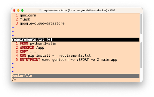
The Python 3
requirements.txtandDockerfileNext steps
To walk developers through migrations, we always "START" with a working app then make the necessary updates that culminate in a working "FINISH" app. For this migration, the Python 2 sample app STARTs with the Module 2a code and FINISHes with the Module 4a code. Similarly, the Python 3 app STARTs with the Module 3b code and FINISHes with the Module 4b code. This way, if something goes wrong during your migration, you can always rollback to START, or compare your solution with our FINISH. If you are considering this migration for your own applications, we recommend you try it on a sample app like ours before considering it for yours. A corresponding codelab leading you step-by-step through this exercise is provided in addition to the video which you can use for guidance.
All migration modules, their videos (when published), codelab tutorials, START and FINISH code, etc., can be found in the migration repo. We hope to also one day cover other legacy runtimes like Java 8 so stay tuned. We'll continue with our journey from App Engine to Cloud Run ahead in Module 5 but will do so without explicit knowledge of containers, Docker, or
Dockerfiles. Modernizing your development workflow to using containers and best practices like crafting a CI/CD pipeline isn't always straightforward; we hope content like this helps you progress in that direction!Source: Google Developers Blog
13 Most Common Google Cloud Reference Architectures
Posted by Priyanka Vergadia, Developer Advocate
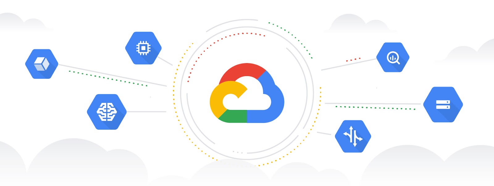
Google Cloud is a cloud computing platform that can be used to build and deploy applications. It allows you to take advantage of the flexibility of development while scaling the infrastructure as needed.
I'm often asked by developers to provide a list of Google Cloud architectures that help to get started on the cloud journey. Last month, I decided to start a mini-series on Twitter called “#13DaysOfGCP" where I shared the most common use cases on Google Cloud. I have compiled the list of all 13 architectures in this post. Some of the topics covered are hybrid cloud, mobile app backends, microservices, serverless, CICD and more. If you were not able to catch it, or if you missed a few days, here we bring to you the summary!

#1: How to set up hybrid architecture in Google Cloud and on-premises

#2: How to mask sensitive data in chatbots using Data loss prevention (DLP) API?

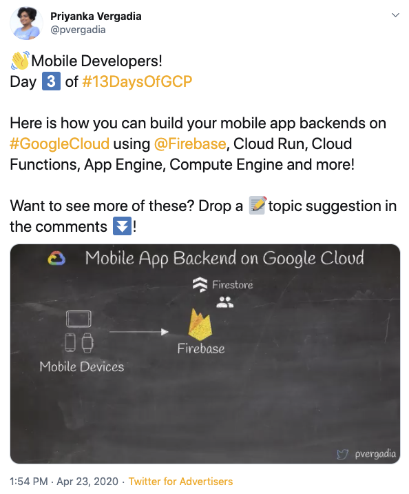
#3: How to build mobile app backends on Google Cloud?
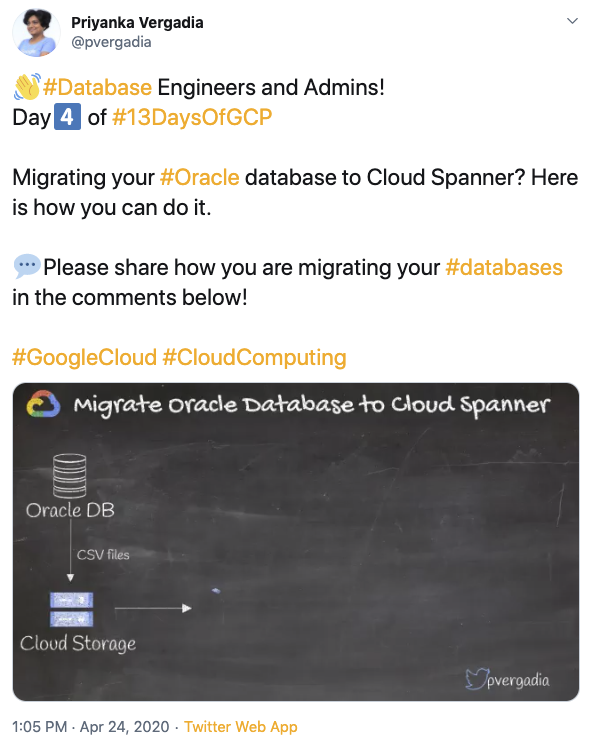
#4: How to migrate Oracle Database to Spanner?
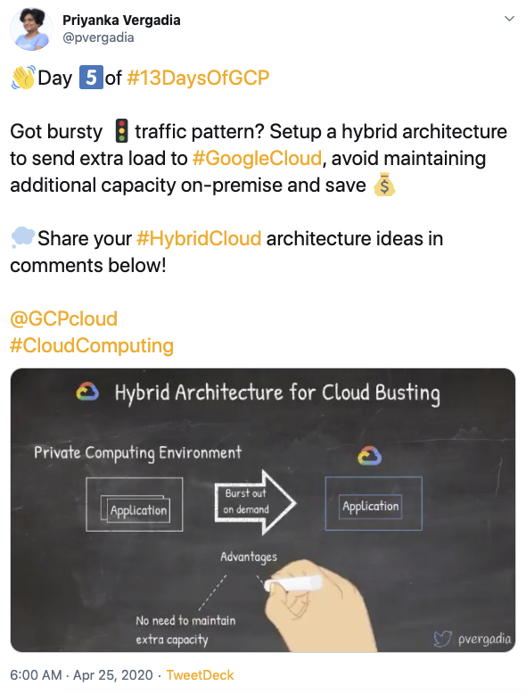
#5: How to set up hybrid architecture for cloud bursting?
#6: How to build a data lake in Google Cloud?

#7: How to host websites on Google Cloud?

#8: How to set up Continuous Integration and Continuous Delivery (CICD) pipeline on Google Cloud?

#9: How to build serverless microservices in Google Cloud?

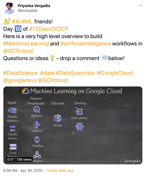
#10: Machine Learning on Google Cloud
#11: Serverless image, video or text processing in Google Cloud

#12: Internet of Things (IoT) on Google Cloud

#13: How to set up BeyondCorp zero trust security model?

Wrap up with a puzzle

We hope you enjoy this list of the most common reference architectures. Please let us know your thoughts in the comments below!
Source: Google Developers Blog
Extracting Structured Data from Templatic Documents
Templatic documents, such as receipts, bills, insurance quotes, and others, are extremely common and critical in a diverse range of business workflows. Currently, processing these documents is largely a manual effort, and automated systems that do exist are based on brittle and error-prone heuristics. Consider a document type like invoices, which can be laid out in thousands of different ways — invoices from different companies, or even different departments within the same company, may have slightly different formatting. However, there is a common understanding of the structured information that an invoice should contain, such as an invoice number, an invoice date, the amount due, the pay-by date, and the list of items for which the invoice was sent. A system that can automatically extract all this data has the potential to dramatically improve the efficiency of many business workflows by avoiding error-prone, manual work.
In “Representation Learning for Information Extraction from Form-like Documents”, accepted to ACL 2020, we present an approach to automatically extract structured data from templatic documents. In contrast to previous work on extraction from plain-text documents, we propose an approach that uses knowledge of target field types to identify candidate fields. These are then scored using a neural network that learns a dense representation of each candidate using the words in its neighborhood. Experiments on two corpora (invoices and receipts) show that we’re able to generalize well to unseen layouts.
Why Is This Hard?
The challenge in this information extraction problem arises because it straddles the natural language processing (NLP) and computer vision worlds. Unlike classic NLP tasks, such documents do not contain “natural language” as might be found in regular sentences and paragraphs, but instead resemble forms. Data is often presented in tables, but in addition many documents have multiple pages, frequently with a varying number of sections, and have a variety of layout and formatting clues to organize the information. An understanding of the two-dimensional layout of text on the page is key to understanding such documents. On the other hand, treating this purely as an image segmentation problem makes it difficult to take advantage of the semantics of the text.
Solution Overview
Our approach to this problem allows developers to train and deploy an extraction system for a given domain (like invoices) using two inputs — a target schema (i.e., a list of fields to extract and their corresponding types) and a small collection of documents labeled with the ground truth for use as a training set. Supported field types include basics, such as dates, integers, alphanumeric codes, currency amounts, phone-numbers, and URLs. We also take advantage of entity types commonly detected by the Google Knowledge Graph, such as addresses, names of companies, etc.
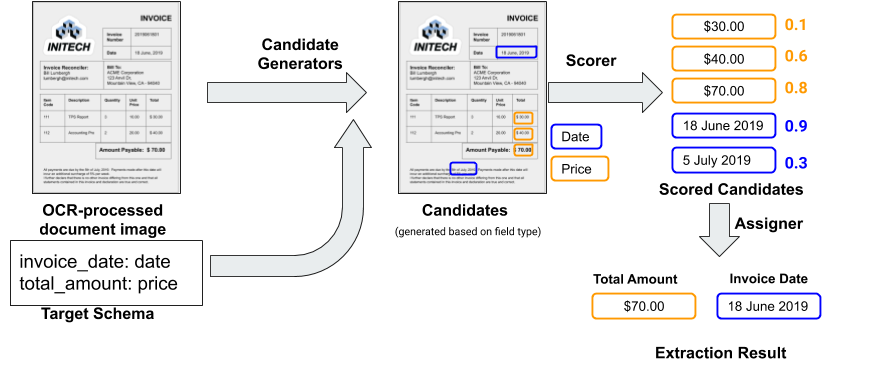
The input document is first run through an Optical Character Recognition (OCR) service to extract the text and layout information, which allows this to work with native digital documents, such as PDFs, and document images (e.g., scanned documents). We then run a candidate generator that identifies spans of text in the OCR output that might correspond to an instance of a given field. The candidate generator utilizes pre-existing libraries associated with each field type (date, number, phone-number, etc.), which avoids the need to write new code for each candidate generator. Each of these candidates is then scored using a trained neural network (the “scorer”, described below) to estimate the likelihood that it is indeed a value one might extract for that field. Finally, an assigner module matches the scored candidates to the target fields. By default, the assigner simply chooses the highest scoring candidate for the field, but additional domain-specific constraints can be incorporated, such as requiring that the invoice date field is chronologically before the payment date field.
Scorer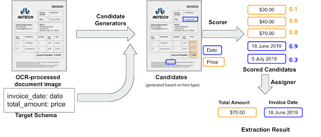
The processing steps in the extraction system using a toy schema with two fields on an input invoice document. Blue boxes show the candidates for the invoice_date field and gold boxes for the amount_due field.
The scorer is a neural model that is trained as a binary classifier. It takes as input the target field from the schema along with the extraction candidate and produces a prediction score between 0 and 1. The target label for a candidate is determined by whether the candidate matches the ground truth for that document and field. The model learns how to represent each field and each candidate in a vector space in which the nearer a field and candidate are in the vector space, the more likely it is that the candidate is the true extraction value for that field and document.
Candidate Representation
A candidate is represented by the tokens in its neighborhood along with the relative position of the token on the page with respect to the centroid of the bounding box identified for the candidate. Using the invoice_date field as an example, phrases in the neighborhood like “Invoice Date’” or “Inv Date” might indicate to the scorer that this is a likely candidate, while phrases like “Delivery Date” would indicate that this is likely not the invoice_date. We do not include the value of the candidate in its representation in order to avoid overfitting to values that happen to be present in a small training data set — e.g., “2019” for the invoice date, if the training corpus happened to include only invoices from that year.
Model Architecture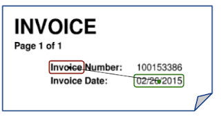
A small snippet of an invoice. The green box shows a candidate for the invoice_date field, and the red box is a token in the neighborhood along with the arrow representing the relative position. Each of the other tokens (‘number’, ‘date’, ‘page’, ‘of’, etc along with the other occurrences of ‘invoice’) are part of the neighborhood for the invoice candidate.
The figure below shows the general structure of the network. In order to construct the candidate encoding (i), each token in the neighborhood is embedded using a word embedding table (a). The relative position of each neighbor (b) is embedded using two fully connected ReLU layers that capture fine-grained non-linearities. The text and position embeddings for each neighbor are concatenated to form a neighbor encoding (d). A self attention mechanism is used to incorporate the neighborhood context for each neighbor (e), which is combined into a neighborhood encoding (f) using max-pooling. The absolute position of the candidate on the page (g) is embedded in a manner similar to the positional embedding for a neighbor, and concatenated with the neighborhood encoding for the candidate encoding (i). The final scoring layer computes the cosine similarity between the field embedding (k) and the candidate encoding (i) and then rescales it to be between 0 and 1.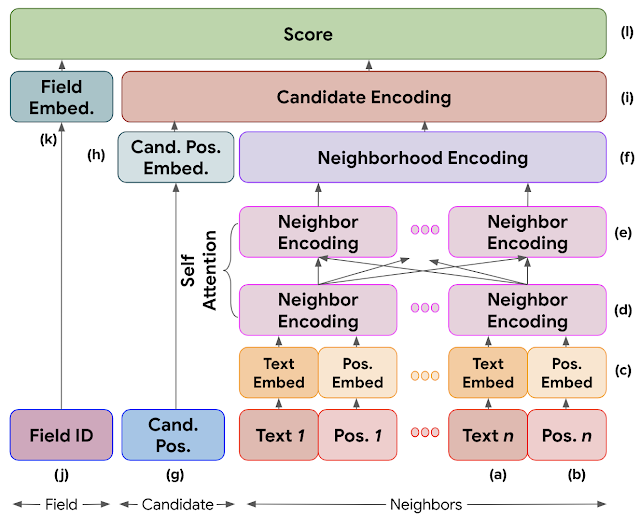
Results
For training and validation, we used an internal dataset of invoices with a large variety of layouts. In order to test the ability of the model to generalize to unseen layouts, we used a test-set of invoices with layouts that were disjoint from the training and validation set. We report the F1 score of the extractions from this system on a few key fields below (higher is better):Field F1 Score amount_due 0.801 delivery_date 0.667 due_date 0.861 invoice_date 0.940 invoice_id 0.949 purchase_order 0.896 total_amount 0.858 total_tax_amount 0.839
As you can see from the table above, the model does well on most fields. However, there’s room for improvement for fields like delivery_date. Additional investigation revealed that this field was present in a very small subset of the examples in our training data. We expect that gathering additional training data will help us improve on it.
What’s next?
Google Cloud recently announced an invoice parsing service as part of the Document AI product. The service uses the methods described above, along with other recent research breakthroughs like BERT, to extract more than a dozen key fields from invoices. You can upload an invoice at the demo page and see this technology in action!
For a given document type we expect to be able to build an extraction system given a modest sized labeled corpus. There are several follow-ons we are currently pursuing, including the improvement of data efficiency and accurately handling nested and repeated fields, and fields for which it is difficult to define a good candidate generator.
Acknowledgements
This work was a collaboration between Google Research and several engineers in Google Cloud. I’d like to thank Navneet Potti, James Wendt, Marc Najork, Qi Zhao, and Ivan Kuznetsov in Google Research as well as Lauro Costa, Evan Huang, Will Lu, Lukas Rutishauser, Mu Wang, and Yang Xu on the Cloud AI team for their support. And finally, our research interns Bodhisattwa Majumder and Beliz Gunel for their tireless experimentation on dozens of ideas.Source: Google AI Blog
Yet More Google Compute Cluster Trace Data
Google’s Borg cluster management system supports our computational fleet, and underpins almost every Google service. For example, the machines that host the Google Doc used for drafting this post are managed by Borg, as are those that run Google’s cloud computing products. That makes the Borg system, as well as its workload, of great interest to researchers and practitioners.
Eight years ago Google published a 29-day cluster trace — a record of every job submission, scheduling decision, and resource usage data for all the jobs in a Google Borg compute cluster, from May 2011. That trace has enabled a wide range of research on advancing the state of the art for cluster schedulers and cloud computing, and has been used to generate hundreds of analyses and studies. But in the years since the 2011 trace was made available, machines and software have evolved, workloads have changed, and the importance of workload variance has become even clearer.
To help researchers explore these changes themselves, we have released a new trace dataset for the month of May 2019 covering eight Google compute clusters. This new dataset is both larger and more extensive than the 2011 one, and now includes:- CPU usage information histograms for each 5 minute period, not just a point sample;
- information about alloc sets (shared resource reservations used by jobs);
- job-parent information for master/worker relationships such as MapReduce jobs.
At this time, we are making the trace data available via Google BigQuery so that sophisticated analyses can be performed without requiring local resources. This site provides access instructions and a detailed description of what the traces contain.
A first analysis of differences between the 2011 and 2019 traces appears in this paper.
We hope this data will facilitate even more research into cluster management. Do let us know if you find it useful, publish papers that use it, develop tools that analyze it, or have suggestions for how to improve it.
Acknowledgements
I’d especially like to thank our intern Muhammad Tirmazi, and my colleagues Nan Deng, Md Ehtesam Haque, Zhijing Gene Qin, Steve Hand and Visiting Researcher Adam Barker for doing the heavy lifting of preparing the new trace set.Source: Google AI Blog
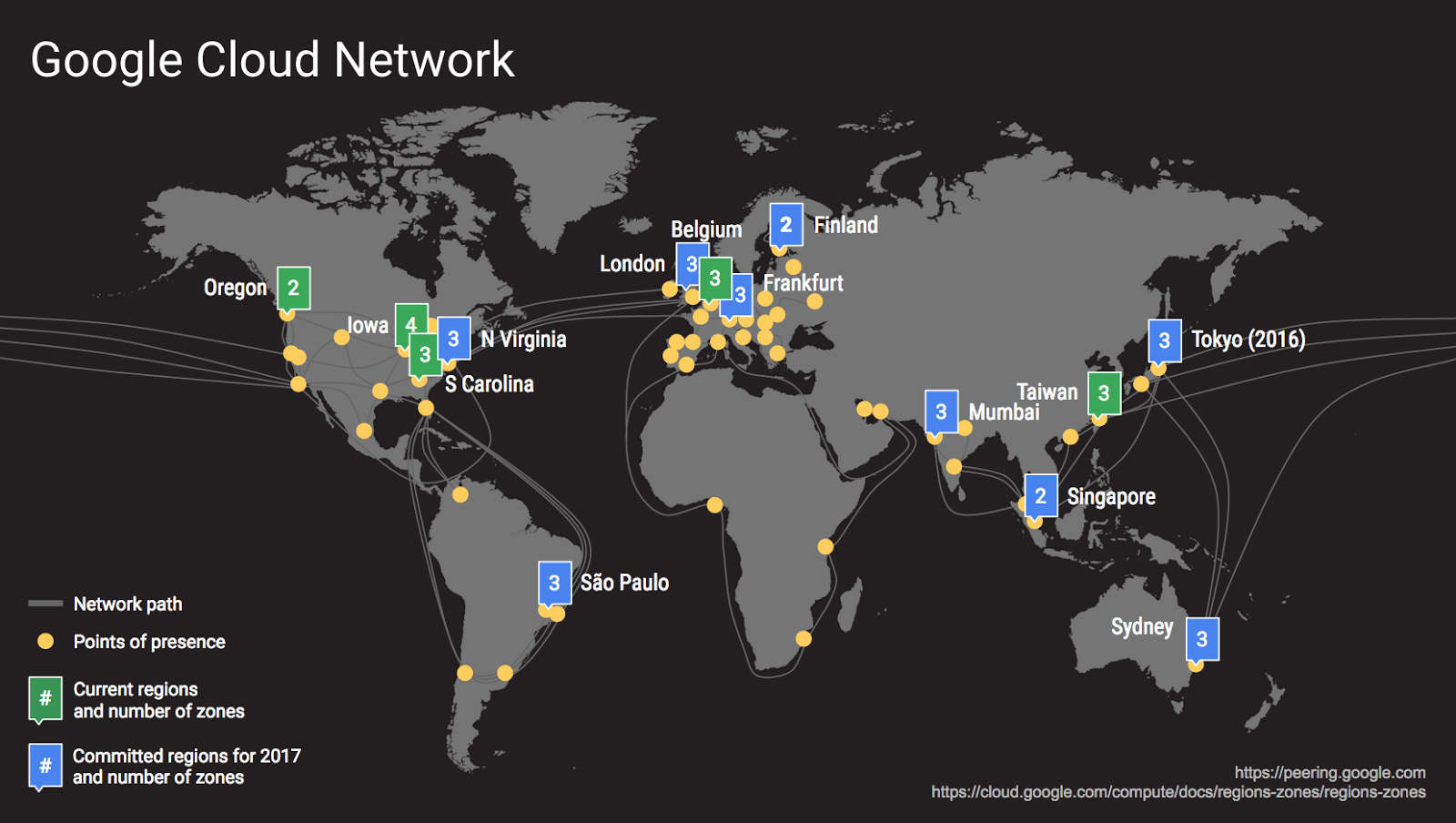
Introducing Google Cloud & India Google Cloud Region
Indian businesses starting today are born in the cloud, while established enterprises are making the move quite rapidly. As digital transformation gains momentum in India, I am excited to share that we are deepening our local investment with the launch of Google Cloud and a Google Cloud Region in Mumbai in 2017.Today, at Horizon in San Francisco, we unveiled Google Cloud, Google’s unique and broad portfolio of products, technologies and services that let our customers operate in a digital world easily and at peak performance. Further, we announced that to offer an even faster experience for Indian developers and enterprise customers, we are bringing a Cloud Region to Mumbai, India. Further, to meet growing demand, we announced the locations of seven new Google Cloud Regions - Singapore, Sydney, Northern Virginia, São Paulo, London, Finland and Frankfurt. Like Mumbai, each of these regions will come online through 2017.Our investment in a local Cloud Region reaffirms our commitment to our customers in India. The local region will help make Google Cloud Platform services even faster for Indian developers and enterprise customers, enhancing differentiators that are already motivating companies to choose us as their partner. As India’s startup community continues to grow, Cloud Platform provides the full stack of services to build, test and deploy their applications.With more than one billion end users, we’ve gained significant traction in India and across the world. Globally, key customers already leveraging the benefits of Google Cloud Platform include SnapChat creator Snap Inc, Pokemon Go creator Niantic Labs and Evernote. In India too, we have seen great customer momentum with thousands of customers including major brands like Wipro, Ashok Leyland, Smartshift by Mahindra & Mahindra, Dainik Bhaskar Group and INshorts.com building on Google Cloud Platform.At Horizon, we further announced G Suite. Previously called Google Apps for Work, G Suite encompasses a set of intelligent apps - Gmail, Docs, Drive, Calendar, Hangouts, and more - designed to bring people together, with real-time collaboration built in from the start.In addition to our focus on Indian customers, we continue to build a robust partner ecosystem to support customers as they move to the cloud. We already have deep partnerships with a multitude of born-in-the-cloud partners including Searce Co-Sourcing, Cloud Cover, PowerUp Cloud and MediaAgility as well as global partners like Wipro, TCS, Tech Mahindra and Cognizant. The opening of the Cloud Region opens up newer opportunities for several new cloud partners who will benefit from building their services on Google Cloud.Posted by Rick Harshman, Asia-Pacific Managing Director, Google CloudSource: Official Google India Blog