Tag Archives: Structured Data

Unsupervised and semi-supervised anomaly detection with data-centric ML

Anomaly detection (AD), the task of distinguishing anomalies from normal data, plays a vital role in many real-world applications, such as detecting faulty products from vision sensors in manufacturing, fraudulent behaviors in financial transactions, or network security threats. Depending on the availability of the type of data — negative (normal) vs. positive (anomalous) and the availability of their labels — the task of AD involves different challenges.
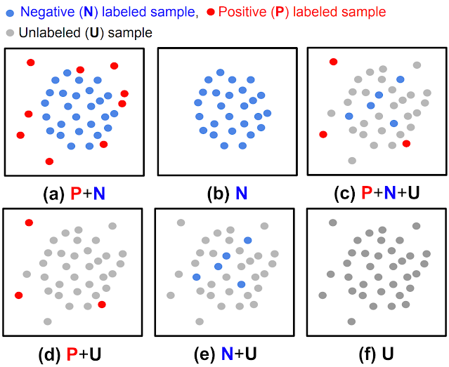
(a) Fully supervised anomaly detection, (b) normal-only anomaly detection, (c, d, e) semi-supervised anomaly detection, (f) unsupervised anomaly detection.

While most previous works were shown to be effective for cases with fully-labeled data (either (a) or (b) in the above figure), such settings are less common in practice because labels are particularly tedious to obtain. In most scenarios users have a limited labeling budget, and sometimes there aren’t even any labeled samples during training. Furthermore, even when labeled data are available, there could be biases in the way samples are labeled, causing distribution differences. Such real-world data challenges limit the achievable accuracy of prior methods in detecting anomalies.

This post covers two of our recent papers on AD, published in Transactions on Machine Learning Research (TMLR), that address the above challenges in unsupervised and semi-supervised settings. Using data-centric approaches, we show state-of-the-art results in both. In “Self-supervised, Refine, Repeat: Improving Unsupervised Anomaly Detection”, we propose a novel unsupervised AD framework that relies on the principles of self-supervised learning without labels and iterative data refinement based on the agreement of one-class classifier (OCC) outputs. In “SPADE: Semi-supervised Anomaly Detection under Distribution Mismatch”, we propose a novel semi-supervised AD framework that yields robust performance even under distribution mismatch with limited labeled samples.


Unsupervised anomaly detection with SRR: Self-supervised, Refine, Repeat

Discovering a decision boundary for a one-class (normal) distribution (i.e., OCC training) is challenging in fully unsupervised settings as unlabeled training data include two classes (normal and abnormal). The challenge gets further exacerbated as the anomaly ratio gets higher for unlabeled data. To construct a robust OCC with unlabeled data, excluding likely-positive (anomalous) samples from the unlabeled data, the process referred to as data refinement, is critical. The refined data, with a lower anomaly ratio, are shown to yield superior anomaly detection models.

SRR first refines data from an unlabeled dataset, then iteratively trains deep representations using refined data while improving the refinement of unlabeled data by excluding likely-positive samples. For data refinement, an ensemble of OCCs is employed, each of which is trained on a disjoint subset of unlabeled training data. If there is consensus among all the OCCs in the ensemble, the data that are predicted to be negative (normal) are included in the refined data. Finally, the refined training data are used to train the final OCC to generate the anomaly predictions.
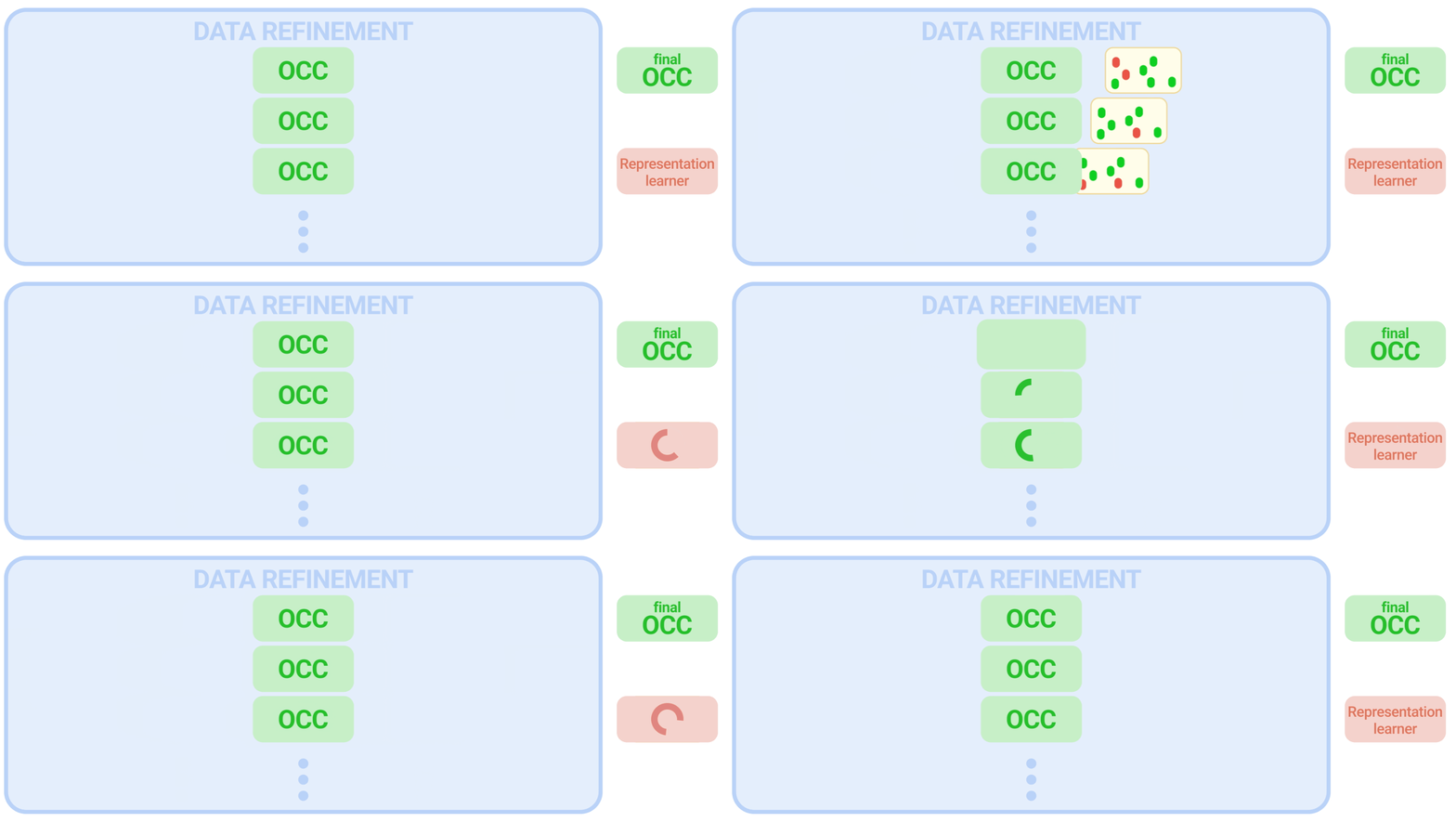
Training SRR with a data refinement module (OCCs ensemble), representation learner, and final OCC. (Green/red dots represent normal/abnormal samples, respectively).

SRR results

We conduct extensive experiments across various datasets from different domains, including semantic AD (CIFAR-10, Dog-vs-Cat), real-world manufacturing visual AD (MVTec), and real-world tabular AD benchmarks such as detecting medical (Thyroid) or network security (KDD 1999) anomalies. We consider methods with both shallow (e.g., OC-SVM) and deep (e.g., GOAD, CutPaste) models. Since the anomaly ratio of real-world data can vary, we evaluate models at different anomaly ratios of unlabeled training data and show that SRR significantly boosts AD performance. For example, SRR improves more than 15.0 average precision (AP) with a 10% anomaly ratio compared to a state-of-the-art one-class deep model on CIFAR-10. Similarly, on MVTec, SRR retains solid performance, dropping less than 1.0 AUC with a 10% anomaly ratio, while the best existing OCC drops more than 6.0 AUC. Lastly, on Thyroid (tabular data), SRR outperforms a state-of-the-art one-class classifier by 22.9 F1 score with a 2.5% anomaly ratio.

Across various domains, SRR (blue line) significantly boosts AD performance with various anomaly ratios in fully unsupervised settings.

SPADE: Semi-supervised Pseudo-labeler Anomaly Detection with Ensembling

Most semi-supervised learning methods (e.g., FixMatch, VIME) assume that the labeled and unlabeled data come from the same distributions. However, in practice, distribution mismatch commonly occurs, with labeled and unlabeled data coming from different distributions. One such case is positive and unlabeled (PU) or negative and unlabeled (NU) settings, where the distributions between labeled (either positive or negative) and unlabeled (both positive and negative) samples are different. Another cause of distribution shift is additional unlabeled data being gathered after labeling. For example, manufacturing processes may keep evolving, causing the corresponding defects to change and the defect types at labeling to differ from the defect types in unlabeled data. In addition, for applications like financial fraud detection and anti-money laundering, new anomalies can appear after the data labeling process, as criminal behavior may adapt. Lastly, labelers are more confident on easy samples when they label them; thus, easy/difficult samples are more likely to be included in the labeled/unlabeled data. For example, with some crowd-sourcing–based labeling, only the samples with some consensus on the labels (as a measure of confidence) are included in the labeled set.
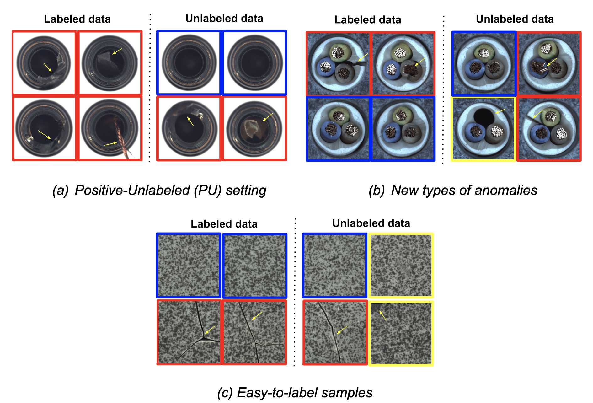
Three common real-world scenarios with distribution mismatches (blue box: normal samples, red box: known/easy anomaly samples, yellow box: new/difficult anomaly samples).

Standard semi-supervised learning methods assume that labeled and unlabeled data come from the same distribution, so are sub-optimal for semi-supervised AD under distribution mismatch. SPADE utilizes an ensemble of OCCs to estimate the pseudo-labels of the unlabeled data — it does this independent of the given positive labeled data, thus reducing the dependency on the labels. This is especially beneficial when there is a distribution mismatch. In addition, SPADE employs partial matching to automatically select the critical hyper-parameters for pseudo-labeling without relying on labeled validation data, a crucial capability given limited labeled data.
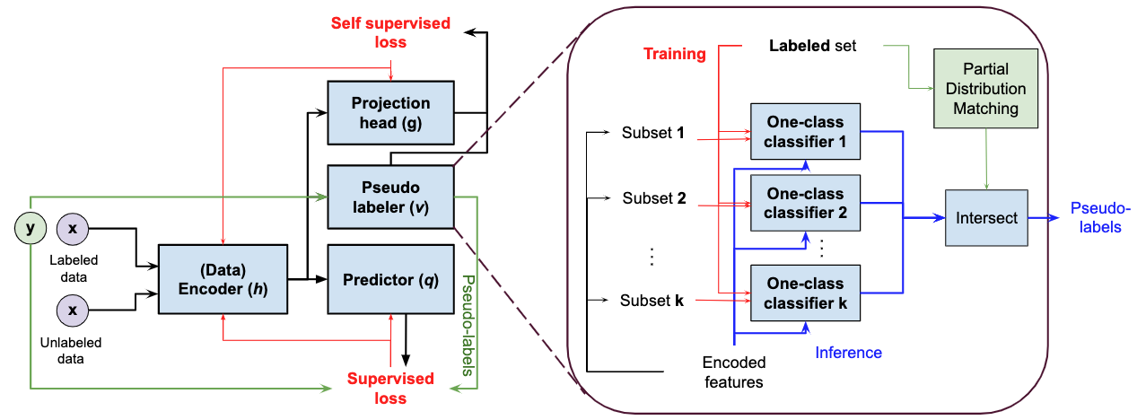
Block diagram of SPADE with zoom in the detailed block diagram of the proposed pseudo-labelers.

SPADE results

We conduct extensive experiments to showcase the benefits of SPADE in various real-world settings of semi-supervised learning with distribution mismatch. We consider multiple AD datasets for image (including MVTec) and tabular (including Covertype, Thyroid) data.

SPADE shows state-of-the-art semi-supervised anomaly detection performance across a wide range of scenarios: (i) new-types of anomalies, (ii) easy-to-label samples, and (iii) positive-unlabeled examples. As shown below, with new-types of anomalies, SPADE outperforms the state-of-the-art alternatives by 5% AUC on average.
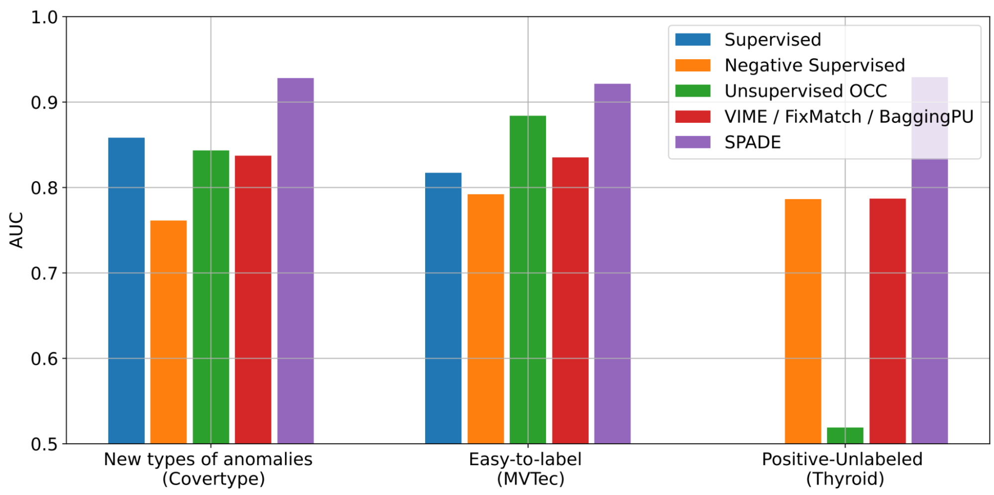
AD performances with three different scenarios across various datasets (Covertype, MVTec, Thyroid) in terms of AUC. Some baselines are only applicable to some scenarios. More results with other baselines and datasets can be found in the paper.

We also evaluate SPADE on real-world financial fraud detection datasets: Kaggle credit card fraud and Xente fraud detection. For these, anomalies evolve (i.e., their distributions change over time) and to identify evolving anomalies, we need to keep labeling for new anomalies and retrain the AD model. However, labeling would be costly and time consuming. Even without additional labeling, SPADE can improve the AD performance using both labeled data and newly-gathered unlabeled data.
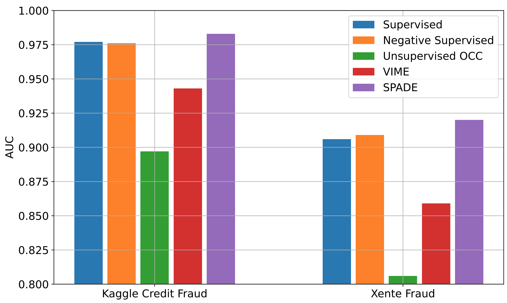
AD performances with time-varying distributions using two real-world fraud detection datasets with 10% labeling ratio. More baselines can be found in the paper.

As shown above, SPADE consistently outperforms alternatives on both datasets, taking advantage of the unlabeled data and showing robustness to evolving distributions.


Conclusions

AD has a wide range of use cases with significant importance in real-world applications, from detecting security threats in financial systems to identifying faulty behaviors of manufacturing machines.

One challenging and costly aspect of building an AD system is that anomalies are rare and not easily detectable by people. To this end, we have proposed SRR, a canonical AD framework to enable high performance AD without the need for manual labels for training. SRR can be flexibly integrated with any OCC, and applied on raw data or on trainable representations.

Semi-supervised AD is another highly-important challenge — in many scenarios, the distributions of labeled and unlabeled samples don’t match. SPADE introduces a robust pseudo-labeling mechanism using an ensemble of OCCs and a judicious way of combining supervised and self-supervised learning. In addition, SPADE introduces an efficient approach to pick critical hyperparameters without a validation set, a crucial component for data-efficient AD.

Overall, we demonstrate that SRR and SPADE consistently outperform the alternatives in various scenarios across multiple types of datasets.


Acknowledgements

We gratefully acknowledge the contributions of Kihyuk Sohn, Chun-Liang Li, Chen-Yu Lee, Kyle Ziegler, Nate Yoder, and Tomas Pfister.

Source: Google AI Blog


EHR-Safe: Generating High-Fidelity and Privacy-Preserving Synthetic Electronic Health Records

Analysis of Electronic Health Records (EHR) has a tremendous potential for enhancing patient care, quantitatively measuring performance of clinical practices, and facilitating clinical research. Statistical estimation and machine learning (ML) models trained on EHR data can be used to predict the probability of various diseases (such as diabetes), track patient wellness, and predict how patients respond to specific drugs. For such models, researchers and practitioners need access to EHR data. However, it can be challenging to leverage EHR data while ensuring data privacy and conforming to patient confidentiality regulations (such as HIPAA).

Conventional methods to anonymize data (e.g., de-identification) are often tedious and costly. Moreover, they can distort important features from the original dataset, decreasing the utility of the data significantly; they can also be susceptible to privacy attacks. Alternatively, an approach based on generating synthetic data can maintain both important dataset features and privacy.

To that end, we propose a novel generative modeling framework in “EHR-Safe: Generating High-Fidelity and Privacy-Preserving Synthetic Electronic Health Records". With the innovative methodology in EHR-Safe, we show that synthetic data can satisfy two key properties: (i) high fidelity (i.e., they are useful for the task of interest, such as having similar downstream performance when a diagnostic model is trained on them), (ii) meet certain privacy measures (i.e., they do not reveal any real patient's identity). Our state-of-the-art results stem from novel approaches for encoding/decoding features, normalizing complex distributions, conditioning adversarial training, and representing missing data.

Generating synthetic data from the original data with EHR-Safe.

Challenges of Generating Realistic Synthetic EHR Data

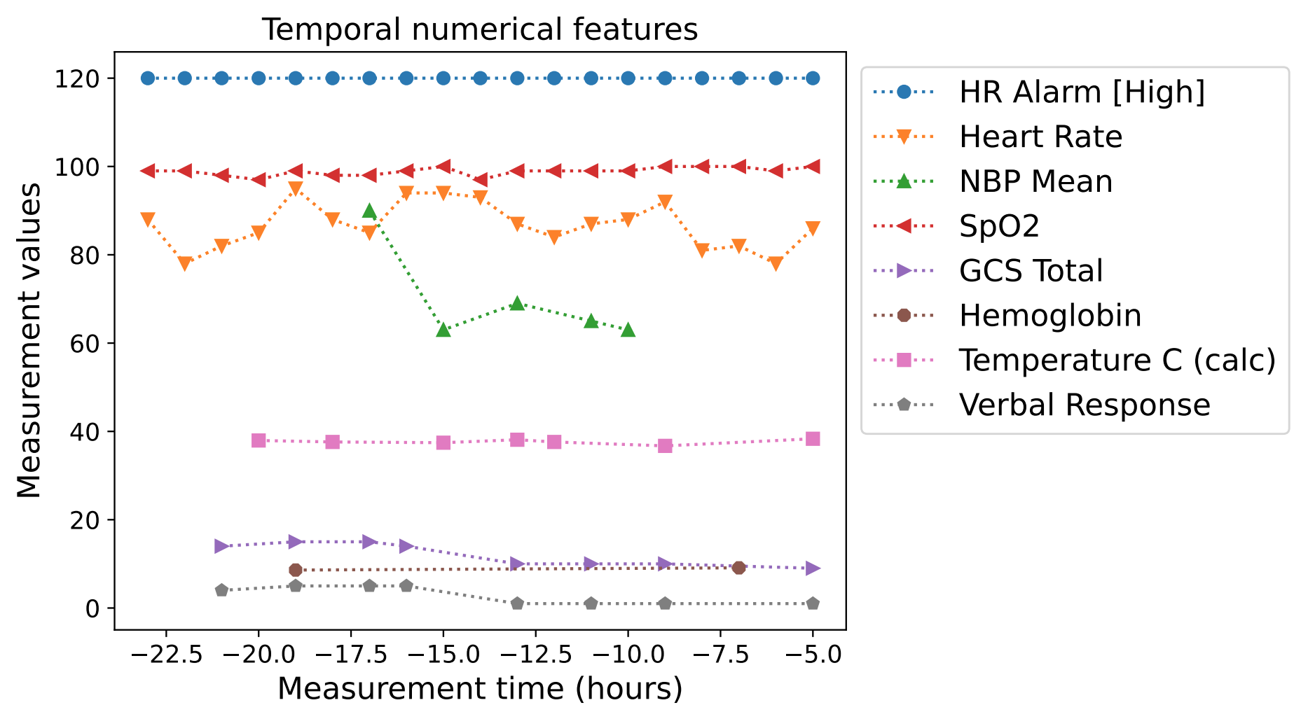
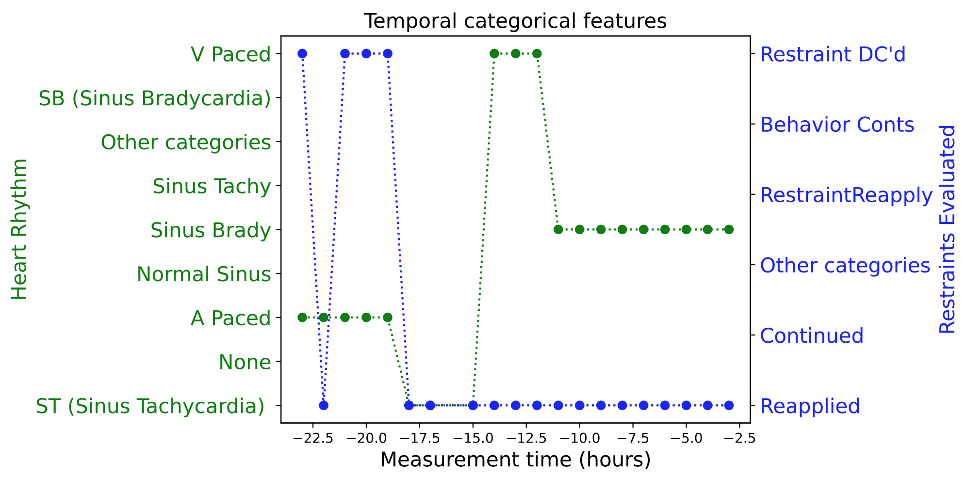
There are multiple fundamental challenges to generating synthetic EHR data. EHR data contain heterogeneous features with different characteristics and distributions. There can be numerical features (e.g., blood pressure) and categorical features with many or two categories (e.g., medical codes, mortality outcome). Some of these may be static (i.e., not varying during the modeling window), while others are time-varying, such as regular or sporadic lab measurements. Distributions might come from different families — categorical distributions can be highly non-uniform (e.g., for under-represented groups) and numerical distributions can be highly skewed (e.g., a small proportion of values being very large while the vast majority are small). Depending on a patient's condition, the number of visits can also vary drastically — some patients visit a clinic only once whereas some visit hundreds of times, leading to a variance in sequence lengths that is typically much higher compared to other time-series data. There can be a high ratio of missing features across different patients and time steps, as not all lab measurements or other input data are collected.

Examples of real EHR data: temporal numerical features (upper) and temporal categorical features (lower).

EHR-Safe: Synthetic EHR Data Generation Framework

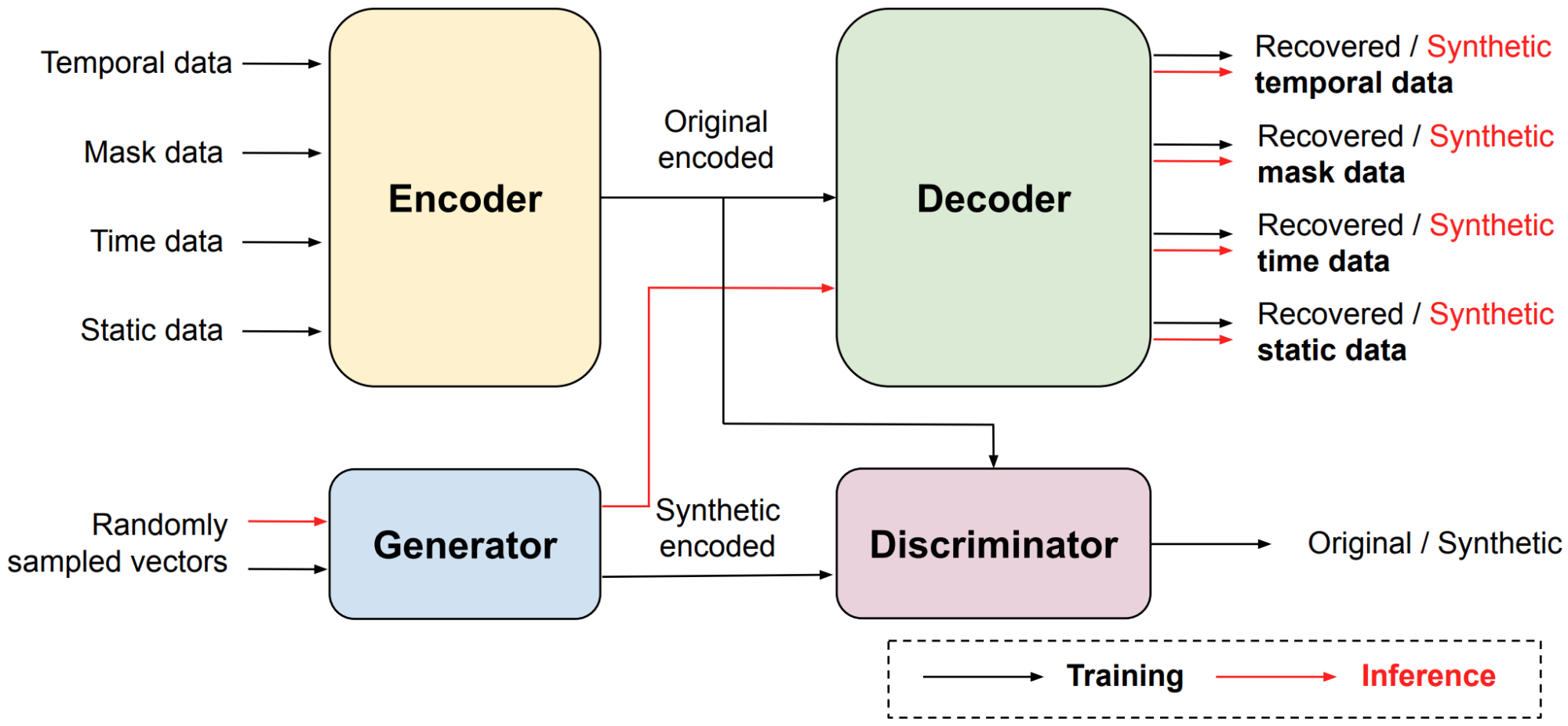
EHR-Safe consists of sequential encoder-decoder architecture and generative adversarial networks (GANs), depicted in the figure below. Because EHR data are heterogeneous (as described above), direct modeling of raw EHR data is challenging for GANs. To circumvent this, we propose utilizing a sequential encoder-decoder architecture, to learn the mapping from the raw EHR data to the latent representations, and vice versa.

Block diagram of EHR-Safe framework.

While learning the mapping, esoteric distributions of numerical and categorical features pose a great challenge. For example, some values or numerical ranges might dominate the distribution, but the capability of modeling rare cases is essential. The proposed feature mapping and stochastic normalization (transforming original feature distributions into uniform distributions without information loss) are key to handling such data by converting to distributions for which the training of encoder-decoder and GAN are more stable (details can be found in the paper). The mapped latent representations, generated by the encoder, are then used for GAN training. After training both the encoder-decoder framework and GANs, EHR-Safe can generate synthetic heterogeneous EHR data from any input, for which we feed randomly sampled vectors. Note that only the trained generator and decoders are used for generating synthetic data.


Datasets

We focus on two real-world EHR datasets to showcase the EHR-Safe framework, MIMIC-III and eICU. Both are inpatient datasets that consist of varying lengths of sequences and include multiple numerical and categorical features with missing components.


Fidelity Results

The fidelity metrics focus on the quality of synthetically generated data by measuring the realisticness of the synthetic data. Higher fidelity implies that it is more difficult to differentiate between synthetic and real data. We evaluate the fidelity of synthetic data in terms of multiple quantitative and qualitative analyses.


Visualization

Having similar coverage and avoiding under-representation of certain data regimes are both important for synthetic data generation. As the below t-SNE analyses show, the coverage of the synthetic data (blue) is very similar with the original data (red). With membership inference metrics (will be introduced in the privacy section), we also verify that EHR-Safe does not just memorize the original train data.

t-SNE analyses on temporal and static data on MIMIC-III (upper) and eICU (lower) datasets.

Statistical Similarity

We provide quantitative comparisons of statistical similarity between original and synthetic data for each feature. Most statistics are well-aligned between original and synthetic data — for example a measure of the KS statistics, i.e,. the maximum difference in the cumulative distribution function (CDF) between the original and the synthetic data, are mostly lower than 0.03. More detailed tables can be found in the paper. The figure below exemplifies the CDF graphs for original vs. synthetic data for three features — overall they seem very close in most cases.

CDF graphs of two features between original and synthetic EHR data. Left: Mean Airway Pressure. Right: Minute Volume Alarm.

Utility

Because one of the most important use cases of synthetic data is enabling ML innovations, we focus on the fidelity metric that measures the ability of models trained on synthetic data to make accurate predictions on real data. We compare such model performance to an equivalent model trained with real data. Similar model performance would indicate that the synthetic data captures the relevant informative content for the task. As one of the important potential use cases of EHR, we focus on the mortality prediction task. We consider four different predictive models: Gradient Boosting Tree Ensemble (GBDT), Random Forest (RF), Logistic Regression (LR), Gated Recurrent Units (GRU).

Mortality prediction performance with the model trained on real vs. synthetic data. Left: MIMIC-III. Right: eICU.

In the figure above we see that in most scenarios, training on synthetic vs. real data are highly similar in terms of Area Under Receiver Operating Characteristics Curve (AUC). On MIMIC-III, the best model (GBDT) on synthetic data is only 2.6% worse than the best model on real data; whereas on eICU, the best model (RF) on synthetic data is only 0.9% worse.


Privacy Results

We consider three different privacy attacks to quantify the robustness of the synthetic data with respect to privacy.

  • Membership inference attack: An adversary predicts whether a known subject was a present in the training data used for training the synthetic data model.
  • Re-identification attack: The adversary explores the probability of some features being re-identified using synthetic data and matching to the training data.
  • Attribute inference attack: The adversary predicts the value of sensitive features using synthetic data.
Privacy risk evaluation across three privacy metrics: membership-inference (top-left), re-identification (top-right), and attribute inference (bottom). The ideal value of privacy risk for membership inference is random guessing (0.5). For re-identification, the ideal case is to replace the synthetic data with disjoint holdout original data.

The figure above summarizes the results along with the ideal achievable value for each metric. We observe that the privacy metrics are very close to the ideal in all cases. The risk of understanding whether a sample of the original data is a member used for training the model is very close to random guessing; it also verifies that EHR-Safe does not just memorize the original train data. For the attribute inference attack, we focus on the prediction task of inferring specific attributes (e.g., gender, religion, and marital status) from other attributes. We compare prediction accuracy when training a classifier with real data against the same classifier trained with synthetic data. Because the EHR-Safe bars are all lower, the results demonstrate that access to synthetic data does not lead to higher prediction performance on specific features as compared to access to the original data.


Comparison to Alternative Methods

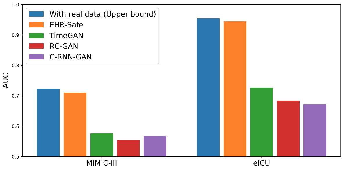
We compare EHR-Safe to alternatives (TimeGAN, RC-GAN, C-RNN-GAN) proposed for time-series synthetic data generation. As shown below, EHR-Safe significantly outperforms each.

Downstream task performance (AUC) in comparison to alternatives.

Conclusions

We propose a novel generative modeling framework, EHR-Safe, that can generate highly realistic synthetic EHR data that are robust to privacy attacks. EHR-Safe is based on generative adversarial networks applied to the encoded raw data. We introduce multiple innovations in the architecture and training mechanisms that are motivated by the key challenges of EHR data. These innovations are key to our results that show almost-identical properties with real data (when desired downstream capabilities are considered) with almost-ideal privacy preservation. An important future direction is generative modeling capability for multimodal data, including text and image, as modern EHR data might contain both.


Acknowledgements

We gratefully acknowledge the contributions of Michel Mizrahi, Nahid Farhady Ghalaty, Thomas Jarvinen, Ashwin S. Ravi, Peter Brune, Fanyu Kong, Dave Anderson, George Lee, Arie Meir, Farhana Bandukwala, Elli Kanal, and Tomas Pfister.

Source: Google AI Blog


schema-dts turns 1.0: Author valid Schema.org JSON-LD in TypeScript

Today, schema-dts turns 1.0 to properly reflect its current maturity. I started the project in November 2018 to improve the developer experience of writing Structured Data.

The project has continued to improve, validating a broader and more complex subset of Schema.org, improving type-checking performance, and eliminating the runtime bundle entirely. Many of these improvements were only fully understood due to feedback and reports from the community. Today, schema-dts receives more than 100k downloads/week on NPM. These users have helped validate and harden the library over the past few years.

Here are some of the highlighted improvement since the last announcement:

0kb Bundle Runtime Size

The library is now entirely type only. Previously, convenience enums were generated in .js files, but improved TypeScript completions mean that this is no longer necessary.

(The first episode, now on your screen)

In this first episode, we cover:

We plan to make these updates regularly, and adjust the format over time as needed. Let us know what you think in the video comments!

An End-to-End AutoML Solution for Tabular Data at KaggleDays


Machine learning (ML) for tabular data (e.g. spreadsheet data) is one of the most active research areas in both ML research and business applications. Solutions to tabular data problems, such as fraud detection and inventory prediction, are critical for many business sectors, including retail, supply chain, finance, manufacturing, marketing and others. Current ML-based solutions to these problems can be achieved by those with significant ML expertise, including manual feature engineering and hyper-parameter tuning, to create a good model. However, the lack of broad availability of these skills limits the efficiency of business improvements through ML.

Google’s AutoML efforts aim to make ML more scalable and accelerate both research and industry applications. Our initial efforts of neural architecture search have enabled breakthroughs in computer vision with NasNet, and evolutionary methods such as AmoebaNet and hardware-aware mobile vision architecture MNasNet further show the benefit of these learning-to-learn methods. Recently, we applied a learning-based approach to tabular data, creating a scalable end-to-end AutoML solution that meets three key criteria:
  • Full automation: Data and computation resources are the only inputs, while a servable TensorFlow model is the output. The whole process requires no human intervention.
  • Extensive coverage: The solution is applicable to the majority of arbitrary tasks in the tabular data domain.
  • High quality: Models generated by AutoML has comparable quality to models manually crafted by top ML experts.
To benchmark our solution, we entered our algorithm in the KaggleDays SF Hackathon, an 8.5 hour competition of 74 teams with up to 3 members per team, as part of the KaggleDays event. The first time that AutoML has competed against Kaggle participants, the competition involved predicting manufacturing defects given information about the material properties and testing results for batches of automotive parts. Despite competing against participants thats were at the Kaggle progression system Master level, including many who were at the GrandMaster level, our team (“Google AutoML”) led for most of the day and ended up finishing second place by a narrow margin, as seen in the final leaderboard.

Our team’s AutoML solution was a multistage TensorFlow pipeline. The first stage is responsible for automatic feature engineering, architecture search, and hyperparameter tuning through search. The promising models from the first stage are fed into the second stage, where cross validation and bootstrap aggregating are applied for better model selection. The best models from the second stage are then combined in the final model.
The workflow for the “Google AutoML” team was quite different from that of other Kaggle competitors. While they were busy with analyzing data and experimenting with various feature engineering ideas, our team spent most of time monitoring jobs and and waiting for them to finish. Our solution for second place on the final leaderboard required 1 hour on 2500 CPUs to finish end-to-end.

After the competition, Kaggle published a public kernel to investigate winning solutions and found that augmenting the top hand-designed models with AutoML models, such as ours, could be a useful way for ML experts to create even better performing systems. As can be seen in the plot below, AutoML has the potential to enhance the efforts of human developers and address a broad range of ML problems.
Potential model quality improvement on final leaderboard if AutoML models were merged with other Kagglers’ models. “Erkut & Mark, Google AutoML”, includes the top winner “Erkut & Mark” and the second place “Google AutoML” models. Erkut Aykutlug and Mark Peng used XGBoost with creative feature engineering whereas AutoML uses both neural network and gradient boosting tree (TFBT) with automatic feature engineering and hyperparameter tuning.
Google Cloud AutoML Tables
The solution we presented at the competitions is the main algorithm in Google Cloud AutoML Tables, which was recently launched (beta) at Google Cloud Next ‘19. The AutoML Tables implementation regularly performs well in benchmark tests against Kaggle competitions as shown in the plot below, demonstrating state-of-the-art performance across the industry.
Third party benchmark of AutoML Tables on multiple Kaggle competitions
We are excited about the potential application of AutoML methods across a wide range of real business problems. Customers have already been leveraging their tabular enterprise data to tackle mission-critical tasks like supply chain management and lead conversion optimization using AutoML Tables, and we are excited to be providing our state-of-the-art models to solve tabular data problems.

Acknowledgements
This project was only possible thanks to Google Brain team members Ming Chen, Da Huang, Yifeng Lu, Quoc V. Le and Vishy Tirumalashetty. We also thank Dawei Jia, Chenyu Zhao and Tin-yun Ho from the Cloud AutoML Tables team for great infrastructure and product landing collaboration. Thanks to Walter Reade, Julia Elliott and Kaggle for organizing such an engaging competition.

Source: Google AI Blog


Google I/O 2019 – What sessions should SEOs and webmasters watch?

Google I/O 2019 is starting tomorrow and will run for 3 days, until Thursday. Google I/O is our yearly developers festival, where product announcements are made, new APIs and frameworks are introduced, and Product Managers present the latest from Google to an audience of 7,000+ developers who fly to California.

However, you don't have to physically attend the event to take advantage of this once-a-year opportunity: many conferences and talks are live streamed on YouTube for anyone to watch. Browse the full schedule of events, including a list of talks that we think will be interesting for webmasters to watch (all talks are in English). All the links shared below will bring you to pages with more details about each talk, and links to watch the sessions will display on the day of each event. All times are Pacific Central time (California time).


This list is only a small part of the agenda that we think is useful to webmasters and SEOs. There are many more sessions that you could find interesting! To learn about those other talks, check out the full list of “web” sessions, design sessions, Cloud sessions, machine learning sessions, and more. Use the filtering function to toggle the sessions on and off.

We hope you can make the time to watch the talks online, and participate in the excitement of I/O ! The videos will also be available on Youtube after the event, in case you can't tune in live.

Posted by Vincent Courson, Search Outreach Specialist

Help Google Search know the best date for your web page

Sometimes, Google shows dates next to listings in its search results. In this post, we’ll answer some commonly-asked questions webmasters have about how these dates are determined and provide some best practices to help improve their accuracy.

How dates are determined

Google shows the date of a page when its automated systems determine that it would be relevant to do so, such as for pages that can be time-sensitive, including news content:

Google determines a date using a variety of factors, including but not limited to: any prominent date listed on the page itself or dates provided by the publisher through structured markup.

Google doesn’t depend on one single factor because all of them can be prone to issues. Publishers may not always provide a clear visible date. Sometimes, structured data may be lacking or may not be adjusted to the correct time zone. That’s why our systems look at several factors to come up with what we consider to be our best estimate of when a page was published or significantly updated.

How to specify a date on a page

To help Google to pick the right date, site owners and publishers should:

  • Show a clear date: Show a visible date prominently on the page.
  • Use structured data: Use the datePublished and dateModified schema with the correct time zone designator for AMP or non-AMP pages. When using structured data, make sure to use the ISO 8601 format for dates.

Guidelines specific to Google News

Google News requires clearly showing both the date and the time that content was published or updated. Structured data alone is not enough, though it is recommended to use in addition to a visible date and time. Date and time should be positioned between the headline and the article text. For more guidance, also see our help page about article dates.

If an article has been substantially changed, it can make sense to give it a fresh date and time. However, don't artificially freshen a story without adding significant information or some other compelling reason for the freshening. Also, do not create a very slightly updated story from one previously published, then delete the old story and redirect to the new one. That's against our article URLs guidelines.

More best practices for dates on web pages

In addition to the most important requirements listed above, here are additional best practices to help Google determine the best page to consider showing for a web page:

  • Show when a page has been updated: If you update a page significantly, also update the visible date (and time, if you display that). If desired, you can show two dates: when a page was originally published and when it was updated. Just do so in a way that’s visually clear to your readers. If showing both dates, it’s also highly recommended to use datePublished and dateModified for AMP or non-AMP pages to make it easier for algorithms to recognize.
  • Use the right time zone: If specifying a time, make sure to provide the correct timezone, taking into account daylight saving time as appropriate.
  • Be consistent in usage. Within a page, make sure to use exactly the same date (and, potentially, time) in structured data as well as in the visible part of the page. Make sure to use the same timezone if you specify one on the page.
  • Don’t use future dates or dates related to what a page is about: Always use a date for when a page itself was published or updated, not a date linked to something like an event that the page is writing about, especially for events or other subjects that happen in the future (you may use Event markup separately, if appropriate).
  • Follow Google's structured data guidelines: While Google doesn't guarantee that a date (or structured data in general) specified on a page will be used, following our structured data guidelines does help our algorithms to have it available in a machine-readable way.
  • Troubleshoot by minimizing other dates on the page: If you’ve followed the best practices above and find incorrect dates are being selected, consider if you can remove or minimize other dates that may appear on the page, such as those that might be next to related stories.

We hope these guidelines help to make it easier to specify the right date on your website's pages! For questions or comments on this, or other structured data topics, feel free to drop by our webmaster help forums.