 Here are Google’s latest AI updates from June 2025
The latest AI news we announced in June
Here are Google’s latest AI updates from June 2025
Here are Google’s latest AI updates from June 2025
 Google Health and Google Cloud are collaborating with Taiwan’s National Health Insurance Administration.
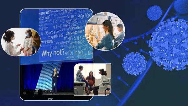 Read Ruth Porat's remarks on AI and cancer research at the American Society of Clinical Oncology.
 Learn how the 2025 Growth Academy: AI for Health cohort is building the next generation of healthcare solutions.
Learn how the 2025 Growth Academy: AI for Health cohort is building the next generation of healthcare solutions.
Learn how the 2025 Growth Academy: AI for Health cohort is building the next generation of healthcare solutions.
 Googler Thomas Wagner shares how he used Gemini to learn more about his son’s rare disease, and jumpstart research.
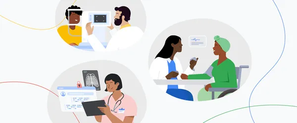 At The Check Up, we unveil how we’re using AI to reshape what’s possible in health and help people live healthier lives.
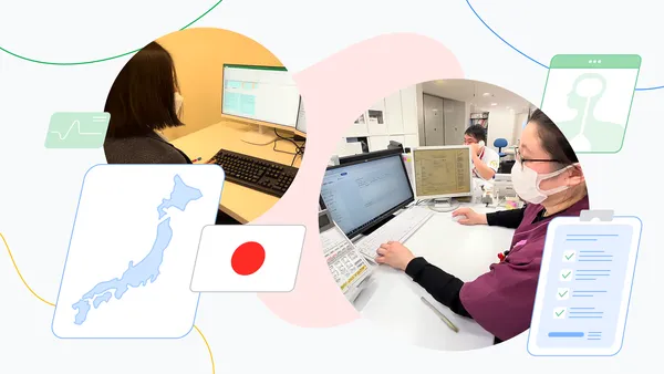 Ubie, a health tech startup in Japan, is using Google AI to change patient — and healthcare worker — experiences for the better.