Tag Archives: machine learning

Using Selective Attention in Reinforcement Learning Agents


Inattentional blindness is the psychological phenomenon that causes one to miss things in plain sight, and is a consequence of the selective attention that enables you to remain focused on important parts of the world without distraction from irrelevant details. It is believed that this selective attention mechanism enables people to condense broad sensory information into a form that is compact enough to be used for future decision making. While this may seem to be a limitation, such “bottlenecks” observed in nature can also inspire the design of machine learning systems that hope to mimic the success and efficiency of biological organisms. For example, while most methods presented in the deep reinforcement learning (RL) literature allow an agent to access the entire visual input, and even incorporating modules for predicting future sequences of visual inputs, perhaps reducing an agent’s access to its visual inputs via an attention constraint could be beneficial to an agent’s performance?

In our recent GECCO 2020 paper, “Neuroevolution of Self-Interpretable Agents” (AttentionAgent), we investigate the properties of such agents that employ a self-attention bottleneck. We show that not only are they able to solve challenging vision-based tasks from pixel inputs with 1000x fewer learnable parameters compared to conventional methods, they are also better at generalization to unseen modifications of their tasks, simply due to its ability to “not see details” that can confuse it. Furthermore, looking at where the agent is focusing its attention provides visual interpretability to its decision making process. The following diagram illustrates how the agent learned to deal with its attention bottleneck:
AttentionAgent learned to attend to task critical regions in its visual inputs. In a car driving task (CarRacing, top row), the agent mostly attends to the road borders, but shifts its focus to the turns before it changes heading directions. In a fireball dodging game (DoomTakeCover, bottom row), the agent focuses on fireballs and enemy monsters. Left: Visual inputs to the agent. Center: Agent’s attention overlaid on the visual inputs, the white patches indicate where the agent focuses its attention. Right: Visual cues based on which the agent makes decisions.
Agent with Artificial Attention
While there have been several works that explore how constraints such as sparsity may play a role in actually shaping the abilities of reinforcement learning agents, AttentionAgent takes inspiration from concepts related to inattentional blindness — when the brain is involved in effort-demanding tasks, it assigns most of its attention capacity only to task-relevant elements and is temporarily blind to other signals. To achieve this, we segment the input image into several patches and then rely on a modified self-attention architecture to simulate voting between patches to elect a subset to be considered important. The patches of interest are elected at each time step and, once determined, AttentionAgent makes decisions solely on these patches, ignoring the rest.

In addition to extracting key factors from visual inputs, the ability to contextualize these factors as they change in time is just as crucial. For example, a batter in the game of baseball must use visual signals to continuously keep track of the baseball's location in order to predict its position and be able to hit it. In AttentionAgent, a long short-term memory (LSTM) model accepts information from the important patches and generates an action at each time step. LSTM keeps track of the changes in the input sequence, and can thus utilize the information to track how critical factors evolve over time.

It is conventional to optimize a neural network with backpropagation. However, because AttentionAgent contains non-differentiable operations for the generation of important patches, like sorting and slicing, it is not straightforward to apply such techniques for training. We therefore turn to derivative-free optimization algorithms to overcome this difficulty.
Overview of our method and illustration of data processing flow in AttentionAgent. Top: Input transformation — A sliding window segments an input image into smaller patches, and then “flattens” them for future processing. Middle: Patch election — The modified self-attention module holds votes between patches to generate a patch importance vector. Bottom: Action generation — AttentionAgent picks the patches of the highest importance, extracts corresponding features and makes decisions based on them.
Generalization to Unseen Modifications of the Environment
We demonstrate that Attention Agent learned to attend to a variety of regions in the input images. Visualization of the important patches provides a peek into how the agent is making decisions, illustrating that most selections make sense and are consistent with human intuition, and is a powerful tool for analyzing and debugging an agent in development. Furthermore, since the agent learned to ignore information non-critical to the core task, it can generalize to tasks where small environmental modifications are applied.

Here, we show that restricting the agent’s decision-making controller’s access to important patches only while ignoring the rest of the scene can result in better generalization, simply due to how the agent is restricted from “seeing things” that can confuse it. Our agent is trained to survive in the VizDoom TakeCover environment only, but it can also survive in unseen settings with higher walls, different floor textures, or when confronted with a distracting sign.
DoomTakeCover Generalization: The AttentionAgent is trained in the environment with no modifications (left). It is able to adapt to changes in the environment, such as a higher wall (middle, left), a different floor texture (middle, right), or floating text (right).
When one learns to drive during a sunny day, one also can transfer those skills (to some extent) to driving at night, on a rainy day, in a different car, or in the presence of bird droppings on the windshield. AttentionAgent is not only able to solve CarRacing-v0, it can also achieve similar performance in unseen conditions, such as brighter or darker scenery, or having its vision modified by artifacts such as side bars or background blobs, while requiring 1000x fewer parameters than conventional methods that fail to generalize.
CarRacing Generalization: No modification (left); color perturbation (middle, left); vertical bars on left and right (middle, right); added red blob (right).
Limitations and Future Work
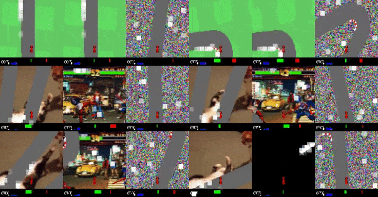
While AttentionAgent is able to cope with various modifications of the environment, there are limitations to this approach, and much more work to be done to further enhance the generalization capabilities of the agent. For example, AttentionAgent does not generalize to cases where dramatic background changes are involved. The agent trained on the original car racing environment with the green grass background fails to generalize when the background is replaced with distracting YouTube videos. When we take this one step further and replace the background with pure uniform noise, we observe that the agent’s attention module breaks down and attends only to random patches of noise, rather than to the road-related patches. If we train an agent from scratch in the noisy background environment, it manages to get around the track, although the performance is mediocre. Interestingly, the agent still attends only to the noise, rather than to the road, it appears to have learned to drive by estimating where the lane is based on the number of selected patches on the left and right of the screen.
AttentionAgent fails to generalize to drastically modified environments. Left: The background suddenly becomes a cat (Creative Commons video). Middle: The background suddenly becomes an arcade game (Creative Commons video). Right: AttentionAgent learned to drive on pure noise background by avoiding noise patches.
The simplistic method we use to extract information from important patches may be inadequate for more complicated tasks. How we can learn more meaningful features, and perhaps even extract symbolic information from the visual input will be an exciting future direction. In addition to open sourcing the code to the research community, we have also released CarRacingExtension, a suite of car racing tasks that involve various environmental modifications, as testbeds and benchmark for ML researchers who are interested in agent generalizations.

Acknowledgements
This research was conducted by Yujin Tang, Duong Nguyen, and David Ha. We would like to thank Yingtao Tian, Lana Sinapayen, Shixin Luo, Krzysztof Choromanski, Sherjil Ozair, Ben Poole, Kai Arulkumaran, Eric Jang, Brian Cheung, Kory Mathewson, Ankur Handa, and Jeff Dean for valuable discussions.

Source: Google AI Blog


Unlocking the "Chemome" with DNA-Encoded Chemistry and Machine Learning


Much of the development of therapeutics for human disease is built around understanding and modulating the function of proteins, which are the main workhorses of many biological activities. Small molecule drugs such as ibuprofen often work by inhibiting or promoting the function of proteins or their interactions with other biomolecules. Developing useful “virtual screening” methods where potential small molecules can be evaluated computationally rather than in a lab, has long been an area of research. However, the persistent challenge is to build a method that works well enough across a wide range of chemical space to be useful for finding small molecules with physically verified useful interaction with a protein of interest, i.e., “hits”.

In “Machine learning on DNA-encoded libraries: A new paradigm for hit-finding”, recently published in the Journal of Medicinal Chemistry, we worked in collaboration with X-Chem Pharmaceuticals to demonstrate an effective new method for finding biologically active molecules using a combination of physical screening with DNA-encoded small molecule libraries and virtual screening using a graph convolutional neural network (GCNN). This research has led to the creation of the Chemome initiative, a cooperative project between our Accelerated Science team and ZebiAI that will enable the discovery of many more small molecule chemical probes for biological research.

Background on Chemical Probes
Making sense of the biological networks that support life and produce disease is an immensely complex task. One approach to study these processes is using chemical probes, small molecules that aren’t necessarily useful as drugs, but that selectively inhibit or promote the function of specific proteins. When you have a biological system to study (such as cancer cells growing in a dish), you can add the chemical probe at a specific time and observe how the biological system responds differently when the targeted protein has increased or decreased activity. But, despite how useful chemical probes are for this kind of basic biomedical research, only 4% of human proteins have a known chemical probe available.

The process of finding chemical probes begins similarly to the earliest stages of small molecule drug discovery. Given a protein target of interest, the space of small molecules is scanned to find “hit” molecules that can be further tested. Robotic assisted high throughput screening where up to hundred of thousands or millions of molecules are physically tested is a cornerstone of modern drug research. However, the number of small molecules you can easily purchase (1.2x10⁹) is much larger than that, which in turn is much smaller than the number of small drug like molecules (estimates from 1020 to 1060). “Virtual screening” could possibly quickly and efficiently search this vast space of potentially synthesizable molecules and greatly speed up the discovery of therapeutic compounds.

DNA-Encoded Small Molecule Library Screening
The physical part of the screening process uses DNA-encoded small molecule libraries (DELs), which contain many distinct small molecules in one pool, each of which is attached to a fragment of DNA serving as a unique barcode for that molecule. While this basic technique has been around for several decades, the quality of the library and screening process is key to producing meaningful results.

DELs are a very clever idea to solve a biochemical challenge, which is how to collect small molecules into one place with an easy way to identify each. The key is to use DNA as a barcode to identify each molecule, similar to Nobel Prize winning phage display technology. First, one generates many chemical fragments, each with a unique DNA barcode attached, along with a common chemical handle (the NH2 in this case). The results are then pooled and split into separate reactions where a set of distinct chemical fragments with another common chemical handle (e.g., OH) are added. The chemical fragments from the two steps react and fuse together at the common chemical handles. The DNA fragments are also connected to build one continuous barcode for each molecule. The net result is that by performing 2N operations, one gets N2 unique molecules, each of which is identified by its own unique DNA barcode. By using more fragments or more cycles, it’s relatively easy to make libraries with millions or even billions of distinct molecules.
An overview of the process of creating a DNA encoded small molecule library. First, DNA “barcodes” (represented here with numbered helices) are attached to small chemical fragments (the blue shapes) which expose a common chemical “handle” (e.g. the NH2 shown here). When mixed with other chemical fragments (the orange shapes) each of which has another exposed chemical “handle” (the OH) with attached DNA fragments, reactions merge the sets of chemical and DNA fragments, resulting in a voluminous library of small molecules of interest, each with a unique DNA “barcode”.
Once the library has been generated, it can be used to find the small molecules that bind to the protein of interest by mixing the DEL together with the protein and washing away the small molecules that do not attach. Sequencing the remaining DNA barcodes produces millions of individual reads of DNA fragments, which can then be carefully processed to estimate which of the billions of molecules in the original DEL interact with the protein.

Machine Learning on DEL Data
Given the physical screening data returned for a particular protein, we build an ML model to predict whether an arbitrarily chosen small molecule will bind to that protein. The physical screening with the DEL provides positive and negative examples for an ML classifier. To simplify slightly, the small molecules that remain at the end of the screening process are positive examples and everything else are negative examples. We use a graph convolutional neural network, which is a type of neural network specially designed for small graph-like inputs, such as the small molecules in which we are interested.

Results
We physically screened three diverse proteins using DEL libraries: sEH (a hydrolase), ERα (a nuclear receptor), and c-KIT (a kinase). Using the DEL-trained models, we virtually screened large make-on-demand libraries from Mcule and an internal molecule library at X-Chem to identify a diverse set of molecules predicted to show affinity with each target. We compared the results of the GCNN models to a random forest (RF) model, a common method for virtual screening that uses standard chemical fingerprints, which we use as baseline. We find that the GCNN model significantly outperforms the RF model in discovering more potent candidates.
Fraction of molecules (“hit rates”) from those tested showing various levels of activity, comparing predictions from two different machine learned models (a GCNN and random forests, RF) on three distinct protein targets. The color scale on the right uses a common metric IC50 for representing the potency of a molecule. nM means “nanomolar” and µM means “micromolar”. Smaller values / darker colors are generally better molecules. Note that typical virtual screening approaches not built with DEL data normally only reach a few percent on this scale.
Importantly, unlike many other uses of virtual screening, the process to select the molecules to test was automated or easily automatable given the results of the model, and we did not rely on review and selection of the most promising molecules by a trained chemist. In addition, we tested almost 2000 molecules across the three targets, the largest published prospective study of virtual screening of which we are aware. While providing high confidence on the hit rates above, this also allows one to carefully examine the diversity of hits and the usefulness of the model for molecules near and far from the training set.

The Chemome Initiative
ZebiAI Therapeutics was founded based on the results of this research and has partnered with our team and X-Chem Pharmaceuticals to apply these techniques to efficiently deliver new chemical probes to the research community for human proteins of interest, an effort called the Chemome Initiative.

As part of the Chemome Initiative, ZebiAI will work with researchers to identify proteins of interest and source screening data, which our team will use to build machine learning models and make predictions on commercially available libraries of small molecules. ZebiAI will provide the predicted molecules to researchers for activity testing and will collaborate with researchers to advance some programs through discovery. Participation in the program requires that the validated hits be published within a reasonable time frame so that the whole community can benefit. While more validation must be done to make the hit molecules useful as chemical probes, especially for specifically targeting the protein of interest and the ability to function correctly in common assays, having potent hits is a big step forward in the process.

We’re excited to be a part of the Chemome Initiative enabled by the effective ML techniques described here and look forward to its discovery of many new chemical probes. We expect the Chemome will spur significant new biological discoveries and ultimately accelerate new therapeutic discovery for the world.

Acknowledgements
This work represents a multi-year effort between the Accelerated Science Team and X-Chem Pharmaceuticals with many people involved. This project would not have worked without the combined diverse skills of biologists, chemists, and ML researchers. We should especially acknowledge Eric Sigel (of X-Chem, now at ZebiAI) and Kevin McCloskey (of Google), the first authors on the paper and Steve Kearnes (of Google) for core modelling ideas and technical work.

Source: Google AI Blog


Recent Advances in Google Translate


Advances in machine learning (ML) have driven improvements to automated translation, including the GNMT neural translation model introduced in Translate in 2016, that have enabled great improvements to the quality of translation for over 100 languages. Nevertheless, state-of-the-art systems lag significantly behind human performance in all but the most specific translation tasks. And while the research community has developed techniques that are successful for high-resource languages like Spanish and German, for which there exist copious amounts of training data, performance on low-resource languages, like Yoruba or Malayalam, still leaves much to be desired. Many techniques have demonstrated significant gains for low-resource languages in controlled research settings (e.g., the WMT Evaluation Campaign), however these results on smaller, publicly available datasets may not easily transition to large, web-crawled datasets.

In this post, we share some recent progress we have made in translation quality for supported languages, especially for those that are low-resource, by synthesizing and expanding a variety of recent advances, and demonstrate how they can be applied at scale to noisy, web-mined data. These techniques span improvements to model architecture and training, improved treatment of noise in datasets, increased multilingual transfer learning through M4 modeling, and use of monolingual data. The quality improvements, which averaged +5 BLEU score over all 100+ languages, are visualized below.
BLEU score of Google Translate models since shortly after its inception in 2006. The improvements since the implementation of the new techniques over the last year are highlighted at the end of the animation.
Advances for Both High- and Low-Resource Languages
Hybrid Model Architecture: Four years ago we introduced the RNN-based GNMT model, which yielded large quality improvements and enabled Translate to cover many more languages. Following our work decoupling different aspects of model performance, we have replaced the original GNMT system, instead training models with a transformer encoder and an RNN decoder, implemented in Lingvo (a TensorFlow framework). Transformer models have been demonstrated to be generally more effective at machine translation than RNN models, but our work suggested that most of these quality gains were from the transformer encoder, and that the transformer decoder was not significantly better than the RNN decoder. Since the RNN decoder is much faster at inference time, we applied a variety of optimizations before coupling it with the transformer encoder. The resulting hybrid models are higher-quality, more stable in training, and exhibit lower latency.

Web Crawl: Neural Machine Translation (NMT) models are trained using examples of translated sentences and documents, which are typically collected from the public web. Compared to phrase-based machine translation, NMT has been found to be more sensitive to data quality. As such, we replaced the previous data collection system with a new data miner that focuses more on precision than recall, which allows the collection of higher quality training data from the public web. Additionally, we switched the web crawler from a dictionary-based model to an embedding based model for 14 large language pairs, which increased the number of sentences collected by an average of 29 percent, without loss of precision.

Modeling Data Noise: Data with significant noise is not only redundant but also lowers the quality of models trained on it. In order to address data noise, we used our results on denoising NMT training to assign a score to every training example using preliminary models trained on noisy data and fine-tuned on clean data. We then treat training as a curriculum learning problem — the models start out training on all data, and then gradually train on smaller and cleaner subsets.

Advances That Benefited Low-Resource Languages in Particular
Back-Translation: Widely adopted in state-of-the-art machine translation systems, back-translation is especially helpful for low-resource languages, where parallel data is scarce. This technique augments parallel training data (where each sentence in one language is paired with its translation) with synthetic parallel data, where the sentences in one language are written by a human, but their translations have been generated by a neural translation model. By incorporating back-translation into Google Translate, we can make use of the more abundant monolingual text data for low-resource languages on the web for training our models. This is especially helpful in increasing fluency of model output, which is an area in which low-resource translation models underperform.

M4 Modeling: A technique that has been especially helpful for low-resource languages has been M4, which uses a single, giant model to translate between all languages and English. This allows for transfer learning at a massive scale. As an example, a lower-resource language like Yiddish has the benefit of co-training with a wide array of other related Germanic languages (e.g., German, Dutch, Danish, etc.), as well as almost a hundred other languages that may not share a known linguistic connection, but may provide useful signal to the model.

Judging Translation Quality
A popular metric for automatic quality evaluation of machine translation systems is the BLEU score, which is based on the similarity between a system’s translation and reference translations that were generated by people. With these latest updates, we see an average BLEU gain of +5 points over the previous GNMT models, with the 50 lowest-resource languages seeing an average gain of +7 BLEU. This improvement is comparable to the gain observed four years ago when transitioning from phrase-based translation to NMT.

Although BLEU score is a well-known approximate measure, it is known to have various pitfalls for systems that are already high-quality. For instance, several works have demonstrated how the BLEU score can be biased by translationese effects on the source side or target side, a phenomenon where translated text can sound awkward, containing attributes (like word order) from the source language. For this reason, we performed human side-by-side evaluations on all new models, which confirmed the gains in BLEU.

In addition to general quality improvements, the new models show increased robustness to machine translation hallucination, a phenomenon in which models produce strange “translations” when given nonsense input. This is a common problem for models that have been trained on small amounts of data, and affects many low-resource languages. For example, when given the string of Telugu characters “ష ష ష ష ష ష ష ష ష ష ష ష ష ష ష”, the old model produced the nonsensical output “Shenzhen Shenzhen Shaw International Airport (SSH)”, seemingly trying to make sense of the sounds, whereas the new model correctly learns to transliterate this as “Sh sh sh sh sh sh sh sh sh sh sh sh sh sh sh sh sh”.

Conclusion
Although these are impressive strides forward for a machine, one must remember that, especially for low-resource languages, automatic translation quality is far from perfect. These models still fall prey to typical machine translation errors, including poor performance on particular genres of subject matter (“domains”), conflating different dialects of a language, producing overly literal translations, and poor performance on informal and spoken language.

Nonetheless, with this update, we are proud to provide automatic translations that are relatively coherent, even for the lowest-resource of the 108 supported languages. We are grateful for the research that has enabled this from the active community of machine translation researchers in academia and industry.

Acknowledgements
This effort is built on contributions from Tao Yu, Ali Dabirmoghaddam, Klaus Macherey, Pidong Wang, Ye Tian, Jeff Klingner, Jumpei Takeuchi, Yuichiro Sawai, Hideto Kazawa, Apu Shah, Manisha Jain, Keith Stevens, Fangxiaoyu Feng, Chao Tian, John Richardson, Rajat Tibrewal, Orhan Firat, Mia Chen, Ankur Bapna, Naveen Arivazhagan, Dmitry Lepikhin, Wei Wang, Wolfgang Macherey, Katrin Tomanek, Qin Gao, Mengmeng Niu, and Macduff Hughes.

Source: Google AI Blog


Building a more resilient world together

Posted by Billy Rutledge, Director of the Coral team

UNDP Hackster.io COVID19 Detect Protect Poster

Recently, we’ve seen communities respond to the challenges of the coronavirus pandemic by using technology in new ways to effect positive change. It’s increasingly important that our systems are able to adapt to new contexts, handle disruptions, and remain efficient.

At Coral, we believe intelligence at the edge is a key ingredient towards building a more resilient future. By making the latest machine learning tools easy-to-use and accessible, innovators can collaborate to create solutions that are most needed in their communities. Developers are already using Coral to build solutions that can understand and react in real-time, while maintaining privacy for everyone present.

Helping our communities stay safe, together

As mandatory isolation measures begin to relax, compliance with safe social distancing protocol has become a topic of primary concern for experts across the globe. Businesses and individuals have been stepping up to find ways to use technology to help reduce the risk and spread. Many efforts are employing the benefits of edge AI—here are a few early stage examples that have inspired us.

woman and child crossing the street

In Belgium, engineers at Edgise recently used Coral to develop an occupancy monitor to aid businesses in managing capacity. With the privacy preserving properties of edge AI, businesses can anonymously count how many customers enter and exit a space, signaling when the area is too full.

A research group at the Sathyabama Institute of Science and Technology in India are using Coral to develop a wearable device to serve as a COVID-19 cough counter and health monitor, allowing medical professionals to better care for low risk patients in an outpatient capacity. Coral's Edge TPU enables biometric data to be processed efficiently, without draining the limited power resources available in wearable devices.

All across the US, hospitals are seeking solutions to ensure adherence to hygiene policy amongst hospital staff. In one example, a device incorporates the compact, affordable and offline benefits of the Coral modules to aid in handwashing practices at numerous stations throughout a facility.

And around the world, members of the PyImageSearch community are exploring how to train a COVID-19: Face Mask Detector model using TensorFlow that can be used to identify whether people are wearing a mask. Open source frameworks can empower anyone to develop solutions, and with Coral components we can help bring those benefits to everyone.

Eliciting a global response

In an effort to rally greater community involvement, Coral has joined The United Nations Development Programme and Hackster.io, as a sponsor of the COVID-19 Detect and Protect Challenge. The initiative calls on developers to build affordable and reproducible solutions that support response efforts in developing countries. All ideas are welcome—whether they use ML or not—and we encourage you to participate.

To make edge ML capabilities even easier to integrate, we’re also announcing a price reduction for the Coral products widely used for experimentation and prototyping. Our Dev Board will now be offered at $129.99, the USB Accelerator at $59.99, the Camera Module at $19.99, and the Enviro Board at $14.99. Additionally, we are introducing the USB Accelerator into 10 new markets: Ghana, Thailand, Singapore, Oman, Philippines, Indonesia, Kenya, Malaysia, Israel, and Vietnam. For more details, visit Coral.ai/products.

We’re excited to see the solutions developers will bring forward with Coral. And as always, please keep sending us feedback at [email protected].

Speeding Up Neural Network Training with Data Echoing


Over the past decade, dramatic increases in neural network training speed have made it possible to apply deep learning techniques to many important problems. In the twilight of Moore's law, as improvements in general purpose processors plateau, the machine learning community has increasingly turned to specialized hardware to produce additional speedups. For example, GPUs and TPUs optimize for highly parallelizable matrix operations, which are core components of neural network training algorithms. These accelerators, at a high level, can speed up training in two ways. First, they can process more training examples in parallel, and second, they can process each training example faster. We know there are limits to the speedups from processing more training examples in parallel, but will building ever faster accelerators continue to speed up training?

Unfortunately, not all operations in the training pipeline run on accelerators, so one cannot simply rely on faster accelerators to continue driving training speedups. For example, earlier stages in the training pipeline like disk I/O and data preprocessing involve operations that do not benefit from GPUs and TPUs. As accelerator improvements outpace improvements in CPUs and disks, these earlier stages will increasingly become a bottleneck, wasting accelerator capacity and limiting training speed.
An example training pipeline representative of many large-scale computer vision programs. The stages that come before applying the mini-batch stochastic gradient descent (SGD) update generally do not benefit from specialized hardware accelerators.
Consider a scenario where the code upstream to the accelerator takes twice as long as the code that runs on the accelerator – a scenario that is already realistic for some workloads today. Even if the code is pipelined to execute the upstream and downstream stages in parallel, the upstream stage will dominate training time and the accelerator will be idle 50% of the time. In this case, building a faster accelerator will not improve training speed at all. It may be possible to speed up the input pipeline by dedicating engineering effort and additional compute resources, but such efforts are time consuming and distract from the main goal of improving predictive performance. For very small datasets,one can precompute the augmented dataset offline and load the entire preprocessed dataset in memory, but this doesn’t work for most ML training scenarios.

In “Faster Neural Network Training with Data Echoing”, we propose a simple technique that reuses (or “echoes”) intermediate outputs from earlier pipeline stages to reclaim idle accelerator capacity. Rather than waiting for more data to become available, we simply utilize data that is already available to keep the accelerators busy.
Left: Without data echoing, downstream computational capacity is idle 50% of the time. Right: Data echoing with echoing factor 2 reclaims downstream computational capacity.
Repeating Data to Train Faster
Imagine a situation where reading and preprocessing a batch of training data takes twice as long as performing a single optimization step on that batch. In this case, after the first optimization step on the preprocessed batch, we can reuse the batch and perform a second step before the next batch is ready. In the best case scenario, where repeated data is as useful as fresh data, we would see a twofold speedup in training. In reality, data echoing provides a slightly smaller speedup because repeated data is not as useful as fresh data – but it can still provide a significant speedup compared to leaving the accelerator idle.

There are typically several ways to implement data echoing in a given neural network training pipeline. The technique we propose involves duplicating data into a shuffle buffer somewhere in the training pipeline, but we are free to insert this buffer anywhere after whichever stage produces a bottleneck in the given pipeline. When we insert the buffer before batching, we call our technique example echoing, whereas, when we insert it after batching, we call our technique batch echoing. Example echoing shuffles data at the example level, while batch echoing shuffles the sequence of duplicate batches. We can also insert the buffer before data augmentation, such that each copy of repeated data is slightly different (and therefore closer to a fresh example). Of the different versions of data echoing that place the shuffle buffer between different stages, the version that provides the greatest speedup depends on the specific training pipeline.

Data Echoing Across Workloads
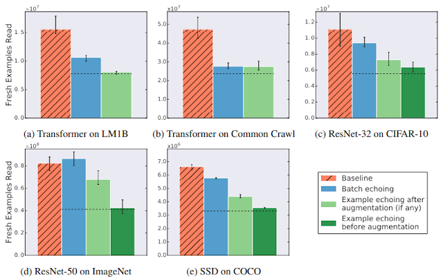
So how useful is reusing data? We tried data echoing on five neural network training pipelines spanning 3 different tasks – image classification, language modeling, and object detection – and measured the number of fresh examples needed to reach a particular performance target. We chose targets to match the best result reliably achieved by the baseline during hyperparameter tuning. We found that data echoing allowed us to reach the target performance with fewer fresh examples, demonstrating that reusing data is useful for reducing disk I/O across a variety of tasks. In some cases, repeated data is nearly as useful as fresh data: in the figure below, example echoing before augmentation reduces the number of fresh examples required almost by the repetition factor.
Data echoing, when each data item is repeated twice, either reduces or does not change the number of fresh examples needed to reach the target out-of-sample performance. Dashed lines indicate the values we would expect if repeated examples were as useful as fresh examples.
Reduction in Training Time
Data echoing can speed up training whenever computation upstream from accelerators dominates training time. We measured the training speedup achieved in a training pipeline bottlenecked by input latency due to streaming training data from cloud storage, which is realistic for many of today’s large-scale production workloads or anyone streaming training data over a network from a remote storage system. We trained a ResNet-50 model on the ImageNet dataset and found that data echoing provides a significant training speedup, in this case, more than 3 times faster when using data echoing.
Data echoing can reduce training time for ResNet-50 on ImageNet. In this experiment, reading a batch of training data from cloud storage took 6 times longer than the code that used each batch of data to perform a training step. The Echoing factor in the legend refers to the number of times each data item was repeated. Dashed lines indicate the expected values if repeated examples were as useful as fresh examples and there was no overhead from echoing.
Data Echoing Preserves Predictive Performance
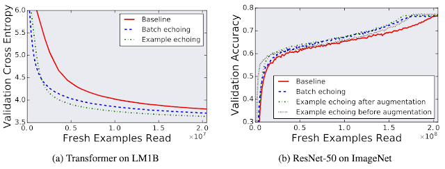
Although one might be concerned that reusing data would harm the model’s final performance, we found that data echoing did not degrade the quality of the final model for any of the workloads we tested.
Comparing the individual trials that achieved the best out-of-sample performance during training for both with and without data echoing shows that reusing data does not harm final model quality. Here validation cross entropy is equivalent to log perplexity.
As improvements in specialized accelerators like GPUs and TPUs continue to outpace general purpose processors, we expect data echoing and similar strategies to become increasingly important parts of the neural network training toolkit.

Acknowledgements
The Data Echoing project was conducted by Dami Choi, Alexandre Passos, Christopher J. Shallue, and George E. Dahl while Dami Choi was a Google AI Resident. We would also like to thank Roy Frostig, Luke Metz, Yiding Jiang, and Ting Chen for helpful discussions.

Source: Google AI Blog


Agile and Intelligent Locomotion via Deep Reinforcement Learning


Recent advancements in deep reinforcement learning (deep RL) has enabled legged robots to learn many agile skills through automated environment interactions. However, the lack of sample efficiency is still a major bottleneck for many algorithms, and researchers have to rely on using off-policy data, imitating animal behaviors, or performing meta learning to reduce the amount of real world experience required. Moreover, most existing works focus on simple, low-level skills only, such as walking forward, backward and turning. In order to operate autonomously in the real world, robots still need to combine these skills to generate more advanced behaviors.

Today we present two projects that aim to address the above problems and help close the perception-actuation loop for legged robots. In “Data Efficient Reinforcement Learning for Legged Robots”, we present an efficient way to learn low level motion control policies. By fitting a dynamics model to the robot and planning for actions in real time, the robot learns multiple locomotion skills using less than 5 minutes of data. Going beyond simple behaviors, we explore automatic path navigation in “Hierarchical Reinforcement Learning for Quadruped Locomotion”. With a policy architecture designed for end-to-end training, the robot learns to combine a high-level planning policy with a low-level motion controller, in order to navigate autonomously through a curved path.

Data Efficient Reinforcement Learning for Legged Robots
A major roadblock in RL is the lack of sample efficiency. Even with a state-of-the-art sample-efficient learning algorithm like Soft Actor-Critic (SAC), it would still require more than an hour of data to learn a reasonable walking policy, which is difficult to collect in the real world.

In a continued effort to learn walking skills using minimal interaction with the real-world environment, we present a model-based method to learn basic walking skills. Instead of directly learning a policy that maps from environment state to robot action, we learn a dynamics model of the robot that estimates future states given its current state and action. Since the entire learning process requires less than 5 minutes of data, it could be performed directly on the real robot.

We start by executing random actions on the robot, and fit the model to the data collected. With the model fitted, we control the robot using a model predictive control (MPC) planner. We iterate between collecting more data with MPC and re-training the model to better fit the dynamics of the environment.
Overview of the model-based learning pipeline. The system alternates between fitting the dynamics model and collecting trajectories using model predictive control (MPC).
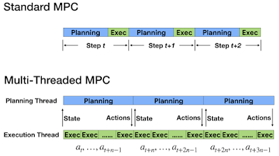
In standard MPC, the controller plans for a sequence of actions at each timestep, and only executes the first of the planned actions. While online replanning with regular feedback from the robot to the controller makes the controller robust to model inaccuracies, it also poses a challenge for the action planner, as planning must finish before the next step of the control loop (usually less than 10ms for legged robots). To satisfy such a tight time constraint, we introduce a multi-threaded, asynchronous version of MPC, with action planning and execution happening on different threads. As the execution thread applies actions at a high frequency, the planning thread optimizes for actions in the background without interruption. Furthermore, since action planning can take multiple timesteps, the robot state would have changed by the time planning has finished. To address the problem with planning latency, we devise a novel technique to compensate, which first predicts the future state when the planner is expected to finish its computation, and then uses this future state to seed the planning algorithm.
We separate action planning and execution on different threads.
Although MPC refreshes the action plan frequently, the planner still needs to work over long action horizons to keep track of the long-term goal and avoid myopic behaviors. To that end, we use a multi-step loss function, a reformulation of the model loss function that helps to reduce error accumulation over time by predicting the loss over a range of future steps.

Safety is another concern for learning on the real robot. For legged robots, a small mistake, such as missing a foot step, could lead to catastrophic failures, from the robot falling to the motor overheating. To ensure safe exploration, we embed a stable, in-place stepping gait prior, that is modulated by a trajectory generator. With the stable walking prior, MPC can then safely explore the action space.

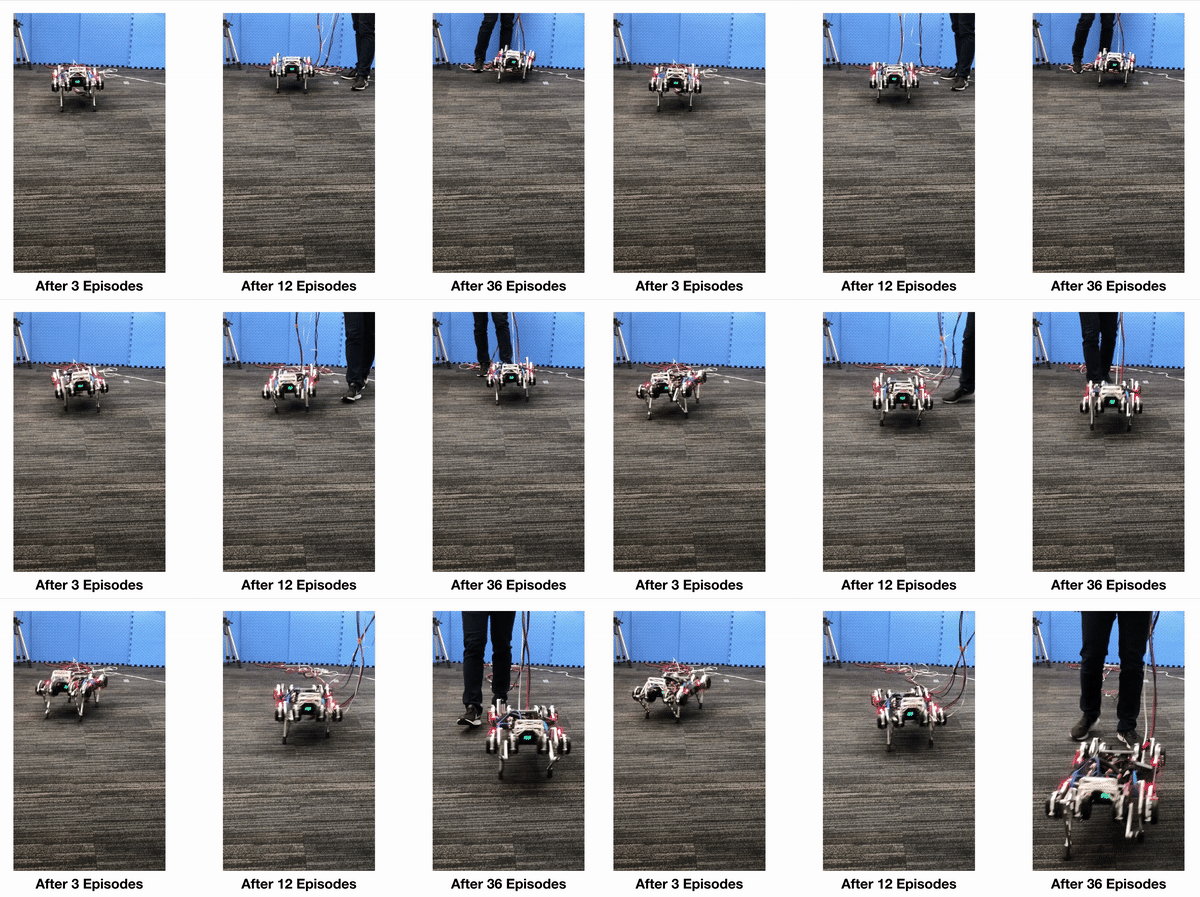
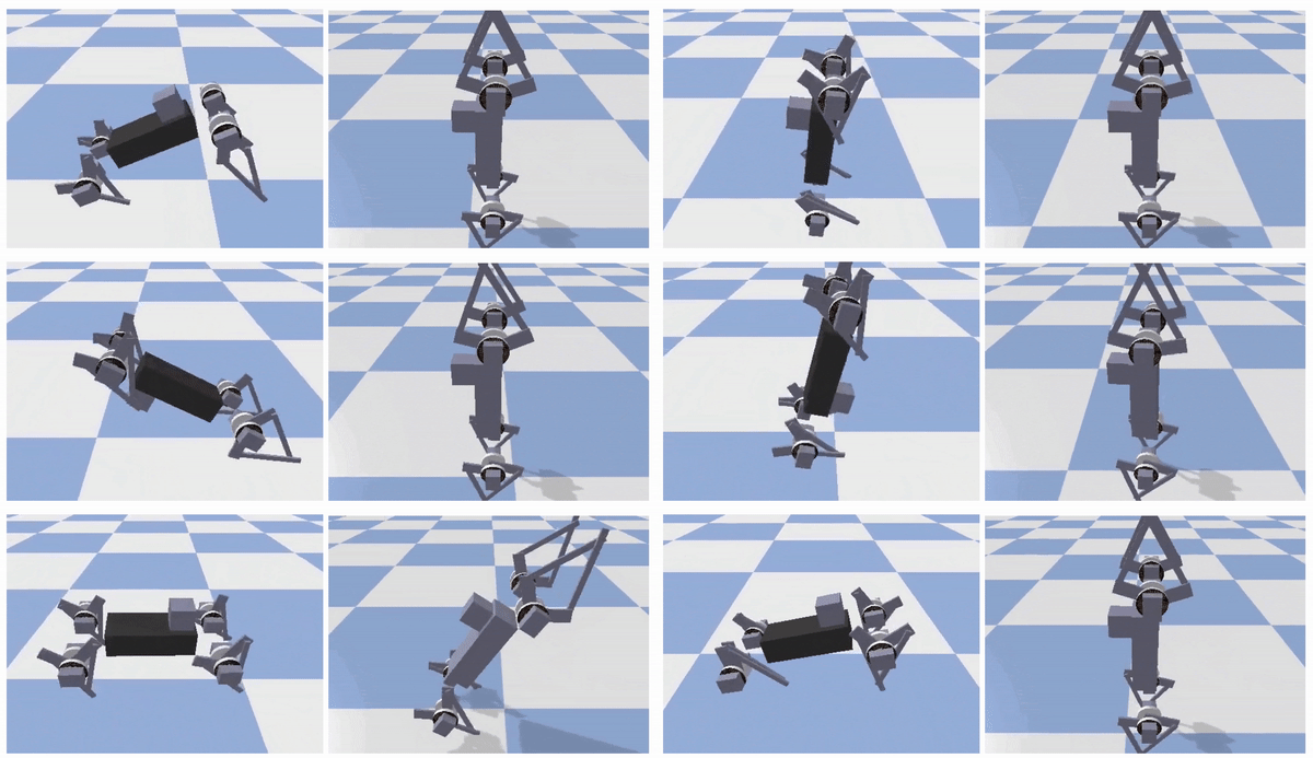
Combining an accurate dynamics model with an online, asynchronous MPC controller, the robot successfully learned to walk using only 4.5 minutes of data (36 episodes). The learned dynamics model is also generalizable: by simply changing the reward function of MPC, the controller is able to optimize for different behaviors, such as walking backwards, or turning, without re-training. As an extension, we use a similar framework to enable even more agile behaviors. For example, in simulation the robot learns to backflip and walk on its rear legs, though these behaviors are yet to be learned by the real robot.
The robot learns to walk using only 4.5 minutes of data.
The robot learns to backflip and walk with rear legs using the same framework.
Combining low-level controller with high-level planning
Although model-based RL has allowed the robot to learn simple locomotion skills efficiently, such skills are insufficient for handling complex, real-world tasks. For example, in order to navigate through an office space, the robot may have to adjust its speed, direction and height multiple times, instead of following a pre-defined speed profile. Traditionally, people solve such complex tasks by breaking them down into multiple hierarchical sub-problems, such as a high-level trajectory planner and a low-level trajectory-following controller. However, manually defining a suitable hierarchy is typically a tedious task, as it requires careful engineering for each sub-problem.

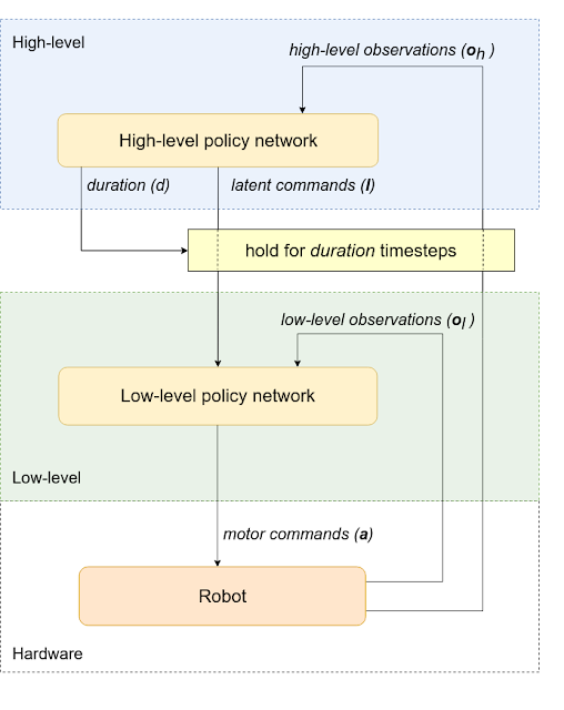
In our second paper, we introduce a hierarchical reinforcement learning (HRL) framework that can be trained to automatically decompose complex reinforcement learning tasks. We break down our policy structure into a high-level and a low-level policy. Instead of designing each policy manually, we only define a simple communication protocol between the policy levels. In this framework, the high-level policy (e.g., a trajectory planner) commands the low-level policy (such as the motion control policy) through a latent command, and decides for how long to hold that command constant before issuing a new one. The low-level policy then interprets the latent command from the high-level policy, and gives motor commands to the robot.

To facilitate learning, we also split the observation space into high-level (e.g., robot position and orientation) and low-level (IMU, motor positions) observations, which are fed to their corresponding policies. This architecture naturally allows the high-level policy to operate at a slower timescale than the low-level policy, which saves computation resources and reduces training complexity.
Framework of Hierarchical Policy: The policy gets observations from the robot and sends motor commands to execute desired actions. It is split into two levels (high and low). The high-level policy gives a latent command to the low-level policy and also decides the duration for which low-level will run.
Since the high-level and low-level policies operate at discrete timescales, the entire policy structure is not end-to-end differentiable, and standard gradient-based RL algorithms like PPO and SAC cannot be used. Instead, we choose to train the hierarchical policy through augmented random search (ARS), a simple evolutionary optimization method that has demonstrated good performance in reinforcement learning tasks. Weights of both levels of the policy are trained together, where the objective is to maximize the total reward from the robot trajectory.

We test our framework on a path-following task using the same quadruped robot. In addition to straight walking, the robot needs to steer in different directions to complete the task. Note that as the low-level policy does not know the robot’s position in the path, it does not have sufficient information to complete the entire task on its own. However, with the coordination between the high-level and low-level policies, steering behavior emerges automatically in the latent command space, which allows the robot to efficiently complete the path. After successful training in a simulated environment, we validate our results on hardware by transferring an HRL policy to a real robot and recording the resulting trajectories.
Successful trajectory of a robot on a curved path. Left: A plot of the trajectory traversed by the robot with dots along the trajectory marking the positions where the high-level policy sent a new latent command to the low-level policy. Middle: The robot walking along the path in the simulated environment. Right: The robot walking around the path in the real world.
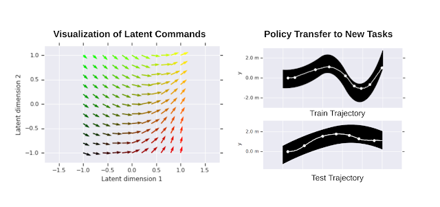
To further demonstrate the learned hierarchical policy, we visualized the behavior of the learned low-level policy under different latent commands. As shown in the plot below, different latent commands can cause the robot to walk straight, or turn left or right at different rates. We also test the generalizability of low-level policies by transferring them to new tasks from a similar domain, which, in our case, includes following a path with different shapes. By fixing the low-level policy weights and only training the high-level policy, the robot could successfully traverse through different paths.
Left: Visualization of a learned 2D latent command space. Vector directions correspond to the movement direction of the robot. Vector length is proportional to the distance covered. Right: Transfer of low level policy: An HRL policy was trained on a single path (right, top). The learned low-level policy was then reused when training the high-level policy on other paths (e.g., right, bottom).
Conclusion
Reinforcement learning poses a promising future for robotics by automating the controller design process. With model-based RL, we enabled efficient learning of generalizable locomotion behaviors directly on the real robot. With hierarchical RL, the robot learned to coordinate policies at different levels to achieve more complex tasks. In the future, we plan to bring perception into the loop, so that robots can operate truly autonomously in the real world.

Acknowledgements
Both Deepali Jain and Yuxiang Yang are residents in the AI Residency program, mentored by Ken Caluwaerts and Atil Iscen. We would also like to thank Jie Tan and Vikas Sindhwani for support of the research, and Noah Broestl for managing the New York AI Residency Program.

Source: Google AI Blog


Understanding the Shape of Large-Scale Data


Understanding the differences and similarities between complex datasets is an interesting challenge that often arises when working with data. One way to formalize this question is to view each dataset as a graph, a mathematical model for how items relate to each other. Graphs are widely used to model relationships between objects — the Internet graph connects pages referencing each other, social graphs link together friends, and molecule graphs connect atoms bonding with each other.
Graphs are discrete objects that can model the relationships between many different types of data, including web pages (left), social connections (center), or molecules (right).
Once there is a collection of multiple graphs, it is common to want to predict some property of each one as an aggregate (i.e., one label per graph). For example, consider the task of predicting protein function from structure: each dataset here is one protein, and the prediction task is whether the final structure encodes an enzyme or not. Since one wants a model to actually compute the prediction, we need a representation that lets us generalize across different protein structures. Ideally, one would want a way to represent graphs as vectors without costly labelling. The problem becomes harder with increasing graph size — in the molecule case humans possess some knowledge about their properties, however, reasoning about larger, more complex datasets becomes increasingly difficult.

In this post we highlight some recent advances in the area of graph representation learning with “Just SLaQ When You Approximate: Accurate Spectral Distances for Web-Scale Graphs” (published at WWW'20), a publication that improves on the scalability of our earlier research, “DDGK: Learning Graph Representations for Deep Divergence Graph Kernels” (published at WWW’19). SLaQ introduces a way to scale computations to approximate a certain class of graph statistics, allowing one to quickly and efficiently characterize large graphs. We are also happy to announce that we have released the code for both papers in the Google Research GitHub repository for graph embeddings.

Fully Unsupervised Learning of Graph Similarity
In our 2019 paper, we showed that it is possible to learn representations for graph similarity with neither domain knowledge nor supervision. We propose deep divergence graph kernels (DDGK), an unsupervised method for learning representations over graphs that encode mappings of similarities between them. Unlike previous work, our unsupervised method jointly learns node representations, graph representations, and an attention-based alignment between graphs.
Here is a t-SNE visualization of the latent representations learned by DDGK to compare proteins. Blue points indicate proteins that encode enzymes and the red points are for those that do not. We can see that the encoding correlates with a structural property of the protein (whether or not it encodes enzymes), even though this context was not provided during training. (Note that this is a projection of the representations, and so the absolute axis values aren’t meaningful.)
In the example above, we demonstrate how these representations can automatically learn to represent graphs and align them in a way that encodes their latent functional similarity. Experiments on other datasets show we can capture similarities and differences across graphs of different types (language, biology, and social interactions).
The pairwise distance between different datasets encoded and aligned using DDGK. Color indicates distance in the latent space, and the scale of similarity ranges from 0 (identical) to 1.0 (very different). We see that the representations can be clustered to group similar datasets together — for example, the datasets nci1 and ptc are both datasets of chemical compounds.
Fast and Accurate Approximation of Spectral Descriptors
A graph’s spectrum is a powerful representation that encodes its properties, including connectivity patterns between graph nodes and clustering information. The spectrum has been shown to convey rich information about the properties of different objects such as the sound of a drum, 3D shapes, graphs, and general high-dimensional data. Applications of spectral graph descriptors include AutoML systems, anomaly detection in dynamic graphs, and chemical molecule characterization.

Currently, learning-based systems such as DDGK do not scale to either large graphs or large graph collections. Alternatively, one can use the spectral information without the learning component to attain more desirable scaling properties. However, computing spectral descriptors for large graphs is computationally prohibitive. Our more recent paper addresses this problem by proposing SLaQ, a method for approximating a family of graph descriptors. Our approach uses a randomized approximation algorithm for computing traces of spectrum functions that allows us to study several well-known spectral graph characteristics like Von Neumann Graph Entropy, Estrada Index, graph energy, and NetLSD.

For example, we use SLaQ to monitor anomalous changes in the Wikipedia graph structure. SLaQ allows us to discern meaningful changes in the structure of the page graph from trivial ones such as mass page renames. Our experiments show two orders of magnitude improvement in approximation accuracy, on average.
Left: The well-known Karate graph represents the social interactions of two martial arts clubs. Right: The spectral descriptors (NetLSD, VNGE, and Estrada Index) computed for the original graph in blue and the version with removed edges in red.
Conclusions
Unsupervised representation learning for graphs is an important problem, and we believe that the methods we highlight here are exciting steps forward in this area! Specifically, SLaQ allows us to compute principled representations for vast datasets, and DDGK introduces a mechanism for automatically learning alignments between datasets. We hope that our contributions will help advance the analysis of large datasets, and will be useful for understanding changes to time-varying graph datasets, like those used in recommendation systems.

Acknowledgements
We thank Marina Munkhoeva, Rami Al-Rfou, and Dustin Zelle who contributed to these works. For more information on the Graph Mining team (part of Algorithm and Optimization Group) visit our pages.

Source: Google AI Blog


Applying Machine Learning to…..Yeast?


Humans have a long history with yeast, tied to the beginnings of plant domestication — baker’s (or brewer’s) yeast, Saccharomyces cerevisiae, has been used to make grains more digestible in the form of bread (or beer) for millennia. Today, yeast still has a large impact, with biologists adopting it as a model organism for biological research, genetics in particular, because it is easy to grow in the lab and is a eukaryote (i.e., unlike bacteria, it has a cell nucleus, like our cells do). It has even earned its own catchphrase in the biological community — “the awesome power of yeast genetics”. Studying the fundamentals of genetics is much easier in yeast, but is still applicable to humans since ~1000 yeast genes have a sequence homolog to human ones. Understanding how genes work together as a system is core to understanding all living things, which drives interest in this microorganism.

In collaboration with Calico Life Sciences, we present “Learning causal networks using inducible transcription factors and transcriptome-wide time series”, published in Molecular Systems Biology. Based on exhaustive experiments, we built a genome-wide model for the regulation of gene expression in S. cerevisiae and verified some of the results experimentally, enabling future investigations into less well understood biological systems. The Induction Dynamics gene Expression Atlas is available from Calico in a format easy to manipulate in python, with open-sourced code to do this on the Google Research GitHub. The data is hosted in a standard format at the Gene Expression Omnibus.

Using Yeast to Provide Insight into Aging
Yeast reproduce through a process called budding, in which a small bud grows from the surface of the parent to produce an offspring that is almost genetically identical. Interestingly, even though yeast are single-celled organisms, they grow old and die, typically after 30 budding events. In fact the “scars” from budding are clearly visible under a powerful microscope, allowing one to tell the age of the cell simply by looking! The problem is that researchers still do not know what causes aging to happen.
Bud scars on old yeast cells (5 μm bar for scale) — Photo Credit: Ian Foe, (Calico)
Scientists at Calico Life Sciences have pioneered a technique to make targeted perturbations to gene expression in yeast (i.e., allowing them to selectively “turn on” a gene’s activity) with the goal of understanding how aging works at the molecular level. The hope is that understanding aging in yeast will apply to aging in more complex organisms, like humans. This work is an early step in building a predictive framework for understanding the behavior of cells over time.

The Gene Expression Experiment
Genes encoded in DNA only function after being transcribed to RNA. It’s the RNA that is “translated” or “read” by ribosomes to produce protein. The level of protein production is governed by how much RNA is transcribed from DNA. Most of the work in a cell is being done by proteins, so they are key to understanding cell behavior. Yet, while we’d really like to measure the protein production levels, techniques to identify proteins at this scale are prohibitively expensive. Instead, in this experiment we use RNA as a proxy, since measuring RNA levels is easier.

The gene expression experiment is designed to perturb individual genes and measure, over time, how every other gene in the genome responds. The ability to rapidly perturb and track dynamics allows us to learn causal relationships and non-linear behaviors missing in most experiments. These dynamic data can also be used to train predictive models. This is made possible by strains of yeast with a single gene that is responsive to an external switch, in this case the hormone β-estradiol. To perturb a gene, the hormone is introduced, causing the switched gene to be overexpressed by a factor of 50 within 10 minutes. The yeast culture is then sampled at several points in time to measure the gene expression levels on microarrays. These experiments were done in parallel, with one yeast strain per culture, running concurrently.

Most of the perturbation experiments were done on a particular class of genes coding for transcription factors (TFs). These genes are the primary regulators of gene expression, coding for proteins that actually bind to the DNA strands, permitting or blocking transcription of particular genes.

When gene “a” is turned on it may upregulate gene “b” and downregulate gene “c”, and later lead to upregulation of gene “d”. Since yeast has more than 6000 genes, tracing the downstream impact of perturbing a single gene can get complicated very quickly. By combining experiments on different genes, one hopes to disambiguate the exact regulation mechanisms.
Schematic of the genome perturbation experiment: yeast strain with switchable gene “a”. Turning on a single gene (A) can result in differing levels of gene expression over time (B). Tracking these changes in comparison to those induced by turning on other genes (C and D) can provide insight into the regulation mechanisms (E).
The Gene Expression Model
For this experiment, we partnered with Calico because of the scale of the data, and the opportunity to leverage Google’s machine learning expertise and compute resources. There were more than 200 perturbation experiments on different yeast strains, each activating a single gene. In each experiment, the expression levels of all 6000 genes were measured eight times over 90 minutes, yielding a total of almost 20 million individual measurements (panel F, above). Clearly some automation was required to analyze the data.

Our approach was to model the whole process as a system of differential equations: the rate of change of the expression of a gene was proportional to a weighted sum of the expression levels of all genes. We first estimated the time derivatives from the data by simply subtracting the expression levels among adjacent time points. We then predicted the time derivatives using only the raw expression levels themselves. By fitting a linear regression, we are, in effect, fitting the coefficients of a system of differential equations describing gene regulation. Our hope is that the differential equation model would be a low dimensional representation of the data that could be interpreted more easily. To handle overfitting, we regularized the model using the L1-norm, which prefers to set uninformative parameters to exactly zero.

Because each of the 200 experiments was unique, we held out each one in turn, refitting the model and allowing the selection of the best hyperparameters to optimize the out-of-sample loss. In the end, the work required a significant amount of compute, amounting to more than 50 million full regularization paths.

Model Results
Our model made predictions about which genes would code for intermediate regulators of gene expression. This is an attempt at modeling the full gene regulation network of the organism. To verify these predictions, our collaborators at Calico collected more data from ten new strains of yeast. Three out of ten of the predictions held up in these experiments. One of the genes that the model predicted to be active encoded an unverified transcription factor, while another previously identified as a regulator but never followed up, was found by our model to be a very active regulator. Our model was able to identify these without prior biological knowledge, demonstrating that these ML techniques might scale to other domains or organisms that are much less well studied.

More discussion of the impact of this work within the broad context of the field of genomics is available in an independent peer commentary.

Acknowledgements
We wish to thank Marc Coram, Minjie Fan, and Marc Berndl for their foundational contributions to this work, the Google Accelerated Science team for their continual support, and the entire team at Calico for the opportunity to collaborate on this experiment.

Source: Google AI Blog


MediaPipe KNIFT: Template-based Feature Matching

Posted by Zhicheng Wang and Genzhi Ye, MediaPipe team

Image Feature Correspondence with KNIFT

In many computer vision applications, a crucial building block is to establish reliable correspondences between different views of an object or scene, forming the foundation for approaches like template matching, image retrieval and structure from motion. Correspondences are usually computed by extracting distinctive view-invariant features such as SIFT or ORB from images. The ability to reliably establish such correspondences enables applications like image stitching to create panoramas or template matching for object recognition in videos (see Figure 1).

Today, we are announcing KNIFT (Keypoint Neural Invariant Feature Transform), a general purpose local feature descriptor similar to SIFT or ORB. Likewise, KNIFT is also a compact vector representation of local image patches that is invariant to uniform scaling, orientation, and illumination changes. However unlike SIFT or ORB, which were engineered with heuristics, KNIFT is an embedding learned directly from a large number of corresponding local patches extracted from nearby video frames. This data driven approach implicitly encodes complex, real-world spatial transformations and lighting changes in the embedding. As a result, the KNIFT feature descriptor appears to be more robust, not only to affine distortions, but to some degree of perspective distortions as well. We are releasing an implementation of KNIFT in MediaPipe and a KNIFT-based template matching demo in the next section to get you started.

Figure 1: Matching a real Stop Sign with a Stop Sign template using KNIFT.

Training Method

In Machine Learning, loosely speaking, training an embedding means finding a mapping that can translate a high dimensional vector, such as an image patch, to a relatively lower dimensional vector, such as a feature descriptor. Ideally, this mapping should have the following property: image patches around a real-world point should have the same or very similar descriptors across different views or illumination changes. We have found real world videos a good source of such corresponding image patches as training data (See Figure 3 and 4) and we use the well-established Triplet Loss (see Figure 2) to train such an embedding. Each triplet consists of an anchor (denoted by a), a positive (p), and a negative (n) feature vector extracted from the corresponding image patches, and d() denotes the Euclidean distance in the feature space.

Figure 2: Triplet Loss Function.

Figure 2: Triplet Loss Function.

Training Data

The training triplets are extracted from all ~1500 video clips in the publicly available YouTube UGC Dataset. We first use an existing heuristically-engineered local feature detector to detect keypoints and compute the affine transform between two frames with a high accuracy (see Figure 4). Then we use this correspondence to find keypoint pairs and extract the patches around these keypoints. Note that the newly identified keypoints may include those that were detected but rejected by geometric verification in the first step. For each pair of matched patches, we randomly apply some form of data augmentation (e.g. random rotation or brightness adjustment) to construct the anchor-positive pair. Finally, we randomly pick an arbitrary patch from another video as the negative to finish the construction of this triplet (see Figure 5).

Figure 3: An example video clip from which we extract training triplets.

Figure 4: Finding frame correspondence using existing local features.

Figure 5: (Top to bottom) Anchor, positive and negative patches.

Hard-negative Triplet Mining

To improve model quality, we use the same hard-negative triplet mining method used by FaceNet training. We first train a base model with randomly selected triplets. Then we implement a pipeline that uses the base model to find semi-hard-negative samples (d(a,p) < d(a,n) < d(a,p)+margin) for each anchor-positive pair (Figure 6). After mixing the randomly selected triplets and hard-negative triplets, we re-train the model with this improved data.

Figure 6: (Top to bottom) Anchor, positive and semi-hard negative patches.

Model Architecture

From model architecture exploration, we have found that a relatively small architecture is sufficient to achieve decent quality, so we use a lightweight version of the Inception architecture as the KNIFT model backbone. The resulting KNIFT descriptor is a 40-dimensional float vector. For more model details, please refer to the KNIFT model card.

Benchmark

We benchmark the KNIFT model inference speed on various devices (computing 200 features) and list them in Table 1.

Table 1: KNIFT performance benchmark.

Table 1: KNIFT performance benchmark.

Quality-wise, we compare the average number of keypoints matched by KNIFT and by ORB (OpenCV implementation) respectively on an in-house benchmark (Table 2). There are many publicly available image matching benchmarks, e.g. 2020 Image Matching Benchmark, but most of them focus on matching landmarks across large perspective changes in relatively high resolution images, and the tasks often require computing thousands of keypoints. In contrast, since we designed KNIFT for matching objects in large scale (i.e. billions of images) online image retrieval tasks, we devised our benchmark to focus on low cost and high precision driven use cases, i.e. 100-200 keypoints computed per image and only ~10 matching keypoints needed for reliably determining a match. In addition, to illustrate the fine-grained performance characteristics of a feature descriptor, we divide and categorize the benchmark set by object types (e.g. 2D planar surface) and image pair relations (e.g. large size difference). In table 2, we compare the average number of keypoints matched by KNIFT and by ORB respectively in each category, based on the same 200 keypoint locations detected in each image by the oFast detector that comes with the ORB implementation in OpenCV.

Table 2: KNIFT vs ORB average number of matched keypoints.

From Table 2, we can see that KNIFT consistently matches more keypoints than ORB by a large margin in every category. Here we acknowledge the fact that KNIFT (40-d float) is considerably larger than ORB (32-d char) and this can have an effort on matching quality. Nevertheless, most local feature benchmarks do not take descriptor size into account so we will follow the convention here.

To make it easy for developers to try KNIFT in MediaPIpe, we have built a local-feature-based template matching solution (see implementation details using MediaPipe in the next section). As a side effect, we can demonstrate the matching quality between KNIFT and ORB visually in side-by-side comparisons like Figure 7 and 9.

Figure 7: Example of “matching 2D planar surface”. (Left) KNIFT 183/240, (Right) ORB 133/240.

In Figure 7, we choose a typical U.S. Stop Sign image from Google Image Search as the template and attempt to match it with the Stop Sign in this video. This example falls into the “matching 2D planar surface” category in Table 2. Using the same 200 keypoint locations detected by oFast and the same RANSAC setting, we show that KNIFT is successful at matching the Stop Sign in 183 frames out of a total of 240 frames. In comparison, ORB matches 133 frames.

Figure 8: Example of “matching 3D untextured object”. Two template images from different views.

Figure 9: Example of “matching 3D untextured object”. (Left) KNIFT 89/150, (Right) ORB 37/150.

Figure 9 shows another matching performance comparison on an example from the “matching 3D untextured object” category in Table 2. Since this example involves large perspective changes of untextured surfaces, which is known to be challenging for local feature descriptors, we use template images from two different views (shown in Figure 8) to improve the matching performance. Again, using the same keypoint locations and RANSAC setting, we show that KNIFT is successful at matching 89 frames out of a total of 150 frames while ORB matches 37 frames.

KNIFT-based Template Matching in MediaPipe

We are releasing the aforementioned template matching solution based on KNIFT in MediaPipe, which is capable of identifying pre-defined image templates and precisely localizing recognized templates on the camera image. There are 3 major components in the template-matching MediaPipe graph shown below:

  • FeatureDetectorCalculator: a calculator that consumes image frames and performs OpenCV oFast detector on the input image and outputs keypoint locations. Moreover, this calculator is also responsible for cropping patches around each keypoint with rotation and scale info and stacking them into a vector for the downstream calculator to process.
  • TfLiteInferenceCalculator with KNIFT model: a calculator that loads the KNIFT tflite model and performs model inference. The input tensor shape is (200, 32, 32, 1), indicating 200 32x32 local patches. The output tensor shape is (200, 40), indicating 200 40-dimensional feature descriptors. By default, the calculator runs the TFLite XNNPACK delegate, but users have the option to select the regular CPU delegate to run at a reduced speed.
  • BoxDetectorCalculator: a calculator that takes pre-computed keypoint locations and KNIFT descriptors and performs feature matching between the current frame and multiple template images. The output of this calculator is a list of TimedBoxProto, which contains the unique id and location of each box as a quadrilateral on the image. Aside from the classic homography RANSAC algorithm, we also apply a perspective transform verification step to ensure that the output quadrilateral does not result in too much skew or a weird shape.

Figure 10: MediaPipe graph of the demo

Demo

In this demo, we chose three different denominations ($1, $5, $20) of U.S. dollar bills as templates and attempted to match them to various real world dollar bills in videos. We resized each input frame to 640x480 pixels, ran the oFast detector to detect 200 keypoints, and used KNIFT to extract feature descriptors from each 32x32 local image patch surrounding these keypoints. We then performed template matching between these video frames and the KNIFT features extracted from the dollar bill templates. This demo runs at 20 FPS on a Pixel 2 Phone CPU with XNNPACK.

Figure 11: Matching different U.S. dollar bills using KNIFT.

Build Your Own Templates

We have provided a set of built-in planar templates in our demo. To make it easy for users to try their own templates, we also provide a tool to build such an index with user generated templates. index_building.pbtxt is a MediaPipe graph that accepts as its input a directory path containing a set of template images. Users can use this graph to compute KNIFT descriptors for all template images (which will be stored in a single file) by 1) replacing the index_proto_filename field in the main graph and the BUILD file and 2) rebuilding the APK file. For step-by-step instructions on how we created the dollar bill demo shown above, please refer to this documentation.

Acknowledgements

We would like to thank Jiuqiang Tang, Chuo-Ling Chang, Dan Gnanapragasam‎, Howard Zhou, Jianing Wei and Ming Guang Yong for contributing to this blog post.