Tag Archives: Google Accelerated Science

Unlocking the "Chemome" with DNA-Encoded Chemistry and Machine Learning


Much of the development of therapeutics for human disease is built around understanding and modulating the function of proteins, which are the main workhorses of many biological activities. Small molecule drugs such as ibuprofen often work by inhibiting or promoting the function of proteins or their interactions with other biomolecules. Developing useful “virtual screening” methods where potential small molecules can be evaluated computationally rather than in a lab, has long been an area of research. However, the persistent challenge is to build a method that works well enough across a wide range of chemical space to be useful for finding small molecules with physically verified useful interaction with a protein of interest, i.e., “hits”.

In “Machine learning on DNA-encoded libraries: A new paradigm for hit-finding”, recently published in the Journal of Medicinal Chemistry, we worked in collaboration with X-Chem Pharmaceuticals to demonstrate an effective new method for finding biologically active molecules using a combination of physical screening with DNA-encoded small molecule libraries and virtual screening using a graph convolutional neural network (GCNN). This research has led to the creation of the Chemome initiative, a cooperative project between our Accelerated Science team and ZebiAI that will enable the discovery of many more small molecule chemical probes for biological research.

Background on Chemical Probes
Making sense of the biological networks that support life and produce disease is an immensely complex task. One approach to study these processes is using chemical probes, small molecules that aren’t necessarily useful as drugs, but that selectively inhibit or promote the function of specific proteins. When you have a biological system to study (such as cancer cells growing in a dish), you can add the chemical probe at a specific time and observe how the biological system responds differently when the targeted protein has increased or decreased activity. But, despite how useful chemical probes are for this kind of basic biomedical research, only 4% of human proteins have a known chemical probe available.

The process of finding chemical probes begins similarly to the earliest stages of small molecule drug discovery. Given a protein target of interest, the space of small molecules is scanned to find “hit” molecules that can be further tested. Robotic assisted high throughput screening where up to hundred of thousands or millions of molecules are physically tested is a cornerstone of modern drug research. However, the number of small molecules you can easily purchase (1.2x10⁹) is much larger than that, which in turn is much smaller than the number of small drug like molecules (estimates from 1020 to 1060). “Virtual screening” could possibly quickly and efficiently search this vast space of potentially synthesizable molecules and greatly speed up the discovery of therapeutic compounds.

DNA-Encoded Small Molecule Library Screening
The physical part of the screening process uses DNA-encoded small molecule libraries (DELs), which contain many distinct small molecules in one pool, each of which is attached to a fragment of DNA serving as a unique barcode for that molecule. While this basic technique has been around for several decades, the quality of the library and screening process is key to producing meaningful results.

DELs are a very clever idea to solve a biochemical challenge, which is how to collect small molecules into one place with an easy way to identify each. The key is to use DNA as a barcode to identify each molecule, similar to Nobel Prize winning phage display technology. First, one generates many chemical fragments, each with a unique DNA barcode attached, along with a common chemical handle (the NH2 in this case). The results are then pooled and split into separate reactions where a set of distinct chemical fragments with another common chemical handle (e.g., OH) are added. The chemical fragments from the two steps react and fuse together at the common chemical handles. The DNA fragments are also connected to build one continuous barcode for each molecule. The net result is that by performing 2N operations, one gets N2 unique molecules, each of which is identified by its own unique DNA barcode. By using more fragments or more cycles, it’s relatively easy to make libraries with millions or even billions of distinct molecules.
An overview of the process of creating a DNA encoded small molecule library. First, DNA “barcodes” (represented here with numbered helices) are attached to small chemical fragments (the blue shapes) which expose a common chemical “handle” (e.g. the NH2 shown here). When mixed with other chemical fragments (the orange shapes) each of which has another exposed chemical “handle” (the OH) with attached DNA fragments, reactions merge the sets of chemical and DNA fragments, resulting in a voluminous library of small molecules of interest, each with a unique DNA “barcode”.
Once the library has been generated, it can be used to find the small molecules that bind to the protein of interest by mixing the DEL together with the protein and washing away the small molecules that do not attach. Sequencing the remaining DNA barcodes produces millions of individual reads of DNA fragments, which can then be carefully processed to estimate which of the billions of molecules in the original DEL interact with the protein.

Machine Learning on DEL Data
Given the physical screening data returned for a particular protein, we build an ML model to predict whether an arbitrarily chosen small molecule will bind to that protein. The physical screening with the DEL provides positive and negative examples for an ML classifier. To simplify slightly, the small molecules that remain at the end of the screening process are positive examples and everything else are negative examples. We use a graph convolutional neural network, which is a type of neural network specially designed for small graph-like inputs, such as the small molecules in which we are interested.

Results
We physically screened three diverse proteins using DEL libraries: sEH (a hydrolase), ERα (a nuclear receptor), and c-KIT (a kinase). Using the DEL-trained models, we virtually screened large make-on-demand libraries from Mcule and an internal molecule library at X-Chem to identify a diverse set of molecules predicted to show affinity with each target. We compared the results of the GCNN models to a random forest (RF) model, a common method for virtual screening that uses standard chemical fingerprints, which we use as baseline. We find that the GCNN model significantly outperforms the RF model in discovering more potent candidates.
Fraction of molecules (“hit rates”) from those tested showing various levels of activity, comparing predictions from two different machine learned models (a GCNN and random forests, RF) on three distinct protein targets. The color scale on the right uses a common metric IC50 for representing the potency of a molecule. nM means “nanomolar” and µM means “micromolar”. Smaller values / darker colors are generally better molecules. Note that typical virtual screening approaches not built with DEL data normally only reach a few percent on this scale.
Importantly, unlike many other uses of virtual screening, the process to select the molecules to test was automated or easily automatable given the results of the model, and we did not rely on review and selection of the most promising molecules by a trained chemist. In addition, we tested almost 2000 molecules across the three targets, the largest published prospective study of virtual screening of which we are aware. While providing high confidence on the hit rates above, this also allows one to carefully examine the diversity of hits and the usefulness of the model for molecules near and far from the training set.

The Chemome Initiative
ZebiAI Therapeutics was founded based on the results of this research and has partnered with our team and X-Chem Pharmaceuticals to apply these techniques to efficiently deliver new chemical probes to the research community for human proteins of interest, an effort called the Chemome Initiative.

As part of the Chemome Initiative, ZebiAI will work with researchers to identify proteins of interest and source screening data, which our team will use to build machine learning models and make predictions on commercially available libraries of small molecules. ZebiAI will provide the predicted molecules to researchers for activity testing and will collaborate with researchers to advance some programs through discovery. Participation in the program requires that the validated hits be published within a reasonable time frame so that the whole community can benefit. While more validation must be done to make the hit molecules useful as chemical probes, especially for specifically targeting the protein of interest and the ability to function correctly in common assays, having potent hits is a big step forward in the process.

We’re excited to be a part of the Chemome Initiative enabled by the effective ML techniques described here and look forward to its discovery of many new chemical probes. We expect the Chemome will spur significant new biological discoveries and ultimately accelerate new therapeutic discovery for the world.

Acknowledgements
This work represents a multi-year effort between the Accelerated Science Team and X-Chem Pharmaceuticals with many people involved. This project would not have worked without the combined diverse skills of biologists, chemists, and ML researchers. We should especially acknowledge Eric Sigel (of X-Chem, now at ZebiAI) and Kevin McCloskey (of Google), the first authors on the paper and Steve Kearnes (of Google) for core modelling ideas and technical work.

Source: Google AI Blog


Applying Machine Learning to…..Yeast?


Humans have a long history with yeast, tied to the beginnings of plant domestication — baker’s (or brewer’s) yeast, Saccharomyces cerevisiae, has been used to make grains more digestible in the form of bread (or beer) for millennia. Today, yeast still has a large impact, with biologists adopting it as a model organism for biological research, genetics in particular, because it is easy to grow in the lab and is a eukaryote (i.e., unlike bacteria, it has a cell nucleus, like our cells do). It has even earned its own catchphrase in the biological community — “the awesome power of yeast genetics”. Studying the fundamentals of genetics is much easier in yeast, but is still applicable to humans since ~1000 yeast genes have a sequence homolog to human ones. Understanding how genes work together as a system is core to understanding all living things, which drives interest in this microorganism.

In collaboration with Calico Life Sciences, we present “Learning causal networks using inducible transcription factors and transcriptome-wide time series”, published in Molecular Systems Biology. Based on exhaustive experiments, we built a genome-wide model for the regulation of gene expression in S. cerevisiae and verified some of the results experimentally, enabling future investigations into less well understood biological systems. The Induction Dynamics gene Expression Atlas is available from Calico in a format easy to manipulate in python, with open-sourced code to do this on the Google Research GitHub. The data is hosted in a standard format at the Gene Expression Omnibus.

Using Yeast to Provide Insight into Aging
Yeast reproduce through a process called budding, in which a small bud grows from the surface of the parent to produce an offspring that is almost genetically identical. Interestingly, even though yeast are single-celled organisms, they grow old and die, typically after 30 budding events. In fact the “scars” from budding are clearly visible under a powerful microscope, allowing one to tell the age of the cell simply by looking! The problem is that researchers still do not know what causes aging to happen.
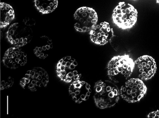
Bud scars on old yeast cells (5 μm bar for scale) — Photo Credit: Ian Foe, (Calico)
Scientists at Calico Life Sciences have pioneered a technique to make targeted perturbations to gene expression in yeast (i.e., allowing them to selectively “turn on” a gene’s activity) with the goal of understanding how aging works at the molecular level. The hope is that understanding aging in yeast will apply to aging in more complex organisms, like humans. This work is an early step in building a predictive framework for understanding the behavior of cells over time.

The Gene Expression Experiment
Genes encoded in DNA only function after being transcribed to RNA. It’s the RNA that is “translated” or “read” by ribosomes to produce protein. The level of protein production is governed by how much RNA is transcribed from DNA. Most of the work in a cell is being done by proteins, so they are key to understanding cell behavior. Yet, while we’d really like to measure the protein production levels, techniques to identify proteins at this scale are prohibitively expensive. Instead, in this experiment we use RNA as a proxy, since measuring RNA levels is easier.

The gene expression experiment is designed to perturb individual genes and measure, over time, how every other gene in the genome responds. The ability to rapidly perturb and track dynamics allows us to learn causal relationships and non-linear behaviors missing in most experiments. These dynamic data can also be used to train predictive models. This is made possible by strains of yeast with a single gene that is responsive to an external switch, in this case the hormone β-estradiol. To perturb a gene, the hormone is introduced, causing the switched gene to be overexpressed by a factor of 50 within 10 minutes. The yeast culture is then sampled at several points in time to measure the gene expression levels on microarrays. These experiments were done in parallel, with one yeast strain per culture, running concurrently.

Most of the perturbation experiments were done on a particular class of genes coding for transcription factors (TFs). These genes are the primary regulators of gene expression, coding for proteins that actually bind to the DNA strands, permitting or blocking transcription of particular genes.

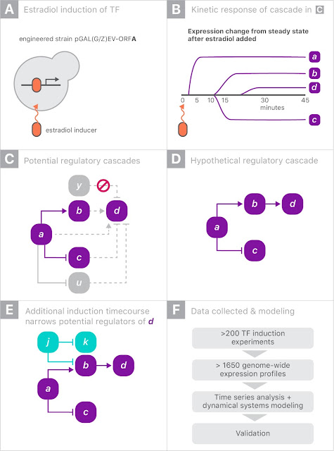
When gene “a” is turned on it may upregulate gene “b” and downregulate gene “c”, and later lead to upregulation of gene “d”. Since yeast has more than 6000 genes, tracing the downstream impact of perturbing a single gene can get complicated very quickly. By combining experiments on different genes, one hopes to disambiguate the exact regulation mechanisms.
Schematic of the genome perturbation experiment: yeast strain with switchable gene “a”. Turning on a single gene (A) can result in differing levels of gene expression over time (B). Tracking these changes in comparison to those induced by turning on other genes (C and D) can provide insight into the regulation mechanisms (E).
The Gene Expression Model
For this experiment, we partnered with Calico because of the scale of the data, and the opportunity to leverage Google’s machine learning expertise and compute resources. There were more than 200 perturbation experiments on different yeast strains, each activating a single gene. In each experiment, the expression levels of all 6000 genes were measured eight times over 90 minutes, yielding a total of almost 20 million individual measurements (panel F, above). Clearly some automation was required to analyze the data.

Our approach was to model the whole process as a system of differential equations: the rate of change of the expression of a gene was proportional to a weighted sum of the expression levels of all genes. We first estimated the time derivatives from the data by simply subtracting the expression levels among adjacent time points. We then predicted the time derivatives using only the raw expression levels themselves. By fitting a linear regression, we are, in effect, fitting the coefficients of a system of differential equations describing gene regulation. Our hope is that the differential equation model would be a low dimensional representation of the data that could be interpreted more easily. To handle overfitting, we regularized the model using the L1-norm, which prefers to set uninformative parameters to exactly zero.

Because each of the 200 experiments was unique, we held out each one in turn, refitting the model and allowing the selection of the best hyperparameters to optimize the out-of-sample loss. In the end, the work required a significant amount of compute, amounting to more than 50 million full regularization paths.

Model Results
Our model made predictions about which genes would code for intermediate regulators of gene expression. This is an attempt at modeling the full gene regulation network of the organism. To verify these predictions, our collaborators at Calico collected more data from ten new strains of yeast. Three out of ten of the predictions held up in these experiments. One of the genes that the model predicted to be active encoded an unverified transcription factor, while another previously identified as a regulator but never followed up, was found by our model to be a very active regulator. Our model was able to identify these without prior biological knowledge, demonstrating that these ML techniques might scale to other domains or organisms that are much less well studied.

More discussion of the impact of this work within the broad context of the field of genomics is available in an independent peer commentary.

Acknowledgements
We wish to thank Marc Coram, Minjie Fan, and Marc Berndl for their foundational contributions to this work, the Google Accelerated Science team for their continual support, and the entire team at Calico for the opportunity to collaborate on this experiment.

Source: Google AI Blog


Seeing More with In Silico Labeling of Microscopy Images


In the fields of biology and medicine, microscopy allows researchers to observe details of cells and molecules which are unavailable to the naked eye. Transmitted light microscopy, where a biological sample is illuminated on one side and imaged, is relatively simple and well-tolerated by living cultures but produces images which can be difficult to properly assess. Fluorescence microscopy, in which biological objects of interest (such as cell nuclei) are specifically targeted with fluorescent molecules, simplifies analysis but requires complex sample preparation. With the increasing application of machine learning to the field of microscopy, including algorithms used to automatically assess the quality of images and assist pathologists diagnosing cancerous tissue, we wondered if we could develop a deep learning system that could combine the benefits of both microscopy techniques while minimizing the downsides.

With “In Silico Labeling: Predicting Fluorescent Labels in Unlabeled Images”, appearing today in Cell, we show that a deep neural network can predict fluorescence images from transmitted light images, generating labeled, useful, images without modifying cells and potentially enabling longitudinal studies in unmodified cells, minimally invasive cell screening for cell therapies, and investigations using large numbers of simultaneous labels. We also open sourced our network, along with the complete training and test data, a trained model checkpoint, and example code.

Background
Transmitted light microscopy techniques are easy to use, but can produce images in which it can be hard to tell what’s going on. An example is the following image from a phase-contrast microscope, in which the intensity of a pixel indicates the degree to which light was phase-shifted as it passed through the sample.
Transmitted light (phase-contrast) image of a human motor neuron culture derived from induced pluripotent stem cells. Outset 1 shows a cluster of cells, possibly neurons. Outset 2 shows a flaw in the image obscuring underlying cells. Outset 3 shows neurites. Outset 4 shows what appear to be dead cells. Scale bar is 40 μm. Source images for this and the following figures come from the Finkbeiner lab at the Gladstone Institutes.
In the above figure, it’s difficult to tell how many cells are in the cluster in Outset 1, or the locations and states of the cells in Outset 4 (hint: there’s a barely-visible flat cell in the upper-middle). It’s also difficult to get fine structures consistently in focus, such as the neurites in Outset 3.

We can get more information out of transmitted light microscopy by acquiring images in z-stacks: sets of images registered in (x, y) where z (the distance from the camera) is systematically varied. This causes different parts of the cells to come in and out of focus, which provides information about a sample’s 3D structure. Unfortunately, it often takes a trained eye to make sense of the z-stack, and analysis of such z-stacks has largely defied automation. An example z-stack is shown below.
A phase-contrast z-stack of the same cells. Note how the appearance changes as the focus is shifted. Now we can see that the fuzzy shape in the lower right of Outset 1 is a single oblong cell, and that the rightmost cell in Outset 4 is taller than the uppermost cell, possibly indicating that it has undergone programmed cell death.
In contrast, fluorescence microscopy images are easier to analyze, because samples are prepared with carefully engineered fluorescent labels which light up just what the researchers want to see. For example, most human cells have exactly one nucleus, so a nuclear label (such as the blue one below) makes it possible for simple tools to find and count cells in an image.
Fluorescence microscopy image of the same cells. The blue fluorescent label localizes to DNA, highlighting cell nuclei. The green fluorescent label localizes to a protein found only in dendrites, a neural substructure. The red fluorescent label localizes to a protein found only in axons, another neural substructure. With these labels it is much easier to understand what’s happening in the sample. For example, the green and red labels in Outset 1 confirm this is a neural cluster. The red label in Outset 3 shows that the neurites are axons, not dendrites. The upper-left blue dot in Outset 4 reveals a previously hard-to-see nucleus, and the lack of a blue dot for the cell at the left shows it to be DNA-free cellular debris.
However, fluorescence microscopy can have significant downsides. First, there is the complexity and variability introduced by the sample preparation and fluorescent labels themselves. Second, when there are many different fluorescent labels in a sample, spectral overlap can make it hard to tell which color belongs to which label, typically limiting researchers to three or four simultaneous labels in a sample. Third, fluorescence labeling may be toxic to cells and sometimes involves protocols that outright kill them, which makes labeling difficult to use in longitudinal studies where the same cells are followed through time.

Seeing more with deep learning
In our paper, we show that a deep neural network can predict fluorescence images from transmitted light z-stacks. To do this, we created a dataset of transmitted light z-stacks matched to fluorescence images and trained a neural network to predict the fluorescence images from the z-stacks. The following diagram explains the process.
Overview of our system. (A) The dataset of training examples: pairs of transmitted light images from z-stacks with pixel-registered sets of fluorescence images of the same scene. Several different fluorescent labels were used to generate fluorescence images and were varied between training examples; the checkerboard images indicate fluorescent labels which were not acquired for a given example. (B) The untrained deep network was (C) trained on the data A. (D) A z-stack of images of a novel scene. (E) The trained network, C, is used to predict fluorescence labels learned from A for each pixel in the novel images, D.
In the course of this work we developed a new neural network composed of three kinds of basic building-blocks, inspired by the modular design of Inception: an in-scale configuration which does not change the spatial scaling of the features, a down-scale configuration which doubles the spatial scaling, and an up-scale configuration which halves it. This lets us break the hard problem of network architecture design into two easier problems: the arrangement of the building-blocks (macro-architecture), and the design of the building-blocks themselves (micro-architecture). We solved the first problem using design principles discussed in the paper, and the second via an automated search powered by Google Hypertune.

To make sure our method was sound, we validated our model using data from an Alphabet lab as well as two external partners: Steve Finkbeiner's lab at the Gladstone Institutes, and the Rubin Lab at Harvard. These data spanned three transmitted light imaging modalities (bright-field, phase-contrast, and differential interference contrast) and three culture types (human motor neurons derived from induced pluripotent stem cells, rat cortical cultures, and human breast cancer cells). We found that our method can accurately predict several labels including those for nuclei, cell type (e.g. neural), and cell state (e.g. cell death). The following figure shows the model’s predictions alongside the transmitted light input and fluorescence ground-truth for our motor neuron example.
Animation showing the same cells in transmitted light and fluorescence imaging, along with predicted fluorescence labels from our model. Outset 2 shows the model predicts the correct labels despite the artifact in the input image. Outset 3 shows the model infers these processes are axons, possibly because of their distance from the nearest cells. Outset 4 shows the model sees the hard-to-see cell at the top, and correctly identifies the object at the left as DNA-free cell debris.
Try it for yourself!
We’ve open sourced our model, along with our full dataset, code for training and inference, and an example. We’re pleased to report that new labels can be learned with minimal additional training data: in the paper and example code, we show a new label may be learned from a single image. This is due to a phenomenon called transfer learning, where a model can learn a new task more quickly and using less training data if it has already mastered similar tasks.

We hope the ability to generate labeled, useful, images without modifying cells will open up completely new kinds of experiments in biology and medicine. If you’re excited to try this technology in your own work, please read the paper or check out the code!

Acknowledgements
We thank the Google Accelerated Science team for originating and developing this project and its publication, and additionally Kevin P. Murphy for supporting its publication. We thank Mike Ando, Youness Bennani, Amy Chung-Yu Chou, Jason Freidenfelds, Jason Miller, Kevin P. Murphy, Philip Nelson, Patrick Riley, and Samuel Yang for ideas and editing help with this post. This study was supported by NINDS (NS091046, NS083390, NS101995), the NIH’s National Institute on Aging (AG065151, AG058476), the NIH’s National Human Genome Research Institute (HG008105), Google, the ALS Association, and the Michael J. Fox Foundation.

Source: Google AI Blog


Using Deep Learning to Facilitate Scientific Image Analysis


Many scientific imaging applications, especially microscopy, can produce terabytes of data per day. These applications can benefit from recent advances in computer vision and deep learning. In our work with biologists on robotic microscopy applications (e.g., to distinguish cellular phenotypes) we've learned that assembling high quality image datasets that separate signal from noise is a difficult but important task. We've also learned that there are many scientists who may not write code, but who are still excited to utilize deep learning in their image analysis work. A particular challenge we can help address involves dealing with out-of-focus images. Even with the autofocus systems on state-of-the-art microscopes, poor configuration or hardware incompatibility may result in image quality issues. Having an automated way to rate focus quality can enable the detection, troubleshooting and removal of such images.

Deep Learning to the Rescue
In “Assessing Microscope Image Focus Quality with Deep Learning”, we trained a deep neural network to rate the focus quality of microscopy images with higher accuracy than previous methods. We also integrated the pre-trained TensorFlow model with plugins in Fiji (ImageJ) and CellProfiler, two leading open source scientific image analysis tools that can be used with either a graphical user interface or invoked via scripts.
A pre-trained TensorFlow model rates focus quality for a montage of microscope image patches of cells in Fiji (ImageJ). Hue and lightness of the borders denote predicted focus quality and prediction uncertainty, respectively.
Our publication and source code (TensorFlow, Fiji, CellProfiler) illustrate the basics of a machine learning project workflow: assembling a training dataset (we synthetically defocused 384 in-focus images of cells, avoiding the need for a hand-labeled dataset), training a model using data augmentation, evaluating generalization (in our case, on unseen cell types acquired by an additional microscope) and deploying the pre-trained model. Previous tools for identifying image focus quality often require a user to manually review images for each dataset to determine a threshold between in and out-of-focus images; our pre-trained model requires no user set parameters to use, and can rate focus quality more accurately as well. To help improve interpretability, our model evaluates focus quality on 84×84 pixel patches which can be visualized with colored patch borders.

What about Images without Objects?
An interesting challenge we overcame was that there are often "blank" image patches with no objects, a scenario where no notion of focus quality exists. Instead of explicitly labeling these "blank" patches and teaching our model to recognize them as a separate category, we configured our model to predict a probability distribution across defocus levels, allowing it to learn to express uncertainty (dim borders in the figure) for these empty patches (e.g. predict equal probability in/out-of-focus).

What's Next?
Deep learning-based approaches for scientific image analysis will improve accuracy, reduce manual parameter tuning and may reveal new insights. Clearly, the sharing and availability of datasets and models, and implementation into tools that are proven to be useful within respective communities, will be important for widespread adoption.

Acknowledgements
We thank Claire McQuin, Allen Goodman, Anne Carpenter of the Broad Institute and Kevin Eliceiri of the University of Wisconsin at Madison for assistance with CellProfiler and Fiji integration, respectively.

Source: Google AI Blog


So there I was, firing a megawatt plasma collider at work…


Wait, what? Why is Google interested in plasma physics?

Google is always interested in solving complex engineering problems, and few are more complex than fusion. Physicists have been trying since the 1950s to control the fusion of hydrogen atoms into helium, which is the same process that powers the Sun. The key to harnessing this power is to confine hydrogen plasmas for long enough to get more energy out from fusion reactions than was put in. This point is called “breakeven.” If it works, it would represent a technological breakthrough, and could provide an abundant source of zero-carbon energy.

There are currently several large academic and government research efforts in fusion. Just to rattle off a few, in plasma fusion there are tokamak machines like ITER and stellarator machines like Wendelstein 7-X. The stellarator design actually goes back to 1951, so physicists have been working on this for a while. Oh yeah, and if you like giant lasers, there’s the National Ignition Facility which users lasers to generate X-rays to generate fusion reactions. So far, none of these has gotten to the economic breakeven point.

All of these efforts involve complex experiments with many variables, providing an opportunity for Google to help, with our strength in computing and machine learning. Today, we’re publishing “Achievement of Sustained Net Plasma Heating in a Fusion Experiment with the Optometrist Algorithm” in Scientific Reports. This paper describes the first results of Google’s collaboration with the physicists and engineers at Tri Alpha Energy, taking a step towards the breakeven goal.

Did you really just say that you got to fire a plasma collider?

Yeah. Tri Alpha Energy has a unique scheme for plasma confinement called a field-reversed configuration that’s predicted to get more stable as the energy goes up, in contrast to other methods where plasmas get harder to control as you heat them. Tri Alpha built a giant ionized plasma machine, C-2U, that fills an entire warehouse in an otherwise unassuming office park. The plasma that this machine generates and confines exhibits all kinds of highly nonlinear behavior. The machine itself pushes the envelope of how much electrical power can be applied to generate and confine the plasma in such a small space over such a short time. It’s a complex machine with more than 1000 knobs and switches, an investment (not ours!) in exploring clean energy north of $100 million. This is a high-stakes optimization problem, dealing with both plasma performance and equipment constraints. This is where Google comes in.
End-on view of C-2U
Wait, why not just simulate what will happen? Isn’t this simple physics?

The “simple” simulations using magnetohydrodynamics don’t really apply. Even if these machines operated in that limit, which they very much don’t, the simulations make fluid dynamics simulations look easy! The reality is much more complicated, as the ion temperature is three times larger than the electron temperature, so the plasma is far out of thermal equilibrium, also, the fluid approximation is totally invalid, so you have to track at least some of the trillion+ individual particles, so the whole thing is beyond what we know how to do even with Google-scale compute resources.

So why are we doing this? Real experiments! With atoms not bits! At Google we love to run experiments and optimize things. We thought it would be a great challenge to see if we could help Tri Alpha. They run a plasma “shot” on the C-2U machine every 8 minutes. Each shot consists of creating two spinning blobs of plasma in the vacuum sealed innards of C-2U, smashing them together at over 600,000 miles per hour, creating a bigger, hotter, spinning football of plasma. Then they blast it continuously with particle beams (actually neutral hydrogen atoms) to keep it spinning. They hang on to the spinning football with magnetic fields for as long as 10 milliseconds. They’re trying to experimentally verify that these advanced beam driven field-reversed plasma configurations behave as expected by theory. If they do, this scheme could lead to net-energy-out fusion.

Now 8 minutes sounds like a long time (which is the time it takes for C-2U to cool, recharge, and get ready for another 10 ms shot), but when you’re sitting in the control room during an experimental campaign, it goes by really quickly. There are a lot of sensor outputs to look at, to try to figure out how the plasma was behaving. Before you know it, the power supplies are charged again, and they’re ready for another go!

What was that about optimization? What are you optimizing?

That’s the thing, it’s not completely obvious what good plasma performance is. Of course, Tri Alpha has some of the world’s best plasma physicists, but even they disagree on what “good” is. We can boil down the machine controls to “only” 30 parameters or so, but when you have to wait 8 minutes per experiment, it’s a pretty hard problem even with a concrete objective. Also, it’s not entirely known, day-to-day, what the reliable operating envelope of the machine is. And it keeps changing since the quality of the vacuum keeps changing and electrodes wear out and...

So we boil the problem down to “let’s find plasma behaviors that an expert human plasma physicist thinks are interesting, and let’s not break the machine when we’re doing it.” We developed the Optometrist Algorithm, which is sort of a Markov Chain Monte Carlo (MCMC) where the likelihood function being explored is in the plasma physicist’s mind rather than being explicitly written down. Just like getting an eyeglass prescription, the algorithm presents the expert human with machine settings and the associated outcomes. They can just use their judgement on what is interesting, and what is unhealthy for the machine. These could be “That initial collision looked really strong!” or “The edge biasing is actually working well now!” or “Wow, that was awesome, but the electrode current was way too high, let’s not do that again!” The key improvement we provided was a technique to search the high-dimensional space of machine parameters efficiently.

Oh, I like MCMC, it’s like the best thing ever!

I knew you’d like that bit. Using this technique, we actually found something really interesting. As we describe in our paper, we found a regime where the neutral particle beams dumping energy into the plasma were able to completely balance the cooling losses, and the total energy in the plasma actually went up after formation. It was only for about 2 milliseconds, but still, it was a first! Since rising energy due to neutral beam heating was not necessarily expected for C-2U, it would have been difficult to plug into an objective function. We really needed a human expert to notice. This was a classic case of humans and computers doing a better job together than either could have separately. You know how it is — when you think you have an optimization problem, and you optimize the objective, you usually just look at the result and say, “No no no, that’s not what I meant,” and you add some other term and repeat until you get sick of it?

That hasn’t happened to me. This week. Yet.

Yeah, so we just cut out that iteration and let the expert human use their judgment. This learning from human preferences is becoming a thing. Google and Tri Alpha made a pretty good team for it, for a really important problem.

So what now?

So actually, Tri Alpha learned everything they could have from C-2U and then dismantled it. They built a new machine called Norman (after their late co-founder Norman Rostoker) in the same warehouse. It’s much more powerful both in plasma acceleration and in neutral particle beams. It also has a more sophisticated system to confine the plasma in the central region. The pressure vessel, accelerators, and banks of capacitors and power supplies cover the building’s concrete floor.
They just achieved “first plasma” on it. They’re hoping, with our help, to verify this theoretical prediction that the plasma will actually behave better in the “burning plasma” regime. If they can do that over the next 18 months, it will be a lot more likely that the field-reversed configuration is a viable approach for breakeven fusion. In that case, Tri Alpha will try to build their follow-on design, an actual demonstration power generator. That one won’t fit in their warehouse!

Acknowledgements
On the Google side, we wish to thank John Platt, Michael Dikovsky, Patrick Riley and Ross Koningstein for their significant contributions to this work. We thank the Google Accelerated Science team for their continual support. We are also grateful to the entire team at Tri Alpha for giving us the opportunity to try our hand at optimization for this crucially important problem.