Tag Archives: #AutoML

LayerNAS: Neural Architecture Search in Polynomial Complexity

Every byte and every operation matters when trying to build a faster model, especially if the model is to run on-device. Neural architecture search (NAS) algorithms design sophisticated model architectures by searching through a larger model-space than what is possible manually. Different NAS algorithms, such as MNasNet and TuNAS, have been proposed and have discovered several efficient model architectures, including MobileNetV3, EfficientNet.

Here we present LayerNAS, an approach that reformulates the multi-objective NAS problem within the framework of combinatorial optimization to greatly reduce the complexity, which results in an order of magnitude reduction in the number of model candidates that must be searched, less computation required for multi-trial searches, and the discovery of model architectures that perform better overall. Using a search space built on backbones taken from MobileNetV2 and MobileNetV3, we find models with top-1 accuracy on ImageNet up to 4.9% better than current state-of-the-art alternatives.


Problem formulation

NAS tackles a variety of different problems on different search spaces. To understand what LayerNAS is solving, let's start with a simple example: You are the owner of GBurger and are designing the flagship burger, which is made up with three layers, each of which has four options with different costs. Burgers taste differently with different mixtures of options. You want to make the most delicious burger you can that comes in under a certain budget.

Make up your burger with different options available for each layer, each of which has different costs and provides different benefits.

Just like the architecture for a neural network, the search space for the perfect burger follows a layerwise pattern, where each layer has several options with different changes to costs and performance. This simplified model illustrates a common approach for setting up search spaces. For example, for models based on convolutional neural networks (CNNs), like MobileNet, the NAS algorithm can select between a different number of options — filters, strides, or kernel sizes, etc. — for the convolution layer.


Method

We base our approach on search spaces that satisfy two conditions:

  • An optimal model can be constructed using one of the model candidates generated from searching the previous layer and applying those search options to the current layer.
  • If we set a FLOP constraint on the current layer, we can set constraints on the previous layer by reducing the FLOPs of the current layer.

Under these conditions it is possible to search linearly, from layer 1 to layer n knowing that when searching for the best option for layer i, a change in any previous layer will not improve the performance of the model. We can then bucket candidates by their cost, so that only a limited number of candidates are stored per layer. If two models have the same FLOPs, but one has better accuracy, we only keep the better one, and assume this won’t affect the architecture of following layers. Whereas the search space of a full treatment would expand exponentially with layers since the full range of options are available at each layer, our layerwise cost-based approach allows us to significantly reduce the search space, while being able to rigorously reason over the polynomial complexity of the algorithm. Our experimental evaluation shows that within these constraints we are able to discover top-performance models.


NAS as a combinatorial optimization problem

By applying a layerwise-cost approach, we reduce NAS to a combinatorial optimization problem. I.e., for layer i, we can compute the cost and reward after training with a given component Si . This implies the following combinatorial problem: How can we get the best reward if we select one choice per layer within a cost budget? This problem can be solved with many different methods, one of the most straightforward of which is to use dynamic programming, as described in the following pseudo code:

while True:
	# select a candidate to search in Layer i
	candidate = select_candidate(layeri)
	if searchable(candidate):
		# Use the layerwise structural information to generate the children.
		children = generate_children(candidate)
		reward = train(children)
		bucket = bucketize(children)
		if memorial_table[i][bucket] < reward:
			memorial_table[i][bucket] = children
		move to next layer
Pseudocode of LayerNAS.
Illustration of the LayerNAS approach for the example of trying to create the best burger within a budget of $7–$9. We have four options for the first layer, which results in four burger candidates. By applying four options on the second layer, we have 16 candidates in total. We then bucket them into ranges from $1–$2, $3–$4, $5–$6, and $7–$8, and only keep the most delicious burger within each of the buckets, i.e., four candidates. Then, for those four candidates, we build 16 candidates using the pre-selected options for the first two layers and four options for each candidate for the third layer. We bucket them again, select the burgers within the budget range, and keep the best one.

Experimental results

When comparing NAS algorithms, we evaluate the following metrics:

  • Quality: What is the most accurate model that the algorithm can find?
  • Stability: How stable is the selection of a good model? Can high-accuracy models be consistently discovered in consecutive trials of the algorithm?
  • Efficiency: How long does it take for the algorithm to find a high-accuracy model?

We evaluate our algorithm on the standard benchmark NATS-Bench using 100 NAS runs, and we compare against other NAS algorithms, previously described in the NATS-Bench paper: random search, regularized evolution, and proximal policy optimization. Below, we visualize the differences between these search algorithms for the metrics described above. For each comparison, we record the average accuracy and variation in accuracy (variation is noted by a shaded region corresponding to the 25% to 75% interquartile range).

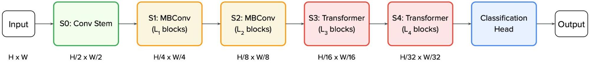
NATS-Bench size search defines a 5-layer CNN model, where each layer can choose from eight different options, each with different channels on the convolution layers. Our goal is to find the best model with 50% of the FLOPs required by the largest model. LayerNAS performance stands apart because it formulates the problem in a different way, separating the cost and reward to avoid searching a significant number of irrelevant model architectures. We found that model candidates with fewer channels in earlier layers tend to yield better performance, which explains how LayerNAS discovers better models much faster than other algorithms, as it avoids spending time on models outside the desired cost range. Note that the accuracy curve drops slightly after searching longer due to the lack of correlation between validation accuracy and test accuracy, i.e., some model architectures with higher validation accuracy have a lower test accuracy in NATS-Bench size search.

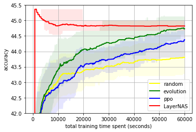
Top: NATS-Bench size search test accuracy on Cifar10; Middle: On Cifar100; Bottom: On ImageNet16-120. Average on 100 runs compared with random search (random), Regularized Evolution (evolution), and Proximal Policy Optimization (PPO).

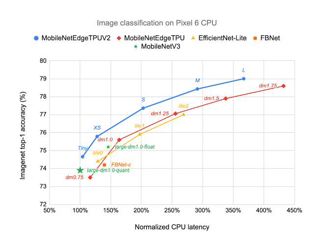
We construct search spaces based on MobileNetV2, MobileNetV2 1.4x, MobileNetV3 Small, and MobileNetV3 Large and search for an optimal model architecture under different #MADDs (number of multiply-additions per image) constraints. Among all settings, LayerNAS finds a model with better accuracy on ImageNet. See the paper for details.

Comparison on models under different #MAdds.

Conclusion

In this post, we demonstrated how to reformulate NAS into a combinatorial optimization problem, and proposed LayerNAS as a solution that requires only polynomial search complexity. We compared LayerNAS with existing popular NAS algorithms and showed that it can find improved models on NATS-Bench. We also use the method to find better architectures based on MobileNetV2, and MobileNetV3.


Acknowledgements

We would like to thank Jingyue Shen, Keshav Kumar, Daiyi Peng, Mingxing Tan, Esteban Real, Peter Young, Weijun Wang, Qifei Wang, Xuanyi Dong, Xin Wang, Yingjie Miao, Yun Long, Zhuo Wang, Da-Cheng Juan, Deqiang Chen, Fotis Iliopoulos, Han-Byul Kim, Rino Lee, Andrew Howard, Erik Vee, Rina Panigrahy, Ravi Kumar and Andrew Tomkins for their contribution, collaboration and advice.

Source: Google AI Blog


Open Source Vizier: Towards reliable and flexible hyperparameter and blackbox optimization

Google Vizier is the de-facto system for blackbox optimization over objective functions and hyperparameters across Google, having serviced some of Google’s largest research efforts and optimized a wide range of products (e.g., Search, Ads, YouTube). For research, it has not only reduced language model latency for users, designed computer architectures, accelerated hardware, assisted protein discovery, and enhanced robotics, but also provided a reliable backend interface for users to search for neural architectures and evolve reinforcement learning algorithms. To operate at the scale of optimizing thousands of users’ critical systems and tuning millions of machine learning models, Google Vizier solved key design challenges in supporting diverse use cases and workflows, while remaining strongly fault-tolerant.

Today we are excited to announce Open Source (OSS) Vizier (with an accompanying systems whitepaper published at AutoML Conference 2022), a standalone Python package based on Google Vizier. OSS Vizier is designed for two main purposes: (1) managing and optimizing experiments at scale in a reliable and distributed manner for users, and (2) developing and benchmarking algorithms for automated machine learning (AutoML) researchers.


System design

OSS Vizier works by having a server provide services, namely the optimization of blackbox objectives, or functions, from multiple clients. In the main workflow, a client sends a remote procedure call (RPC) and asks for a suggestion (i.e., a proposed input for the client’s blackbox function), from which the service begins to spawn a worker to launch an algorithm (i.e., a Pythia policy) to compute the following suggestions. The suggestions are then evaluated by clients to form their corresponding objective values and measurements, which are sent back to the service. This pipeline is repeated multiple times to form an entire tuning trajectory.

The use of the ubiquitous gRPC library, which is compatible with most programming languages, such as C++ and Rust, allows maximum flexibility and customization, where the user can also write their own custom clients and even algorithms outside of the default Python interface. Since the entire process is saved to an SQL datastore, a smooth recovery is ensured after a crash, and usage patterns can be stored as valuable datasets for research into meta-learning and multitask transfer-learning methods such as the OptFormer and HyperBO.

In the distributed pipeline, multiple clients each send a “Suggest” request to the Service API, which produces Suggestions for the clients using Pythia. The clients evaluate these suggestions and return measurements. All transactions are stored to allow fault-tolerance.

Usage

Because of OSS Vizier’s emphasis as a service, in which clients can send requests to the server at any point in time, it is thus designed for a broad range of scenarios — the budget of evaluations, or trials, can range from tens to millions, and the evaluation latency can range from seconds to weeks. Evaluations can be done asynchronously (e.g., tuning an ML model) or in synchronous batches (e.g., wet lab settings involving multiple simultaneous experiments). Furthermore, evaluations may fail due to transient errors and be retried, or may fail due to persistent errors (e.g., the evaluation is impossible) and should not be retried.

This broadly supports a variety of applications, which include hyperparameter tuning deep learning models or optimizing non-computational objectives, which can be e.g., physical, chemical, biological, mechanical, or even human-evaluated, such as cookie recipes.

The OSS Vizier API allows (1) developers to integrate other packages, with PyGlove and Vertex Vizier already included, and (2) users to optimize their experiments, such as machine learning pipelines and cookie recipes.

Integrations, algorithms, and benchmarks

As Google Vizier is heavily integrated with many of Google’s internal frameworks and products, OSS Vizier will naturally be heavily integrated with many of Google’s open source and external frameworks. Most prominently, OSS Vizier will serve as a distributed backend for PyGlove to allow large-scale evolutionary searches over combinatorial primitives such as neural architectures and reinforcement learning algorithms. Furthermore, OSS Vizier shares the same client-based API with Vertex Vizier, allowing users to quickly swap between open-source and production-quality services.

For AutoML researchers, OSS Vizier is also outfitted with a useful collection of algorithms and benchmarks (i.e., objective functions) unified under common APIs for assessing the strengths and weaknesses of proposed methods. Most notably, via TensorFlow Probability, researchers can now use the JAX-based Gaussian Process Bandit algorithm, based on the default algorithm in Google Vizier that tunes internal users’ objectives.


Resources and future direction

We provide links to the codebase, documentation, and systems whitepaper. We plan to allow user contributions, especially in the form of algorithms and benchmarks, and further integrate with the open-source AutoML ecosystem. Going forward, we hope to see OSS Vizier as a core tool for expanding research and development over blackbox optimization and hyperparameter tuning.


Acknowledgements

OSS Vizier was developed by members of the Google Vizier team in collaboration with the TensorFlow Probability team: Setareh Ariafar, Lior Belenki, Emily Fertig, Daniel Golovin, Tzu-Kuo Huang, Greg Kochanski, Chansoo Lee, Sagi Perel, Adrian Reyes, Xingyou (Richard) Song, and Richard Zhang.

In addition, we thank Srinivas Vasudevan, Jacob Burnim, Brian Patton, Ben Lee, Christopher Suter, and Rif A. Saurous for further TensorFlow Probability integrations, Daiyi Peng and Yifeng Lu for PyGlove integrations, Hao Li for Vertex/Cloud integrations, Yingjie Miao for AutoRL integrations, Tom Hennigan, Varun Godbole, Pavel Sountsov, Alexey Volkov, Mihir Paradkar, Richard Belleville, Bu Su Kim, Vytenis Sakenas, Yujin Tang, Yingtao Tian, and Yutian Chen for open source and infrastructure help, and George Dahl, Aleksandra Faust, Claire Cui, and Zoubin Ghahramani for discussions.

Finally we thank Tom Small for designing the animation for this post.

Source: Google AI Blog


OptFormer: Towards Universal Hyperparameter Optimization with Transformers

One of the most important aspects in machine learning is hyperparameter optimization, as finding the right hyperparameters for a machine learning task can make or break a model’s performance. Internally, we regularly use Google Vizier as the default platform for hyperparameter optimization. Throughout its deployment over the last 5 years, Google Vizier has been used more than 10 million times, over a vast class of applications, including machine learning applications from vision, reinforcement learning, and language but also scientific applications such as protein discovery and hardware acceleration. As Google Vizier is able to keep track of use patterns in its database, such data, usually consisting of optimization trajectories termed studies, contain very valuable prior information on realistic hyperparameter tuning objectives, and are thus highly attractive for developing better algorithms.

While there have been many previous methods for meta-learning over such data, such methods share one major common drawback: their meta-learning procedures depend heavily on numerical constraints such as the number of hyperparameters and their value ranges, and thus require all tasks to use the exact same total hyperparameter search space (i.e., tuning specifications). Additional textual information in the study, such as its description and parameter names, are also rarely used, yet can hold meaningful information about the type of task being optimized. Such a drawback becomes more exacerbated for larger datasets, which often contain significant amounts of such meaningful information.

Today in “Towards Learning Universal Hyperparameter Optimizers with Transformers”, we are excited to introduce the OptFormer, one of the first Transformer-based frameworks for hyperparameter tuning, learned from large-scale optimization data using flexible text-based representations. While numerous works have previously demonstrated the Transformer’s strong abilities across various domains, few have touched on its optimization-based capabilities, especially over text space. Our core findings demonstrate for the first time some intriguing algorithmic abilities of Transformers: 1) a single Transformer network is capable of imitating highly complex behaviors from multiple algorithms over long horizons; 2) the network is further capable of predicting objective values very accurately, in many cases surpassing Gaussian Processes, which are commonly used in algorithms such as Bayesian Optimization.

Approach: Representing Studies as Tokens
Rather than only using numerical data as common with previous methods, our novel approach instead utilizes concepts from natural language and represents all of the study data as a sequence of tokens, including textual information from initial metadata. In the animation below, this includes “CIFAR10”, “learning rate”, “optimizer type”, and “Accuracy”, which informs the OptFormer of an image classification task. The OptFormer then generates new hyperparameters to try on the task, predicts the task accuracy, and finally receives the true accuracy, which will be used to generate the next round’s hyperparameters. Using the T5X codebase, the OptFormer is trained in a typical encoder-decoder fashion using standard generative pretraining over a wide range of hyperparameter optimization objectives, including real world data collected by Google Vizier, as well as public hyperparameter (HPO-B) and blackbox optimization benchmarks (BBOB).

The OptFormer can perform hyperparameter optimization encoder-decoder style, using token-based representations. It initially observes text-based metadata (in the gray box) containing information such as the title, search space parameter names, and metrics to optimize, and repeatedly outputs parameter and objective value predictions.

Imitating Policies
As the OptFormer is trained over optimization trajectories by various algorithms, it may now accurately imitate such algorithms simultaneously. By providing a text-based prompt in the metadata for the designated algorithm (e.g. “Regularized Evolution”), the OptFormer will imitate the algorithm’s behavior.

Over an unseen test function, the OptFormer produces nearly identical optimization curves as the original algorithm. Mean and standard deviation error bars are shown.

Predicting Objective Values
In addition, the OptFormer may now predict the objective value being optimized (e.g. accuracy) and provide uncertainty estimates. We compared the OptFormer’s prediction with a standard Gaussian Process and found that the OptFormer was able to make significantly more accurate predictions. This can be seen below qualitatively, where the OptFormer’s calibration curve closely follows the ideal diagonal line in a goodness-of-fit test, and quantitatively through standard aggregate metrics such as log predictive density.

Left: Rosenblatt Goodness-of-Fit. Closer diagonal fit is better. Right: Log Predictive Density. Higher is better.

Combining Both: Model-based Optimization
We may now use the OptFormer’s function prediction capability to better guide our imitated policy, similar to techniques found in Bayesian Optimization. Using Thompson Sampling, we may rank our imitated policy’s suggestions and only select the best according to the function predictor. This produces an augmented policy capable of outperforming our industry-grade Bayesian Optimization algorithm in Google Vizier when optimizing classic synthetic benchmark objectives and tuning the learning rate hyperparameters of a standard CIFAR-10 training pipeline.

Left: Best-so-far optimization curve over a classic Rosenbrock function. Right: Best-so-far optimization curve over hyperparameters for training a ResNet-50 on CIFAR-10 via init2winit. Both cases use 10 seeds per curve, and error bars at 25th and 75th percentiles.

Conclusion
Throughout this work, we discovered some useful and previously unknown optimization capabilities of the Transformer. In the future, we hope to pave the way for a universal hyperparameter and blackbox optimization interface to use both numerical and textual data to facilitate optimization over complex search spaces, and integrate the OptFormer with the rest of the Transformer ecosystem (e.g. language, vision, code) by leveraging Google’s vast collection of offline AutoML data.

Acknowledgements
The following members of DeepMind and the Google Research Brain Team conducted this research: Yutian Chen, Xingyou Song, Chansoo Lee, Zi Wang, Qiuyi Zhang, David Dohan, Kazuya Kawakami, Greg Kochanski, Arnaud Doucet, Marc'aurelio Ranzato, Sagi Perel, and Nando de Freitas.

We would like to also thank Chris Dyer, Luke Metz, Kevin Murphy, Yannis Assael, Frank Hutter, and Esteban Real for providing valuable feedback, and further thank Sebastian Pineda Arango, Christof Angermueller, and Zachary Nado for technical discussions on benchmarks. In addition, we thank Daniel Golovin, Daiyi Peng, Yingjie Miao, Jack Parker-Holder, Jie Tan, Lucio Dery, and Aleksandra Faust for multiple useful conversations.

Finally, we thank Tom Small for designing the animation for this post.

Source: Google AI Blog


Building Efficient Multiple Visual Domain Models with Multi-path Neural Architecture Search

Deep learning models for visual tasks (e.g., image classification) are usually trained end-to-end with data from a single visual domain (e.g., natural images or computer generated images). Typically, an application that completes visual tasks for multiple domains would need to build multiple models for each individual domain, train them independently (meaning no data is shared between domains), and then at inference time each model would process domain-specific input data. However, early layers between these models generate similar features, even for different domains, so it can be more efficient — decreasing latency and power consumption, lower memory overhead to store parameters of each model — to jointly train multiple domains, an approach referred to as multi-domain learning (MDL). Moreover, an MDL model can also outperform single domain models due to positive knowledge transfer, which is when additional training on one domain actually improves performance for another. The opposite, negative knowledge transfer, can also occur, depending on the approach and specific combination of domains involved. While previous work on MDL has proven the effectiveness of jointly learning tasks across multiple domains, it involved a hand-crafted model architecture that is inefficient to apply to other work.

In “Multi-path Neural Networks for On-device Multi-domain Visual Classification”, we propose a general MDL model that can: 1) achieve high accuracy efficiently (keeping the number of parameters and FLOPS low), 2) learn to enhance positive knowledge transfer while mitigating negative transfer, and 3) effectively optimize the joint model while handling various domain-specific difficulties. As such, we propose a multi-path neural architecture search (MPNAS) approach to build a unified model with heterogeneous network architecture for multiple domains. MPNAS extends the efficient neural architecture search (NAS) approach from single path search to multi-path search by finding an optimal path for each domain jointly. Also, we introduce a new loss function, called adaptive balanced domain prioritization (ABDP) that adapts to domain-specific difficulties to help train the model efficiently. The resulting MPNAS approach is efficient and scalable; the resulting model maintains performance while reducing the model size and FLOPS by 78% and 32%, respectively, compared to a single-domain approach.

Multi-Path Neural Architecture Search
To encourage positive knowledge transfer and avoid negative transfer, traditional solutions build an MDL model so that domains share most of the layers that learn the shared features across domains (called feature extraction), then have a few domain-specific layers on top. However, such a homogenous approach to feature extraction cannot handle domains with significantly different features (e.g., objects in natural images and art paintings). On the other hand, handcrafting a unified heterogeneous architecture for each MDL model is time-consuming and requires domain-specific knowledge.

NAS is a powerful paradigm for automatically designing deep learning architectures. It defines a search space, made up of various potential building blocks that could be part of the final model. The search algorithm finds the best candidate architecture from the search space that optimizes the model objectives, e.g., classification accuracy. Recent NAS approaches (e.g., TuNAS) have meaningfully improved search efficiency by using end-to-end path sampling, which enables us to scale NAS from single domains to MDL.

Inspired by TuNAS, MPNAS builds the MDL model architecture in two stages: search and training. In the search stage, to find an optimal path for each domain jointly, MPNAS creates an individual reinforcement learning (RL) controller for each domain, which samples an end-to-end path (from input layer to output layer) from the supernetwork (i.e., the superset of all the possible subnetworks between the candidate nodes defined by the search space). Over multiple iterations, all the RL controllers update the path to optimize the RL rewards across all domains. At the end of the search stage, we obtain a subnetwork for each domain. Finally, all the subnetworks are combined to build a heterogeneous architecture for the MDL model, shown below.

Since the subnetwork for each domain is searched independently, the building block in each layer can be shared by multiple domains (i.e., dark gray nodes), used by a single domain (i.e., light gray nodes), or not used by any subnetwork (i.e., dotted nodes). The path for each domain can also skip any layer during search. Given the subnetwork can freely select which blocks to use along the path in a way that optimizes performance (rather than, e.g., arbitrarily designating which layers are homogenous and which are domain-specific), the output network is both heterogeneous and efficient.

Example architecture searched by MPNAS. Dashed paths represent all the possible subnetworks. Solid paths represent the selected subnetworks for each domain (highlighted in different colors). Nodes in each layer represent the candidate building blocks defined by the search space.

The figure below demonstrates the searched architecture of two visual domains among the ten domains of the Visual Domain Decathlon challenge. One can see that the subnetwork of these two highly related domains (one red, the other green) share a majority of building blocks from their overlapping paths, but there are still some differences.

Architecture blocks of two domains (ImageNet and Describable Textures) among the ten domains of the Visual Domain Decathlon challenge. Red and green path represents the subnetwork of ImageNet and Describable Textures, respectively. Dark pink nodes represent the blocks shared by multiple domains. Light pink nodes represent the blocks used by each path. The model is built based on MobileNet V3-like search space. The “dwb” block in the figure represents the dwbottleneck block. The “zero” block in the figure indicates the subnetwork skips that block.

Below we show the path similarity between domains among the ten domains of the Visual Domain Decathlon challenge. The similarity is measured by the Jaccard similarity score between the subnetworks of each domain, where higher means the paths are more similar. As one might expect, domains that are more similar share more nodes in the paths generated by MPNAS, which is also a signal of strong positive knowledge transfer. For example, the paths for similar domains (like ImageNet, CIFAR-100, and VGG Flower, which all include objects in natural images) have high scores, while the paths for dissimilar domains (like Daimler Pedestrian Classification and UCF101 Dynamic Images, which include pedestrians in grayscale images and human activity in natural color images, respectively) have low scores.

Confusion matrix for the Jaccard similarity score between the paths for the ten domains. Score value ranges from 0 to 1. A greater value indicates two paths share more nodes.

Training a Heterogeneous Multi-domain Model
In the second stage, the model resulting from MPNAS is trained from scratch for all domains. For this to work, it is necessary to define a unified objective function for all the domains. To successfully handle a large variety of domains, we designed an algorithm that adapts throughout the learning process such that losses are balanced across domains, called adaptive balanced domain prioritization (ABDP).

Below we show the accuracy, model size, and FLOPS of the model trained in different settings. We compare MPNAS to three other approaches:

  • Domain independent NAS: Searching and training a model for each domain separately.
  • Single path multi-head: Using a pre-trained model as a shared backbone for all domains with separated classification heads for each domain.
  • Multi-head NAS: Searching a unified backbone architecture for all domains with separated classification heads for each domain.

From the results, we can observe that domain independent NAS requires building a bundle of models for each domain, resulting in a large model size. Although single path multi-head and multi-head NAS can reduce the model size and FLOPS significantly, forcing the domains to share the same backbone introduces negative knowledge transfer, decreasing overall accuracy.

Model   Number of parameters ratio     GFLOPS     Average Top-1 accuracy  
Domain independent NAS     5.7x 1.08 69.9
Single path multi-head 1.0x 0.09 35.2
Multi-head NAS 0.7x 0.04 45.2
MPNAS 1.3x 0.73 71.8
Number of parameters, gigaFLOPS, and Top-1 accuracy (%) of MDL models on the Visual Decathlon dataset. All methods are built based on the MobileNetV3-like search space.

MPNAS can build a small and efficient model while still maintaining high overall accuracy. The average accuracy of MPNAS is even 1.9% higher than the domain independent NAS approach since the model enables positive knowledge transfer. The figure below compares per domain top-1 accuracy of these approaches.

Top-1 accuracy of each Visual Decathlon domain.

Our evaluation shows that top-1 accuracy is improved from 69.96% to 71.78% (delta: +1.81%) by using ABDP as part of the search and training stages.

Top-1 accuracy for each Visual Decathlon domain trained by MPNAS with and without ABDP.

Future Work
We find MPNAS is an efficient solution to build a heterogeneous network to address the data imbalance, domain diversity, negative transfer, domain scalability, and large search space of possible parameter sharing strategies in MDL. By using a MobileNet-like search space, the resulting model is also mobile friendly. We are continuing to extend MPNAS for multi-task learning for tasks that are not compatible with existing search algorithms and hope others might use MPNAS to build a unified multi-domain model.

Acknowledgements
This work is made possible through a collaboration spanning several teams across Google. We’d like to acknowledge contributions from Junjie Ke, Joshua Greaves, Grace Chu, Ramin Mehran, Gabriel Bender, Xuhui Jia, Brendan Jou, Yukun Zhu, Luciano Sbaiz, Alec Go, Andrew Howard, Jeff Gilbert, Peyman Milanfar, and Ming-Tsuan Yang.

Source: Google AI Blog


Improved On-Device ML on Pixel 6, with Neural Architecture Search

This fall Pixel 6 phones launched with Google Tensor, Google’s first mobile system-on-chip (SoC), bringing together various processing components (such as central/graphic/tensor processing units, image processors, etc.) onto a single chip, custom-built to deliver state-of-the-art innovations in machine learning (ML) to Pixel users. In fact, every aspect of Google Tensor was designed and optimized to run Google’s ML models, in alignment with our AI Principles. That starts with the custom-made TPU integrated in Google Tensor that allows us to fulfill our vision of what should be possible on a Pixel phone.

Today, we share the improvements in on-device machine learning made possible by designing the ML models for Google Tensor’s TPU. We use neural architecture search (NAS) to automate the process of designing ML models, which incentivize the search algorithms to discover models that achieve higher quality while meeting latency and power requirements. This automation also allows us to scale the development of models for various on-device tasks. We’re making these models publicly available through the TensorFlow model garden and TensorFlow Hub so that researchers and developers can bootstrap further use case development on Pixel 6. Moreover, we have applied the same techniques to build a highly energy-efficient face detection model that is foundational to many Pixel 6 camera features.

An illustration of NAS to find TPU-optimized models. Each column represents a stage in the neural network, with dots indicating different options, and each color representing a different type of building block. A path from inputs (e.g., an image) to outputs (e.g., per-pixel label predictions) through the matrix represents a candidate neural network. In each iteration of the search, a neural network is formed using the blocks chosen at every stage, and the search algorithm aims to find neural networks that jointly minimize TPU latency and/or energy and maximize accuracy.

Search Space Design for Vision Models
A key component of NAS is the design of the search space from which the candidate networks are sampled. We customize the search space to include neural network building blocks that run efficiently on the Google Tensor TPU.

One widely-used building block in neural networks for various on-device vision tasks is the Inverted Bottleneck (IBN). The IBN block has several variants, each with different tradeoffs, and is built using regular convolution and depthwise convolution layers. While IBNs with depthwise convolution have been conventionally used in mobile vision models due to their low computational complexity, fused-IBNs, wherein depthwise convolution is replaced by a regular convolution, have been shown to improve the accuracy and latency of image classification and object detection models on TPU.

However, fused-IBNs can have prohibitively high computational and memory requirements for neural network layer shapes that are typical in the later stages of vision models, limiting their use throughout the model and leaving the depthwise-IBN as the only alternative. To overcome this limitation, we introduce IBNs that use group convolutions to enhance the flexibility in model design. While regular convolution mixes information across all the features in the input, group convolution slices the features into smaller groups and performs regular convolution on features within that group, reducing the overall computational cost. Called group convolution–based IBNs (GC-IBNs), their tradeoff is that they may adversely impact model quality.

Inverted bottleneck (IBN) variants: (a) depthwise-IBN, depthwise convolution layer with filter size KxK sandwiched between two convolution layers with filter size 1x1; (b) fused-IBN, convolution and depthwise are fused into a convolution layer with filter size KxK; and (c) group convolution–based GC-IBN that replaces with the KxK regular convolution in fused-IBN with group convolution. The number of groups (group count) is a tunable parameter during NAS.
Inclusion of GC-IBN as an option provides additional flexibility beyond other IBNs. Computational cost and latency of different IBN variants depends on the feature dimensions being processed (shown above for two example feature dimensions). We use NAS to determine the optimal choice of IBN variants.

Faster, More Accurate Image Classification
Which IBN variant to use at which stage of a deep neural network depends on the latency on the target hardware and the performance of the resulting neural network on the given task. We construct a search space that includes all of these different IBN variants and use NAS to discover neural networks for the image classification task that optimize the classification accuracy at a desired latency on TPU. The resulting MobileNetEdgeTPUV2 model family improves the accuracy at a given latency (or latency at a desired accuracy) compared to the existing on-device models when run on the TPU. MobileNetEdgeTPUV2 also outperforms their predecessor, MobileNetEdgeTPU, the image classification models designed for the previous generation of the TPU.

Network architecture families visualized as connected dots at different latency targets. Compared with other mobile models, such as FBNet, MobileNetV3, and EfficientNets, MobileNetEdgeTPUV2 models achieve higher ImageNet top-1 accuracy at lower latency when running on Google Tensor’s TPU.

MobileNetEdgeTPUV2 models are built using blocks that also improve the latency/accuracy tradeoff on other compute elements in the Google Tensor SoC, such as the CPU. Unlike accelerators such as the TPU, CPUs show a stronger correlation between the number of multiply-and-accumulate operations in the neural network and latency. GC-IBNs tend to have fewer multiply-and-accumulate operations than fused-IBNs, which leads MobileNetEdgeTPUV2 to outperform other models even on Pixel 6 CPU.

MobileNetEdgeTPUV2 models achieve ImageNet top-1 accuracy at lower latency on Pixel 6 CPU, and outperform other CPU-optimized model architectures, such as MobileNetV3.

Improving On-Device Semantic Segmentation
Many vision models consist of two components, the base feature extractor for understanding general features of the image, and the head for understanding domain-specific features, such as semantic segmentation (the task of assigning labels, such as sky, car, etc., to each pixel in an image) and object detection (the task of detecting instances of objects, such as cats, doors, cars, etc., in an image). Image classification models are often used as feature extractors for these vision tasks. As shown below, the MobileNetEdgeTPUV2 classification model coupled with the DeepLabv3+ segmentation head improves the quality of on-device segmentation.

To further improve the segmentation model quality, we use the bidirectional feature pyramid network (BiFPN) as the segmentation head, which performs weighted fusion of different features extracted by the feature extractor. Using NAS we find the optimal configuration of blocks in both the feature extractor and the BiFPN head. The resulting models, named Autoseg-EdgeTPU, produce even higher-quality segmentation results, while also running faster.

The final layers of the segmentation model contribute significantly to the overall latency, mainly due to the operations involved in generating a high resolution segmentation map. To optimize the latency on TPU, we introduce an approximate method for generating the high resolution segmentation map that reduces the memory requirement and provides a nearly 1.5x speedup, without significantly impacting the segmentation quality.

Left: Comparing the performance, measured as mean intersection-over-union (mIOU), of different segmentation models on the ADE20K semantic segmentation dataset (top 31 classes). Right: Approximate feature upsampling (e.g., increasing resolution from 32x32 → 512x512). Argmax operation used to compute per-pixel labels is fused with the bilinear upsampling. Argmax performed on smaller resolution features reduces memory requirements and improves latency on TPU without a significant impact to quality.

Higher-Quality, Low-Energy Object Detection
Classic object detection architectures allocate ~70% of the compute budget to the feature extractor and only ~30% to the detection head. For this task we incorporate the GC-IBN blocks into a search space we call “Spaghetti Search Space”1, which provides the flexibility to move more of the compute budget to the head. This search space also uses the non-trivial connection patterns seen in recent NAS works such as MnasFPN to merge different but related stages of the network to strengthen understanding.

We compare the models produced by NAS to MobileDet-EdgeTPU, a class of mobile detection models customized for the previous generation of TPU. MobileDets have been demonstrated to achieve state-of-the-art detection quality on a variety of mobile accelerators: DSPs, GPUs, and the previous TPU. Compared with MobileDets, the new family of SpaghettiNet-EdgeTPU detection models achieves +2.2% mAP (absolute) on COCO at the same latency and consumes less than 70% of the energy used by MobileDet-EdgeTPU to achieve similar accuracy.

Comparing the performance of different object detection models on the COCO dataset with the mAP metric (higher is better). SpaghettiNet-EdgeTPU achieves higher detection quality at lower latency and energy consumption compared to previous mobile models, such as MobileDets and MobileNetV2 with Feature Pyramid Network (FPN).

Inclusive, Energy-Efficient Face Detection
Face detection is a foundational technology in cameras that enables a suite of additional features, such as fixing the focus, exposure and white balance, and even removing blur from the face with the new Face Unblur feature. Such features must be designed responsibly, and Face Detection in the Pixel 6 were developed with our AI Principles top of mind.

Left: The original photo without improvements. Right: An unblurred face in a dynamic environment. This is the result of Face Unblur combined with a more accurate face detector running at a higher frames per second.

Since mobile cameras can be power-intensive, it was important for the face detection model to fit within a power budget. To optimize for energy efficiency, we used the Spaghetti Search Space with an algorithm to search for architectures that maximize accuracy at a given energy target. Compared with a heavily optimized baseline model, SpaghettiNet achieves the same accuracy at ~70% of the energy. The resulting face detection model, called FaceSSD, is more power-efficient and accurate. This improved model, combined with our auto-white balance and auto-exposure tuning improvements, are part of Real Tone on Pixel 6. These improvements help better reflect the beauty of all skin tones. Developers can utilize this model in their own apps through the Android Camera2 API.

Toward Datacenter-Quality Language Models on a Mobile Device
Deploying low-latency, high-quality language models on mobile devices benefits ML tasks like language understanding, speech recognition, and machine translation. MobileBERT, a derivative of BERT, is a natural language processing (NLP) model tuned for mobile CPUs.

However, due to the various architectural optimizations made to run these models efficiently on mobile CPUs, their quality is not as high as that of the large BERT models. Since MobileBERT on TPU runs significantly faster than on CPU, it presents an opportunity to improve the model architecture further and reduce the quality gap between MobileBERT and BERT. We extended the MobileBERT architecture and leveraged NAS to discover models that map well to the TPU. These new variants of MobileBERT, named MobileBERT-EdgeTPU, achieve up to 2x higher hardware utilization, allowing us to deploy large and more accurate models on TPU at latencies comparable to the baseline MobileBERT.

MobileBERT-EdgeTPU models, when deployed on Google Tensor’s TPU, produce on-device quality comparable to the large BERT models typically deployed in data centers.

Performance on the question answering task (SQuAD v 1.1). While the TPU in Pixel 6 provides a ~10x acceleration over CPU, further model customization for the TPU achieves on-device quality comparable to the large BERT models typically deployed in data centers.

Conclusion
In this post, we demonstrated how designing ML models for the target hardware expands the on-device ML capabilities of Pixel 6 and brings high-quality, ML-powered experiences to Pixel users. With NAS, we scaled the design of ML models to a variety of on-device tasks and built models that provide state-of-the-art quality on-device within the latency and power constraints of a mobile device. Researchers and ML developers can try out these models in their own use cases by accessing them through the TensorFlow model garden and TF Hub.

Acknowledgements
This work is made possible through a collaboration spanning several teams across Google. We’d like to acknowledge contributions from Rachit Agrawal, Berkin Akin, Andrey Ayupov, Aseem Bathla, Gabriel Bender, Po-Hsein Chu, Yicheng Fan, Max Gubin, Jaeyoun Kim, Quoc Le, Dongdong Li, Jing Li, Yun Long, Hanxiao Lu, Ravi Narayanaswami, Benjamin Panning, Anton Spiridonov, Anakin Tung, Zhuo Wang, Dong Hyuk Woo, Hao Xu, Jiayu Ye, Hongkun Yu, Ping Zhou, and Yanqi Zhuo. Finally, we’d like to thank Tom Small for creating illustrations for this blog post.


1The resulting architectures tend to look like spaghetti because of the connection patterns formed between blocks. 

Source: Google AI Blog


Toward Fast and Accurate Neural Networks for Image Recognition

As neural network models and training data size grow, training efficiency is becoming an important focus for deep learning. For example, GPT-3 demonstrates remarkable capability in few-shot learning, but it requires weeks of training with thousands of GPUs, making it difficult to retrain or improve. What if, instead, one could design neural networks that were smaller and faster, yet still more accurate?

In this post, we introduce two families of models for image recognition that leverage neural architecture search, and a principled design methodology based on model capacity and generalization. The first is EfficientNetV2 (accepted at ICML 2021), which consists of convolutional neural networks that aim for fast training speed for relatively small-scale datasets, such as ImageNet1k (with 1.28 million images). The second family is CoAtNet, which are hybrid models that combine convolution and self-attention, with the goal of achieving higher accuracy on large-scale datasets, such as ImageNet21 (with 13 million images) and JFT (with billions of images). Compared to previous results, our models are 4-10x faster while achieving new state-of-the-art 90.88% top-1 accuracy on the well-established ImageNet dataset. We are also releasing the source code and pretrained models on the Google AutoML github.

EfficientNetV2: Smaller Models and Faster Training
EfficientNetV2 is based upon the previous EfficientNet architecture. To improve upon the original, we systematically studied the training speed bottlenecks on modern TPUs/GPUs and found: (1) training with very large image sizes results in higher memory usage and thus is often slower on TPUs/GPUs; (2) the widely used depthwise convolutions are inefficient on TPUs/GPUs, because they exhibit low hardware utilization; and (3) the commonly used uniform compound scaling approach, which scales up every stage of convolutional networks equally, is sub-optimal. To address these issues, we propose both a training-aware neural architecture search (NAS), in which the training speed is included in the optimization goal, and a scaling method that scales different stages in a non-uniform manner.

The training-aware NAS is based on the previous platform-aware NAS, but unlike the original approach, which mostly focuses on inference speed, here we jointly optimize model accuracy, model size, and training speed. We also extend the original search space to include more accelerator-friendly operations, such as FusedMBConv, and simplify the search space by removing unnecessary operations, such as average pooling and max pooling, which are never selected by NAS. The resulting EfficientNetV2 networks achieve improved accuracy over all previous models, while being much faster and up to 6.8x smaller.

To further speed up the training process, we also propose an enhanced method of progressive learning, which gradually changes image size and regularization magnitude during training. Progressive training has been used in image classification, GANs, and language models. This approach focuses on image classification, but unlike previous approaches that often trade accuracy for improved training speed, can slightly improve the accuracy while also significantly reducing training time. The key idea in our improved approach is to adaptively change regularization strength, such as dropout ratio or data augmentation magnitude, according to the image size. For the same network, small image size leads to lower network capacity and thus requires weak regularization; vice versa, a large image size requires stronger regularization to combat overfitting.

Progressive learning for EfficientNetV2. Here we mainly focus on three types of regularizations: data augmentation, mixup, and dropout.

We evaluate the EfficientNetV2 models on ImageNet and a few transfer learning datasets, such as CIFAR-10/100, Flowers, and Cars. On ImageNet, EfficientNetV2 significantly outperforms previous models with about 5–11x faster training speed and up to 6.8x smaller model size, without any drop in accuracy.

EfficientNetV2 achieves much better training efficiency than prior models for ImageNet classification.

CoAtNet: Fast and Accurate Models for Large-Scale Image Recognition
While EfficientNetV2 is still a typical convolutional neural network, recent studies on Vision Transformer (ViT) have shown that attention-based transformer models could perform better than convolutional neural networks on large-scale datasets like JFT-300M. Inspired by this observation, we further expand our study beyond convolutional neural networks with the aim of finding faster and more accurate vision models.

In “CoAtNet: Marrying Convolution and Attention for All Data Sizes”, we systematically study how to combine convolution and self-attention to develop fast and accurate neural networks for large-scale image recognition. Our work is based on an observation that convolution often has better generalization (i.e., the performance gap between training and evaluation) due to its inductive bias, while self-attention tends to have greater capacity (i.e., the ability to fit large-scale training data) thanks to its global receptive field. By combining convolution and self-attention, our hybrid models can achieve both better generalization and greater capacity.

Comparison between convolution, self-attention, and hybrid models. Convolutional models converge faster, ViTs have better capacity, while the hybrid models achieve both faster convergence and better accuracy.

We observe two key insights from our study: (1) depthwise convolution and self-attention can be naturally unified via simple relative attention, and (2) vertically stacking convolution layers and attention layers in a way that considers their capacity and computation required in each stage (resolution) is surprisingly effective in improving generalization, capacity and efficiency. Based on these insights, we have developed a family of hybrid models with both convolution and attention, named CoAtNets (pronounced “coat” nets). The following figure shows the overall CoAtNet network architecture:

Overall CoAtNet architecture. Given an input image with size HxW, we first apply convolutions in the first stem stage (S0) and reduce the size to H/2 x W/2. The size continues to reduce with each stage. Ln refers to the number of layers. Then, the early two stages (S1 and S2) mainly adopt MBConv building blocks consisting of depthwise convolution. The later two stages (S3 and S4) mainly adopt Transformer blocks with relative self-attention. Unlike the previous Transformer blocks in ViT, here we use pooling between stages, similar to Funnel Transformer. Finally, we apply a classification head to generate class prediction.

CoAtNet models consistently outperform ViT models and its variants across a number of datasets, such as ImageNet1K, ImageNet21K, and JFT. When compared to convolutional networks, CoAtNet exhibits comparable performance on a small-scale dataset (ImageNet1K) and achieves substantial gains as the data size increases (e.g. on ImageNet21K and JFT).

Comparison between CoAtNet and previous models after pre-training on the medium sized ImageNet21K dataset. Under the same model size, CoAtNet consistently outperforms both ViT and convolutional models. Noticeably, with only ImageNet21K, CoAtNet is able to match the performance of ViT-H pre-trained on JFT.

We also evaluated CoAtNets on the large-scale JFT dataset. To reach a similar accuracy target, CoAtNet trains about 4x faster than previous ViT models and more importantly, achieves a new state-of-the-art top-1 accuracy on ImageNet of 90.88%.

Comparison between CoAtNets and previous ViTs. ImageNet top-1 accuracy after pre-training on JFT dataset under different training budget. The four best models are trained on JFT-3B with about 3 billion images.

Conclusion and Future Work
In this post, we introduce two families of neural networks, named EfficientNetV2 and CoAtNet, which achieve state-of-the-art performance on image recognition. All EfficientNetV2 models are open sourced and the pretrained models are also available on the TFhub. CoAtNet models will also be open-sourced soon. We hope these new neural networks can benefit the research community and the industry. In the future we plan to further optimize these models and apply them to new tasks, such as zero-shot learning and self-supervised learning, which often require fast models with high capacity.

Acknowledgements
Special thanks to our co-authors Hanxiao Liu and Quoc Le. We also thank the Google Research, Brain Team and the open source contributors.

Source: Google AI Blog


Evolving Reinforcement Learning Algorithms

A long-term, overarching goal of research into reinforcement learning (RL) is to design a single general purpose learning algorithm that can solve a wide array of problems. However, because the RL algorithm taxonomy is quite large, and designing new RL algorithms requires extensive tuning and validation, this goal is a daunting one. A possible solution would be to devise a meta-learning method that could design new RL algorithms that generalize to a wide variety of tasks automatically.

In recent years, AutoML has shown great success in automating the design of machine learning components, such as neural networks architectures and model update rules. One example is Neural Architecture Search (NAS), which has been used to develop better neural network architectures for image classification and efficient architectures for running on phones and hardware accelerators. In addition to NAS, AutoML-Zero shows that it’s even possible to learn the entire algorithm from scratch using basic mathematical operations. One common theme in these approaches is that the neural network architecture or the entire algorithm is represented by a graph, and a separate algorithm is used to optimize the graph for certain objectives.

These earlier approaches were designed for supervised learning, in which the overall algorithm is more straightforward. But in RL, there are more components of the algorithm that could be potential targets for design automation (e.g., neural network architectures for agent networks, strategies for sampling from the replay buffer, overall formulation of the loss function), and it is not always clear what the best model update procedure would be to integrate these components. Prior efforts for the automation RL algorithm discovery have focused primarily on model update rules. These approaches learn the optimizer or RL update procedure itself and commonly represent the update rule with a neural network such as an RNN or CNN, which can be efficiently optimized with gradient-based methods. However, these learned rules are not interpretable or generalizable, because the learned weights are opaque and domain specific.

In our paper “Evolving Reinforcement Learning Algorithms”, accepted at ICLR 2021, we show that it’s possible to learn new, analytically interpretable and generalizable RL algorithms by using a graph representation and applying optimization techniques from the AutoML community. In particular, we represent the loss function, which is used to optimize an agent’s parameters over its experience, as a computational graph, and use Regularized Evolution to evolve a population of the computational graphs over a set of simple training environments. This results in increasingly better RL algorithms, and the discovered algorithms generalize to more complex environments, even those with visual observations like Atari games.

RL Algorithm as a Computational Graph
Inspired by ideas from NAS, which searches over the space of graphs representing neural network architectures, we meta-learn RL algorithms by representing the loss function of an RL algorithm as a computational graph. In this case, we use a directed acyclic graph for the loss function, with nodes representing inputs, operators, parameters and outputs. For example, in the computational graph for DQN, input nodes include data from the replay buffer, operator nodes include neural network operators and basic math operators, and the output node represents the loss, which will be minimized with gradient descent.

There are a few benefits of such a representation. This representation is expressive enough to define existing algorithms but also new, undiscovered algorithms. It is also interpretable. This graph representation can be analyzed in the same way as human designed RL algorithms, making it more interpretable than approaches that use black box function approximators for the entire RL update procedure. If researchers can understand why a learned algorithm is better, then they can both modify the internal components of the algorithm to improve it and transfer the beneficial components to other problems. Finally, the representation supports general algorithms that can solve a wide variety of problems.

Example computation graph for DQN which computes the squared Bellman error.

We implemented this representation using the PyGlove library, which conveniently turns the graph into a search space that can be optimized with regularized evolution.

Evolving RL Algorithms
We use an evolutionary based approach to optimize the RL algorithms of interest. First, we initialize a population of training agents with randomized graphs. This population of agents is trained in parallel over a set of training environments. The agents first train on a hurdle environment — an easy environment, such as CartPole, intended to quickly weed out poorly performing programs.

If an agent cannot solve the hurdle environment, the training is stopped early with a score of zero. Otherwise the training proceeds to more difficult environments (e.g., Lunar Lander, simple MiniGrid environments, etc.). The algorithm performance is evaluated and used to update the population, where more promising algorithms are further mutated. To reduce the search space, we use a functional equivalence checker which will skip over newly proposed algorithms if they are functionally the same as previously examined algorithms. This loop continues as new mutated candidate algorithms are trained and evaluated. At the end of training, we select the best algorithm and evaluate its performance over a set of unseen test environments.

The population size in the experiments was around 300 agents, and we observed the evolution of good candidate loss functions after 20-50 thousand mutations, requiring about three days of training. We were able to train on CPUs because the training environments were simple, controlling for the computational and energy cost of training. To further control the cost of training, we seeded the initial population with human-designed RL algorithms such as DQN.

Overview of meta-learning method. Newly proposed algorithms must first perform well on a hurdle environment before being trained on a set of harder environments. Algorithm performance is used to update a population where better performing algorithms are further mutated into new algorithms. At the end of training, the best performing algorithm is evaluated on test environments.

Learned Algorithms
We highlight two discovered algorithms that exhibit good generalization performance. The first is DQNReg, which builds on DQN by adding a weighted penalty on the Q-values to the normal squared Bellman error. The second learned loss function, DQNClipped, is more complex, although its dominating term has a simple form — the max of the Q-value and the squared Bellman error (modulo a constant). Both algorithms can be viewed as a way to regularize the Q-values. While DQNReg adds a soft constraint, DQNClipped can be interpreted as a kind of constrained optimization that will minimize the Q-values if they become too large. We show that this learned constraint kicks in during the early stage of training when overestimating the Q-values is a potential issue. Once this constraint is satisfied, the loss will instead minimize the original squared Bellman error.

A closer analysis shows that while baselines like DQN commonly overestimate Q-values, our learned algorithms address this issue in different ways. DQNReg underestimates the Q-values, while DQNClipped has similar behavior to double dqn in that it slowly approaches the ground truth without overestimating it.

It’s worth pointing out that these two algorithms consistently emerge when the evolution is seeded with DQN. Learning from scratch, the method rediscovers the TD algorithm. For completeness, we release a dataset of top 1000 performing algorithms discovered during evolution. Curious readers could further investigate the properties of these learned loss functions.

Overestimated values are generally a problem in value-based RL. Our method learns algorithms that have found a way to regularize the Q-values and thus reduce overestimation.

Learned Algorithms Generalization Performance
Normally in RL, generalization refers to a trained policy generalizing across tasks. However, in this work we’re interested in algorithmic generalization performance, which means how well an algorithm works over a set of environments. On a set of classical control environments, the learned algorithms can match baselines on the dense reward tasks (CartPole, Acrobot, LunarLander) and outperform DQN on the sparser reward task, MountainCar.

Performance of learned algorithms versus baselines on classical control environments.

On a set of sparse reward MiniGrid environments, which test a variety of different tasks, we see that DQNReg greatly outperforms baselines on both the training and test environments, in terms of sample efficiency and final performance. In fact, the effect is even more pronounced on the test environments, which vary in size, configuration, and existence of new obstacles, such as lava.

Training environment performance versus training steps as measured by episode return over 10 training seeds. DQNReg can match or outperform baselines in sample efficiency and final performance.
DQNReg can greatly outperform baselines on unseen test environments.

We visualize the performance of normal DDQN vs. the learned algorithm DQNReg on a few MiniGrid environments. The starting location, wall configuration, and object configuration of these environments are randomized at each reset, which requires the agent to generalize instead of simply memorizing the environment. While DDQN often struggles to learn any meaningful behavior, DQNReg can learn the optimal behavior efficiently.

DDQN
DQNReg (Learned) 

Even on image-based Atari environments we observe improved performance, even though training was on non-image-based environments. This suggests that meta-training on a set of cheap but diverse training environments with a generalizable algorithm representation could enable radical algorithmic generalization.

EnvDQNDDQNPPODQNReg
Asteroid1364.5734.72097.52390.4
Bowling50.468.140.180.5
Boxing88.091.694.6100.0
RoadRunner  39544.0    44127.0    35466.0    65516.0  
Performance of learned algorithm, DQNReg, against baselines on several Atari games. Performance is evaluated over 200 test episodes every 1 million steps.

Conclusion
In this post, we’ve discussed learning new interpretable RL algorithms by representing their loss functions as computational graphs and evolving a population of agents over this representation. The computational graph formulation allows researchers to both build upon human-designed algorithms and study the learned algorithms using the same mathematical toolset as the existing algorithms. We analyzed a few of the learned algorithms and can interpret them as a form of entropy regularization to prevent value overestimation. These learned algorithms can outperform baselines and generalize to unseen environments. The top performing algorithms are available for further analytical study.

We hope that future work will extend to more varied RL settings such as actor critic algorithms or offline RL. Furthermore we hope that this work can lead to machine assisted algorithm development where computational meta-learning can help researchers find new directions to pursue and incorporate learned algorithms into their own work.

Acknowledgements
We thank our co-authors Daiyi Peng, Esteban Real, Sergey Levine, Quoc V. Le, Honglak Lee, and Aleksandra Faust. We also thank Luke Metz for helpful early discussions and feedback on the paper, Hanjun Dai for early discussions on related research ideas, Xingyou Song, Krzysztof Choromanski, and Kevin Wu for helping with infrastructure, and Jongwook Choi for helping with environment selection. Finally we thank Tom Small for designing animations for this post.

Source: Google AI Blog


Introducing Model Search: An Open Source Platform for Finding Optimal ML Models

The success of a neural network (NN) often depends on how well it can generalize to various tasks. However, designing NNs that can generalize well is challenging because the research community's understanding of how a neural network generalizes is currently somewhat limited: What does the appropriate neural network look like for a given problem? How deep should it be? Which types of layers should be used? Would LSTMs be enough or would Transformer layers be better? Or maybe a combination of the two? Would ensembling or distillation boost performance? These tricky questions are made even more challenging when considering machine learning (ML) domains where there may exist better intuition and deeper understanding than others.

In recent years, AutoML algorithms have emerged [e.g., 1, 2, 3] to help researchers find the right neural network automatically without the need for manual experimentation. Techniques like neural architecture search (NAS), use algorithms, like reinforcement learning (RL), evolutionary algorithms, and combinatorial search, to build a neural network out of a given search space. With the proper setup, these techniques have demonstrated they are capable of delivering results that are better than the manually designed counterparts. But more often than not, these algorithms are compute heavy, and need thousands of models to train before converging. Moreover, they explore search spaces that are domain specific and incorporate substantial prior human knowledge that does not transfer well across domains. As an example, in image classification, the traditional NAS searches for two good building blocks (convolutional and downsampling blocks), that it arranges following traditional conventions to create the full network.

To overcome these shortcomings and to extend access to AutoML solutions to the broader research community, we are excited to announce the open source release of Model Search, a platform that helps researchers develop the best ML models, efficiently and automatically. Instead of focusing on a specific domain, Model Search is domain agnostic, flexible and is capable of finding the appropriate architecture that best fits a given dataset and problem, while minimizing coding time, effort and compute resources. It is built on Tensorflow, and can run either on a single machine or in a distributed setting.

Overview
The Model Search system consists of multiple trainers, a search algorithm, a transfer learning algorithm and a database to store the various evaluated models. The system runs both training and evaluation experiments for various ML models (different architectures and training techniques) in an adaptive, yet asynchronous, fashion. While each trainer conducts experiments independently, all trainers share the knowledge gained from their experiments. At the beginning of every cycle, the search algorithm looks up all the completed trials and uses beam search to decide what to try next. It then invokes mutation over one of the best architectures found thus far and assigns the resulting model back to a trainer.

Model Search schematic illustrating the distributed search and ensembling. Each trainer runs independently to train and evaluate a given model. The results are shared with the search algorithm, which it stores. The search algorithm then invokes mutation over one of the best architectures and then sends the new model back to a trainer for the next iteration. S is the set of training and validation examples and A are all the candidates used during training and search.

The system builds a neural network model from a set of predefined blocks, each of which represents a known micro-architecture, like LSTM, ResNet or Transformer layers. By using blocks of pre-existing architectural components, Model Search is able to leverage existing best knowledge from NAS research across domains. This approach is also more efficient, because it explores structures, not their more fundamental and detailed components, therefore reducing the scale of the search space.

Neural network micro architecture blocks that work well, e.g., a ResNet Block.

Because the Model Search framework is built on Tensorflow, blocks can implement any function that takes a tensor as an input. For example, imagine that one wants to introduce a new search space built with a selection of micro architectures. The framework will take the newly defined blocks and incorporate them into the search process so that algorithms can build the best possible neural network from the components provided. The blocks provided can even be fully defined neural networks that are already known to work for the problem of interest. In that case, Model Search can be configured to simply act as a powerful ensembling machine.

The search algorithms implemented in Model Search are adaptive, greedy and incremental, which makes them converge faster than RL algorithms. They do however imitate the “explore & exploit” nature of RL algorithms by separating the search for a good candidate (explore step), and boosting accuracy by ensembling good candidates that were discovered (exploit step). The main search algorithm adaptively modifies one of the top k performing experiments (where k can be specified by the user) after applying random changes to the architecture or the training technique (e.g., making the architecture deeper).

An example of an evolution of a network over many experiments. Each color represents a different type of architecture block. The final network is formed via mutations of high performing candidate networks, in this case adding depth.

To further improve efficiency and accuracy, transfer learning is enabled between various internal experiments. Model Search does this in two ways — via knowledge distillation or weight sharing. Knowledge distillation allows one to improve candidates' accuracies by adding a loss term that matches the high performing models’ predictions in addition to the ground truth. Weight sharing, on the other hand, bootstraps some of the parameters (after applying mutation) in the network from previously trained candidates by copying suitable weights from previously trained models and randomly initializing the remaining ones. This enables faster training, which allows opportunities to discover more (and better) architectures.

Experimental Results
Model Search improves upon production models with minimal iterations. In a recent paper, we demonstrated the capabilities of Model Search in the speech domain by discovering a model for keyword spotting and language identification. Over fewer than 200 iterations, the resulting model slightly improved upon internal state-of-the-art production models designed by experts in accuracy using ~130K fewer trainable parameters (184K compared to 315K parameters).

Model accuracy given iteration in our system compared to the previous production model for keyword spotting, a similar graph can be found for language identification in the linked paper.

We also applied Model Search to find an architecture suitable for image classification on the heavily explored CIFAR-10 imaging dataset. Using a set known convolution blocks, including convolutions, resnet blocks (i.e., two convolutions and a skip connection), NAS-A cells, fully connected layers, etc., we observed that we were able to quickly reach a benchmark accuracy of 91.83 in 209 trials (i.e., exploring only 209 models). In comparison, previous top performers reached the same threshold accuracy in 5807 trials for the NasNet algorithm (RL), and 1160 for PNAS (RL + Progressive).

Conclusion
We hope the Model Search code will provide researchers with a flexible, domain-agnostic framework for ML model discovery. By building upon previous knowledge for a given domain, we believe that this framework is powerful enough to build models with the state-of-the-art performance on well studied problems when provided with a search space composed of standard building blocks.

Acknowledgements
Special thanks to all code contributors to the open sourcing and the paper: Eugen Ehotaj, Scotty Yak, Malaika Handa, James Preiss, Pai Zhu, Aleks Kracun, Prashant Sridhar, Niranjan Subrahmanya, Ignacio Lopez Moreno, Hyun Jin Park, and Patrick Violette.

Source: Google AI Blog