Author Archives: Google AI Blog

See Better and Further with Super Res Zoom on the Pixel 3


Digital zoom using algorithms (rather than lenses) has long been the “ugly duckling” of mobile device cameras. As compared to the optical zoom capabilities of DSLR cameras, the quality of digitally zoomed images has not been competitive, and conventional wisdom is that the complex optics and mechanisms of larger cameras can't be replaced with much more compact mobile device cameras and clever algorithms.

With the new Super Res Zoom feature on the Pixel 3, we are challenging that notion.

The Super Res Zoom technology in Pixel 3 is different and better than any previous digital zoom technique based on upscaling a crop of a single image, because we merge many frames directly onto a higher resolution picture. This results in greatly improved detail that is roughly competitive with the 2x optical zoom lenses on many other smartphones. Super Res Zoom means that if you pinch-zoom before pressing the shutter, you’ll get a lot more details in your picture than if you crop afterwards.
Crops of 2x Zoom: Pixel 2, 2017 vs. Super Res Zoom on the Pixel 3, 2018.
The Challenges of Digital Zoom
Digital zoom is tough because a good algorithm is expected to start with a lower resolution image and "reconstruct" missing details reliably — with typical digital zoom a small crop of a single image is scaled up to produce a much larger image. Traditionally, this is done by linear interpolation methods, which attempt to recreate information that is not available in the original image, but introduce a blurry- or “plasticy” look that lacks texture and details. In contrast, most modern single-image upscalers use machine learning (including our own earlier work, RAISR). These magnify some specific image features such as straight edges and can even synthesize certain textures, but they cannot recover natural high-resolution details. While we still use RAISR to enhance the visual quality of images, most of the improved resolution provided by Super Res Zoom (at least for modest zoom factors like 2-3x) comes from our multi-frame approach.

Color Filter Arrays and Demosaicing
Reconstructing fine details is especially difficult because digital photographs are already incomplete — they’ve been reconstructed from partial color information through a process called demosaicing. In typical consumer cameras, the camera sensor elements are meant to measure only the intensity of the light, not directly its color. To capture real colors present in the scene, cameras use a color filter array placed in front of the sensor so that each pixel measures only a single color (red, green, or blue). These are arranged in a Bayer pattern as shown in the diagram below.
A Bayer mosaic color filter. Every 2x2 group of pixels captures light filtered by a specific color — two green pixels (because our eyes are more sensitive to green), one red, and one blue. This pattern is repeated across the whole image.
A camera processing pipeline then has to reconstruct the real colors and all the details at all pixels, given this partial information.* Demosaicing starts by making a best guess at the missing color information, typically by interpolating from the colors in nearby pixels, meaning that two-thirds of an RGB digital picture is actually a reconstruction!
Demosaicing reconstructs missing color information by using neighboring neighboring pixels.
In its simplest form, this could be achieved by averaging from neighboring values. Most real demosaicing algorithms are more complicated than this, but they still lead to imperfect results and artifacts - as we are limited to only partial information. While this situation exists even for large-format DSLR cameras, their bigger sensors and larger lenses allow for more detail to be captured than is typical in a mobile camera.

The situation gets worse if you pinch-zoom on a mobile device; then algorithms are forced to make up even more information, again by interpolation from the nearby pixels. However, not all is lost. This is where burst photography and the fusion of multiple images can be used to allow for super-resolution, even when limited by mobile device optics.

From Burst Photography to Multi-frame Super-resolution

While a single frame doesn't provide enough information to fill in the missing colors , we can get some of this missing information from multiple images taken successively. The process of capturing and combining multiple sequential photographs is known as burst photography. Google’s HDR+ algorithm, successfully used in Nexus and Pixel phones, already uses information from multiple frames to make photos from mobile phones reach the level of quality expected from a much larger sensor; could a similar approach be used to increase image resolution?

It has been known for more than a decade, including in astronomy where the basic concept is known as “drizzle”, that capturing and combining multiple images taken from slightly different positions can yield resolution equivalent to optical zoom, at least at low magnifications like 2x or 3x and in good lighting conditions. In this process, called muti-frame super-resolution, the general idea is to align and merge low-resolution bursts directly onto a grid of the desired (higher) resolution. Here's an example of how an idealized multi-frame super-resolution algorithm might work:
As compared to the standard demosaicing pipeline that needs to interpolate the missing colors (top), ideally, one could fill some holes from multiple images, each shifted by one pixel horizontally or vertically.
In the example above, we capture 4 frames, three of them shifted by exactly one pixel: in the horizontal, vertical, and both horizontal and vertical directions. All the holes would get filled, and there would be no need for any demosaicing at all! Indeed, some DSLR cameras support this operation, but only if the camera is on a tripod, and the sensor/optics are actively moved to different positions. This is sometimes called "microstepping".

Over the years, the practical usage of this “super-res” approach to higher resolution imaging remained confined largely to the laboratory, or otherwise controlled settings where the sensor and the subject were aligned and the movement between them was either deliberately controlled or tightly constrained. For instance, in astronomical imaging, a stationary telescope sees a predictably moving sky. But in widely used imaging devices like the modern-day smartphone, the practical usage of super-res for zoom in applications like mobile device cameras has remained mostly out of reach.

This is in part due to the fact that in order for this to work properly, certain conditions need to be satisfied. First, and most important, is that the lens needs to resolve detail better than the sensor used (in contrast, you can imagine a case where the lens is so poorly-designed that adding a better sensor provides no benefit). This property is often observed as an unwanted artifact of digital cameras called aliasing.

Image Aliasing
Aliasing occurs when a camera sensor is unable to faithfully represent all patterns and details present in a scene. A good example of aliasing are Moiré patterns, sometimes seen on TV as a result of an unfortunate choice of wardrobe. Furthermore, the aliasing effect on a physical feature (such as an edge of a table) changes when things move in a scene. You can observe this in the following burst sequence, where slight motions of the camera during the burst sequence create time-varying alias effects:
Left: High-resolution, single image of a table edge against a high frequency patterned background, Right: Different frames from a burst. Aliasing and Moiré effects are visible between different frames — pixels seem to jump around and produce different colored patterns.
However, this behavior is a blessing in disguise: if one analyzes the patterns produced, it gives us the variety of color and brightness values, as discussed in the previous section, to achieve super-resolution. That said, many challenges remain, as practical super-resolution needs to work with a handheld mobile phone and on any burst sequence.

Practical Super-resolution Using Hand Motion

As noted earlier, some DSLR cameras offer special tripod super-resolution modes that work in a way similar to what we described so far. These approaches rely on the physical movement of the sensors and optics inside the camera, but require a complete stabilization of the camera otherwise, which is impractical in mobile devices, since they are nearly always handheld. This would seem to create a catch-22 for super-resolution imaging on mobile platforms.

However, we turn this difficulty on its head, by using the hand-motion to our advantage. When we capture a burst of photos with a handheld camera or phone, there is always some movement present between the frames. Optical Image Stabilization (OIS) systems compensate for large camera motions - typically 5-20 pixels between successive frames spaced 1/30 second apart - but are unable to completely eliminate faster, lower magnitude, natural hand tremor, which occurs for everyone (even those with “steady hands”). When taking photos using mobile phones with a high resolution sensor, this hand tremor has a magnitude of just a few pixels.
Effect of hand tremor as seen in a cropped burst, after global alignment.
To take advantage of hand tremor, we first need to align the pictures in a burst together. We choose a single image in the burst as the “base” or reference frame, and align every other frame relative to it. After alignment, the images are combined together roughly as in the diagram shown earlier in this post. Of course, handshake is unlikely to move the image by exactly single pixels, so we need to interpolate between adjacent pixels in each newly captured frame before injecting the colors into the pixel grid of our base frame.

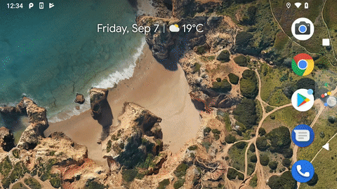
When hand motion is not present because the device is completely stabilized (e.g. placed on a tripod), we can still achieve our goal of simulating natural hand motion by intentionally “jiggling” the camera, by forcing the OIS module to move slightly between the shots. This movement is extremely small and chosen such that it doesn’t interfere with normal photos - but you can observe it yourself on Pixel 3 by holding the phone perfectly still, such as by pressing it against a window, and maximally pinch-zooming the viewfinder. Look for a tiny but continuous elliptical motion in distant objects, like that shown below.
Overcoming the Challenges of Super-resolution
The description of the ideal process we gave above sounds simple, but super-resolution is not that easy — there are many reasons why it hasn’t widely been used in consumer products like mobile phones, and requires the development of significant algorithmic innovations. Challenges can include:
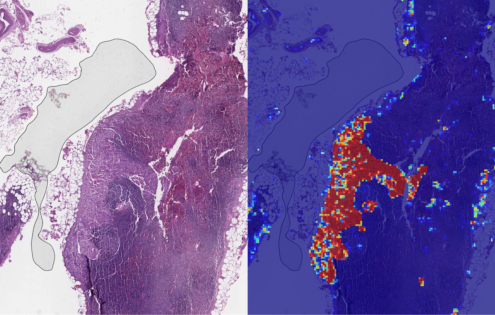
  • A single image from a burst is noisy, even in good lighting. A practical super-resolution algorithm needs to be aware of this noise and work correctly despite it. We don’t want to get just a higher resolution noisy image - our goal is to both increase the resolution but also produce a much less noisy result.
    Left: Single frame frame from a burst taken in good light conditions can still contain a substantial amount of noise due to underexposure. Right: Result of merging multiple frames after burst processing.
  • Motion between images in a burst is not limited to just the movement of the camera. There can be complex motions in the scene such as wind-blown leaves, ripples moving across the surface of water, cars, people moving or changing their facial expressions, or the flicker of a flame — even some movements that cannot be assigned a single, unique motion estimate because they are transparent or multi-layered, such as smoke or glass. Completely reliable and localized alignment is generally not possible, and therefore a good super-resolution algorithm needs to work even if motion estimation is imperfect.
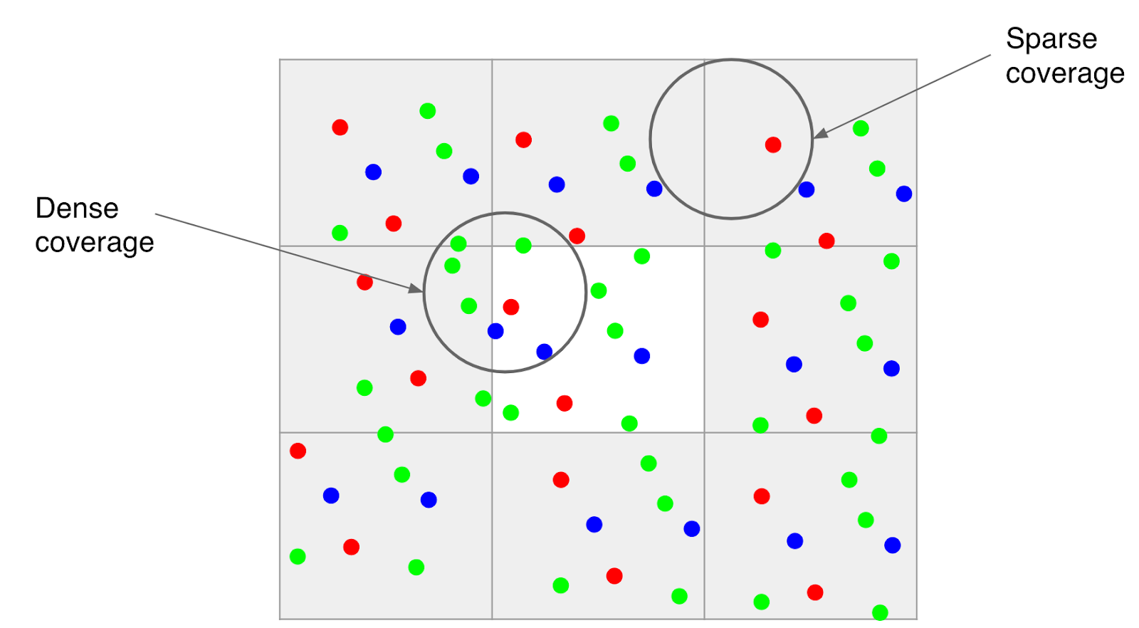
  • Because much of motion is random, even if there is good alignment, the data may be dense in some areas of the image and sparse in others. The crux of super-resolution is a complex interpolation problem, so the irregular spread of data makes it challenging to produce a higher-resolution image in all parts of the grid.
All the above challenges would seem to make real-world super-resolution either infeasible in practice, or at best limited to only static scenes and a camera placed on a tripod. With Super Res Zoom on Pixel 3, we’ve developed a stable and accurate burst resolution enhancement method that uses natural hand motion, and is robust and efficient enough to deploy on a mobile phone.

Here’s how we’ve addressed some of these challenges:
  • To effectively merge frames in a burst, and to produce a red, green, and blue value for every pixel without the need for demosaicing, we developed a method of integrating information across the frames that takes into account the edges of the image, and adapts accordingly. Specifically, we analyze the input frames and adjust how we combine them together, trading off increase in detail and resolution vs. noise suppression and smoothing. We accomplish this by merging pixels along the direction of apparent edges, rather than across them. The net effect is that our multi-frame method provides the best practical balance between noise reduction and enhancement of details.
    Left: Merged image with sub-optimal tradeoff of noise reduction and enhanced resolution. Right: The same merged image with a better tradeoff.
  • To make the algorithm handle scenes with complex local motion (people, cars, water or tree leaves moving) reliably, we developed a robustness model that detects and mitigates alignment errors. We select one frame as a “reference image”, and merge information from other frames into it only if we’re sure that we have found the correct corresponding feature. In this way, we can avoid artifacts like “ghosting” or motion blur, and wrongly merged parts of the image.
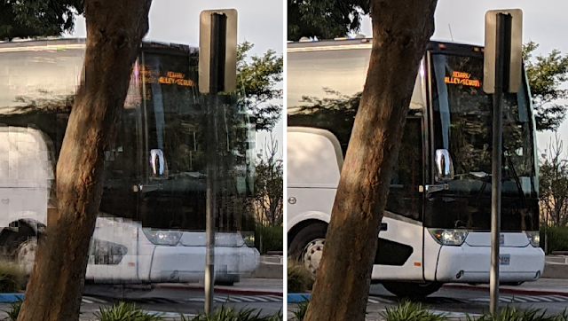
    A fast moving bus in a burst of images. Left: Merge without robustness model. Right: Merge with robustness model.
Pushing the State of the Art in Mobile Photography
The Portrait mode last year, and the HDR+ pipeline before it, showed how good mobile photography can be. This year, we set out to do the same for zoom. That’s another step in advancing the state of the art in computational photography, while shrinking the quality gap between mobile photography and DSLRs. Here is an album containing full FOV images, followed by Super Res Zoom images. Note that the Super Res Zoom images in this album are not cropped — they are captured directly on-device using pinch-zoom.
Left: Crop of 7x zoomed image on Pixel 2. Right: Same crop from Super Res Zoom on Pixel 3.
The idea of super-resolution predates the advent of smart-phones by at least a decade. For nearly as long, it has also lived in the public imagination through films and television. It’s been the subject of thousands of papers in academic journals and conferences. Now, it is real — in the palm of your hands, in Pixel 3.
An illustrative animation of Super Res Zoom. When the user takes a zoomed photo, the Pixel 3 takes advantage of the user’s natural hand motion and captures a burst of images at subtly different positions. These are then merged together to add detail to the final image.
Acknowledgements
Super Res Zoom is the result of a collaboration across several teams at Google. The project would not have been possible without the joint efforts of teams managed by Peyman Milanfar, Marc Levoy, and Bill Freeman. The authors would like to thank Marc Levoy and Isaac Reynolds in particular for their assistance in the writing of this blog.

The authors wish to especially acknowledge the following key contributors to the Super Res Zoom project: Ignacio Garcia-Dorado, Haomiao Jiang, Manfred Ernst, Michael Krainin, Daniel Vlasic, Jiawen Chen, Pascal Getreuer, and Chia-Kai Liang. The project also benefited greatly from contributions and feedback by Ce Liu, Damien Kelly, and Dillon Sharlet.


How to get the most out of Super Res Zoom?
Here are some tips on getting the best of Super Res Zoom on a Pixel 3 phone:
  • Pinch and zoom, or use the + button to increase zoom by discrete steps.
  • Double-tap the preview to quickly toggle between zoomed in and zoomed out.
  • Super Res works well at all zoom factors, though for performance reasons, it activates only above 1.2x. That’s about half way between no zoom and the first “click” in the zoom UI.
  • There are fundamental limits to the optical resolution of a wide-angle camera. So to get the most out of (any) zoom, keep the magnification factor modest.
  • Avoid fast moving objects. Super Res zoom will capture them correctly, but you will not likely get increased resolution.


* It’s worth noting that the situation is similar in some ways to how we see — in human (and other mammalian) eyes, different eye cone cells are sensitive to some specific colors, with the brain filling in the details to reconstruct the full image.

Source: Google AI Blog


Applying Deep Learning to Metastatic Breast Cancer Detection


A pathologist’s microscopic examination of a tumor in patients is considered the gold standard for cancer diagnosis, and has a profound impact on prognosis and treatment decisions. One important but laborious aspect of the pathologic review involves detecting cancer that has spread (metastasized) from the primary site to nearby lymph nodes. Detection of nodal metastasis is relevant for most cancers, and forms one of the foundations of the widely-used TNM cancer staging.

In breast cancer in particular, nodal metastasis influences treatment decisions regarding radiation therapy, chemotherapy, and the potential surgical removal of additional lymph nodes. As such, the accuracy and timeliness of identifying nodal metastases has a significant impact on clinical care. However, studies have shown that about 1 in 4 metastatic lymph node staging classifications would be changed upon second pathologic review, and detection sensitivity of small metastases on individual slides can be as low as 38% when reviewed under time constraints.

Last year, we described our deep learning–based approach to improve diagnostic accuracy (LYmph Node Assistant, or LYNA) to the 2016 ISBI Camelyon Challenge, which provided gigapixel-sized pathology slides of lymph nodes from breast cancer patients for researchers to develop computer algorithms to detect metastatic cancer. While LYNA achieved significantly higher cancer detection rates (Liu et al. 2017) than had been previously reported, an accurate algorithm alone is insufficient to improve pathologists’ workflow or improve outcomes for breast cancer patients. For patient safety, these algorithms must be tested in a variety of settings to understand their strengths and weaknesses. Furthermore, the actual benefits to pathologists using these algorithms had not been previously explored and must be assessed to determine whether or not an algorithm actually improves efficiency or diagnostic accuracy.

In “Artificial Intelligence Based Breast Cancer Nodal Metastasis Detection: Insights into the Black Box for Pathologists” (Liu et al. 2018), published in the Archives of Pathology and Laboratory Medicine and “Impact of Deep Learning Assistance on the Histopathologic Review of Lymph Nodes for Metastatic Breast Cancer” (Steiner, MacDonald, Liu et al. 2018) published in The American Journal of Surgical Pathology, we present a proof-of-concept pathologist assistance tool based on LYNA, and investigate these factors.

In the first paper, we applied our algorithm to de-identified pathology slides from both the Camelyon Challenge and an independent dataset provided by our co-authors at the Naval Medical Center San Diego. Because this additional dataset consisted of pathology samples from a different lab using different processes, it improved the representation of the diversity of slides and artifacts seen in routine clinical practice. LYNA proved robust to image variability and numerous histological artifacts, and achieved similar performance on both datasets without additional development.
Left: sample view of a slide containing lymph nodes, with multiple artifacts: the dark zone on the left is an air bubble, the white streaks are cutting artifacts, the red hue across some regions are hemorrhagic (containing blood), the tissue is necrotic (decaying), and the processing quality was poor. Right: LYNA identifies the tumor region in the center (red), and correctly classifies the surrounding artifact-laden regions as non-tumor (blue).
In both datasets, LYNA was able to correctly distinguish a slide with metastatic cancer from a slide without cancer 99% of the time. Further, LYNA was able to accurately pinpoint the location of both cancers and other suspicious regions within each slide, some of which were too small to be consistently detected by pathologists. As such, we reasoned that one potential benefit of LYNA could be to highlight these areas of concern for pathologists to review and determine the final diagnosis.

In our second paper, 6 board-certified pathologists completed a simulated diagnostic task in which they reviewed lymph nodes for metastatic breast cancer both with and without the assistance of LYNA. For the often laborious task of detecting small metastases (termed micrometastases), the use of LYNA made the task subjectively “easier” (according to pathologists’ self-reported diagnostic difficulty) and halved average slide review time, requiring about one minute instead of two minutes per slide.
Left: sample views of a slide containing lymph nodes with a small metastatic breast tumor at progressively higher magnifications. Right: the same views when shown with algorithmic “assistance” (LYmph Node Assistant, LYNA) outlining the tumor in cyan.
This suggests the intriguing potential for assistive technologies such as LYNA to reduce the burden of repetitive identification tasks and to allow more time and energy for pathologists to focus on other, more challenging clinical and diagnostic tasks. In terms of diagnostic accuracy, pathologists in this study were able to more reliably detect micrometastases with LYNA, reducing the rate of missed micrometastases by a factor of two. Encouragingly, pathologists with LYNA assistance were more accurate than either unassisted pathologists or the LYNA algorithm itself, suggesting that people and algorithms can work together effectively to perform better than either alone.

With these studies, we have made progress in demonstrating the robustness of our LYNA algorithm to support one component of breast cancer TNM staging, and assessing its impact in a proof-of-concept diagnostic setting. While encouraging, the bench-to-bedside journey to help doctors and patients with these types of technologies is a long one. These studies have important limitations, such as limited dataset sizes and a simulated diagnostic workflow which examined only a single lymph node slide for every patient instead of the multiple slides that are common for a complete clinical case. Further work will be needed to assess the impact of LYNA on real clinical workflows and patient outcomes. However, we remain optimistic that carefully validated deep learning technologies and well-designed clinical tools can help improve both the accuracy and availability of pathologic diagnosis around the world.

Source: Google AI Blog


Open Sourcing Active Question Reformulation with Reinforcement Learning


Natural language understanding is a significant ongoing focus of Google’s AI research, with application to machine translation, syntactic and semantic parsing, and much more. Importantly, as conversational technology increasingly requires the ability to directly answer users’ questions, one of the most active areas of research we pursue is question answering (QA), a fundamental building block of human dialogue.

Because open sourcing code is a critical component of reproducible research, we are releasing a TensorFlow package for Active Question Answering (ActiveQA), a research project that investigates using reinforcement learning to train artificial agents for question answering. Introduced for the first time in our ICLR 2018 paper “Ask the Right Questions: Active Question Reformulation with Reinforcement Learning”, ActiveQA interacts with QA systems using natural language with the goal of providing better answers.

Active Question Answering
In traditional QA, supervised learning techniques are used in combination with labeled data to train a system that answers arbitrary input questions. While this is effective, it suffers from a lack of ability to deal with uncertainty like humans would, by reformulating questions, issuing multiple searches, evaluating and aggregating responses. Inspired by humans’ ability to "ask the right questions", ActiveQA introduces an agent that repeatedly consults the QA system. In doing so, the agent may reformulate the original question multiple times in order to find the best possible answer. We call this approach active because the agent engages in a dynamic interaction with the QA system, with the goal of improving the quality of the answers returned.

For example, consider the question “When was Tesla born?”. The agent reformulates the question in two different ways: “When is Tesla’s birthday” and “Which year was Tesla born”, retrieving answers to both questions from the QA system. Using all this information it decides to return “July 10 1856”.
What characterizes an ActiveQA system is that it learns to ask questions that lead to good answers. However, because training data in the form of question pairs, with an original question and a more successful variant, is not readily available, ActiveQA uses reinforcement learning, an approach to machine learning concerned with training agents so that they take actions that maximize a reward, while interacting with an environment.

The learning takes place as the ActiveQA agent interacts with the QA system; each question reformulation is evaluated in terms of how good the corresponding answer is, which constitutes the reward. If the answer is good, then the learning algorithm will adjust the model’s parameters so that the question reformulation that lead to the answer is more likely to be generated again, or otherwise less likely, if the answer was bad.

In our paper, we show that it is possible to train such agents to outperform the underlying QA system, the one used to provide answers to reformulations, by asking better questions. This is an important result, as the QA system is already trained with supervised learning to solve the same task. Another compelling finding of our research is that the ActiveQA agent can learn a fairly sophisticated, and still somewhat interpretable, reformulation strategy (the policy in reinforcement learning). The learned policy uses well-known information retrieval techniques such as tf-idf query term re-weighting, the process by which more informative terms are weighted more than generic ones, and word stemming.

Build Your Own ActiveQA System
The TensorFlow ActiveQA package we are releasing consists of three main components, and contains all the code necessary to train and run the ActiveQA agent.
  • A pretrained sequence to sequence model that takes as input a question and returns its reformulations. This task is similar to machine translation, translating from English to English, and indeed the initial model can be used for general paraphrasing. For its implementation we use and customize the TensorFlow Neural Machine Translation Tutorial code. We adapted the code to support training with reinforcement learning, using policy gradient methods.*
  • An answer selection model. The answer selector uses a convolutional neural network and assigns a score to each triplet of original question, reformulation and answer. The selector uses pre-trained, publicly available word embeddings (GloVe).
  • A question answering system (the environment). For this purpose we use BiDAF, a popular question answering system, described in Seo et al. (2017).
We also provide pointers to checkpoints for all the trained models.

Google’s mission is to organize the world's information and make it universally accessible and useful, and we believe that ActiveQA is an important step in realizing that mission. We envision that this research will help us design systems that provide better and more interpretable answers, and hope it will help others develop systems that can interact with the world using natural language.

Acknowledgments
Contributors to this research and release include Alham Fikri Aji, Christian Buck, Jannis Bulian, Massimiliano Ciaramita, Wojciech Gajewski, Andrea Gesmundo, Alexey Gronskiy, Neil Houlsby, Yannic Kilcher, and Wei Wang.


* The system we reported on in our paper used the TensorFlow sequence-to-sequence code used in Britz et al. (2017). Later, an open source version of the Google Translation model (GNMT) was published as a tutorial. The ActiveQA version released today is based on this more recent, and actively developed implementation. For this reason the released system varies slightly from the paper’s. Nevertheless, the performance and behavior are qualitatively and quantitatively comparable.

Source: Google AI Blog


Highlights from the Google AI Residency Program


In 2016, we welcomed the inaugural class of the Google Brain Residency, a select group of 27 individuals participating in a 12-month program focused on jump-starting a career in machine learning and deep learning research. Since then, the program has experienced rapid growth, leading to its evolution into the Google AI Residency, which serves to provide residents the opportunity to embed themselves within the broader group of Google AI teams working on machine learning research and its applications.
Some of our 2017 Google AI residents at the 2017 Neural Information Processing Systems Conference, hosted in Long Beach, California.
The accomplishments of the second class of residents are as remarkable as those of the first, publishing multiple works to various top-tier machine learning, robotics and healthcare conferences and journals. Publication topics include:
  • A study on the effect of adversarial examples on human visual perception.
  • An algorithm that enables robots to learn more safely by avoiding states from which they cannot reset.
  • Initialization methods which enable training of neural network with unprecedented depths of 10K+ layers.
  • A method to make training more scalable by using larger mini-batches, which when applied to ResNet-50 on ImageNet reduced training time without compromising test accuracy.
  • And many more...
This experiment demonstrated (for the first time) the susceptibility of human time-limited vision to adversarial examples. For more details, see “Adversarial Examples that Fool both Computer Vision and Time-Limited Humans” accepted at NIPS 2018).
An algorithm for safe reinforcement learning prevents robots from taking actions they cannot undo. For more details, see “Leave no Trace: Learning to Reset for Safe and Autonomous Reinforcement Learning” (accepted at ICLR 2018).
Extremely deep CNNs can be trained without the use of any special tricks simply by using a specially designed (Delta-Orthogonal) initialization. Test (solid) and training (dashed) curves on MNIST (top) and CIFAR10 (bottom). For more details, see “Dynamical Isometry and a Mean Field Theory of CNNs: How to Train 10,000-Layer Vanilla Convolutional Neural Networks” accepted at ICML 2018.
Applying a sequence of simple scaling rules, we increase the SGD batch size and reduce the number of parameter updates required to train our model by an order of magnitude, without sacrificing test set accuracy. This enables us to dramatically reduce model training time. For more details, see “Don’t Decay the Learning Rate, Increase the Batch Size”, accepted at ICLR 2018.
With the 2017 class of Google AI residents graduated and off to pursue the next exciting phase in their careers, their desks were quickly filled in June by the 2018 class. Furthermore, this new class is the first to be embedded in various teams across Google’s global offices, pursuing research in areas such as perception, algorithms and optimization, language, healthcare and much more. We look forward to seeing what they can accomplish and contribute to the broader research community!

If you are interested in joining the fourth class, applications for the 2019 Google AI Residency program are now open! Visit g.co/airesidency/apply for more information on how to apply. Also, check out g.co/airesidency to see more resident profiles, past Resident publications, blog posts and stories. We can’t wait to see where the next year will take us, and hope you’ll collaborate with our research teams across the world!

Source: Google AI Blog


Introducing the Kaggle “Quick, Draw!” Doodle Recognition Challenge


Online handwriting recognition consists of recognizing structured patterns in freeform handwritten input. While Google products like Translate, Keep and Handwriting Input use this technology to recognize handwritten text, it works for any predefined pattern for which enough training data is available. The same technology that lets you digitize handwritten text can also be used to improve your drawing abilities and build virtual worlds, and represents an exciting research direction that explores the potential of handwriting as a human-computer interaction modality. For example the “Quick, Draw!” game generated a dataset of 50M drawings (out of more than 1B that were drawn) which itself inspired many different new projects.

In order to encourage further research in this exciting field, we have launched the Kaggle "Quick, Draw!" Doodle Recognition Challenge, which tasks participants to build a better machine learning classifier for the existing “Quick, Draw!” dataset. Importantly, since the training data comes from the game itself (where drawings can be incomplete or may not match the label), this challenge requires the development of a classifier that can effectively learn from noisy data and perform well on a manually-labeled test set from a different distribution.

The Dataset
In the original “Quick, Draw!” game, the player is prompted to draw an image of a certain category (dog, cow, car, etc). The player then has 20 seconds to complete the drawing - if the computer recognizes the drawing correctly within that time, the player earns a point. Each game consists of 6 randomly chosen categories.
Because of the game mechanics, the labels in the Quick, Draw! dataset fall into the following categories:
  • Correct: the user drew the prompted category and the computer only recognized it correctly after the user was done drawing.
  • Correct, but incomplete: the user drew the prompted category and the computer recognized it correctly before the user had finished. Incompleteness can vary from nearly ready to only a fraction of the category drawn. This is probably fairly common in images that are marked as recognized correctly.
  • Correct, but not recognized correctly: The player drew the correct category but the AI never recognized it. Some players react to this by adding more details. Others scribble out and try again.
  • Incorrect: some players have different concepts in mind when they see a word - e.g. in the category seesaw, we have observed a number of saw drawings.
In addition to the labels described above, each drawing is given as a sequence of strokes, where each stroke is a sequence of touch points. While these can easily be rendered as images, using the order and direction of strokes often helps making handwriting recognizers better.

Get Started
We’ve previously published a tutorial that uses this dataset, and now we're inviting the community to build on this or other approaches to achieve even higher accuracy. You can get started by visiting the challenge website and going through the existing kernels which allow you to analyze the data and visualize it. We’re looking forward to learning about the approaches that the community comes up with for the competition and how much you can improve on our original production model.

Acknowledgements
We'd like to thank everyone who worked with us on this, particularly Jonas Jongejan and Brenda Fogg from the Creative Lab team, Julia Elliott and Walter Reade from the Kaggle team, and the handwriting recognition team.

Source: Google AI Blog


Building Google Dataset Search and Fostering an Open Data Ecosystem


Earlier this month we launched Google Dataset Search, a tool designed to make it easier for researchers to discover datasets that can help with their work. What we colloquially call "Google Scholar for data,” Google Dataset Search is a search engine across metadata for millions of datasets in thousands of repositories across the Web. In this post, we go into some detail of how Dataset Search is built, outlining what we believe will help develop an open data ecosystem, and we also address the question that we received frequently since the Dataset Search launch, "Why is my dataset not showing up in Google Dataset Search?

An Overview
At a very high level, Google Data Search relies on dataset providers, big and small, adding structured metadata on their sites using the open schema.org/Dataset standard. The metadata specifies the salient properties of each dataset: its name and description, spatial and temporal coverage, provenance information, and so on. Dataset Search uses this metadata, links it with other resources that are available at Google (more on this below!), and builds an index of this enriched corpus of metadata. Once we built the index, we can start answering user queries — and figuring out which results best correspond to the query.
An overview of the technology behind Google Dataset Search
Using Structured Metadata from Data Providers
When Google's search engine processes a Web page with schema.org/Dataset mark-up, it understands that there is dataset metadata there and processes that structured metadata to create "records" describing each annotated dataset on a page. The use of schema.org allows developers to embed this structured information into HTML, without affecting the appearance of the page while making the semantics of the information visible to all search engines.

However, no matter how precise schema.org definitions or guidelines are, some metadata will inevitably be incomplete, wrong, or entirely missing. Furthermore, distinctions between some fields can be vague: is the dataset repository a publisher or a provider of a dataset? How do we distinguish between citations to a scientific paper that describes the creation of the dataset vs. papers describing its use? Indeed, many of these questions often generate active scholarly discussions.

Despite these variations, Dataset Search must provide a uniform and predictable user experience on the front end. Therefore, in some cases we substitute a more general field name (e.g., “provided by”) to display the values coming from multiple other fields (e.g., “publisher”, “creator”, etc.). In other cases, we are not able to use some of the fields at all: if a specific field is being misinterpreted in many different ways by dataset providers, we bypass that field for now and work with the community to clarify the guidelines. In each decision, we had one specific question that helped us in difficult cases "What will help data discovery the most?" This focus on the task that we were addressing made some of the problems easier than they seemed at first.

Connecting Replicas of Datasets
It is very common for a dataset, in particular a popular one, to be present in more than one repository. We use a variety of signals to determine when two datasets are replicas of each other. For example, schema.org has a way to specify the connection explicitly, through schema.org/sameAs, which is the best way to link different replicas together and to point to the canonical source of a dataset. Other signals include two datasets descriptions pointing to the same canonical page, having the same Digital Object Identifier (DOI), sharing links for downloading the dataset, or having a large overlap in other metadata fields. None of these signals are perfect in isolation, therefore we combine them to get the strongest possible indication of when two datasets are the same.

Reconciling to the Google Knowledge Graph
Google's Knowledge Graph is a powerful platform that describes and links information about many entities, including the ones that appear in dataset metadata: organizations providing datasets, locations for spatial coverage of the data, funding agencies, and so on. Therefore, we try to reconcile information mentioned in the metadata fields with the items in the Knowledge Graph. We can do this reconciliation with good precision for two main reasons. First, we know the types of items in the Knowledge Graph and the types of entities that we expect in the metadata fields. Therefore, we can limit the types of entities from the Knowledge Graph that we match with values for a particular metadata field. For example, a provider of a dataset should match with an organization entity in the Knowledge Graph and not with, say, a location. Second, the context of the Web page itself helps reduce the number of choices, which is particularly useful for distinguishing between organizations that share the same acronym. For example, the acronym CAMRA can stand for “Chilbolton Advanced Meteorological Radar” or “Campaign for Real Ale”. If we use terms from the Web page, we can then more easily determine that CAMRA is in fact the Chilbolton Radar when we see terms such as “clouds”, “vapor”, and “water” on the page.

This type of reconciliation opens up lots of possibilities to improve the search experience for users. For instance, Dataset Search can localize results by showing reconciled values of metadata in the same language as the rest of the page. Additionally, it can rely on synonyms, correct misspellings, expand acronyms, or use other relations in the Knowledge Graph for query expansion.

Linking to other Google Resources
Google has many other data resources that are useful in augmenting the dataset metadata, such as Google Scholar. Knowing which datasets are referenced and cited in publications serves at least two purposes:
  1. It provides a valuable signal about the importance and prominence of a dataset.
  2. It gives dataset authors an easy place to see citations to their data and to get credit.
Indeed, we hope that highlighting publications that use the data will lead to a more healthy ecosystem of data citation. For the moment, our links to Google scholar are very approximate as we lack a good model on how people cite data. We try to go beyond DOIs to give somewhat better coverage, but the number of articles citing a dataset ends up being approximate. We hope to make more progress in this area in order to get a higher level of precision.

Search and Ranking of Results
When a user issues a query, we search through the corpus of datasets, in a way not unlike Google Search works over Web pages. Just like with any search, we need to determine whether a document is relevant for the query and then rank the relevant documents. Because there are no large-scale studies on how users search for datasets, as a first approximation, we rely on Google Web ranking. However, ranking datasets is different from ranking Web pages, and we add some additional signals that take into account the metadata quality, citations, and so on. As Dataset Search gets used more by our users and we understand better how users search for datasets, we hope that ranking will improve significantly.

A Better Open Data Ecosystem
We built Dataset Search in an attempt to create a tool that will positively impact the discoverability of data. The decision to rely on open standards (schema.org, W3C DCAT, JSON-LD, etc.) for markup is intentional, as Dataset Search can only be as good as the open-data ecosystem that it supports. As such, Google Dataset Search aims to support a strong open data ecosystem by encouraging:
  1. Widespread adoption of open metadata formats to describe published data.
  2. Further development of open metadata formats to describe more types of data and in more detail.
  3. The culture of citing data the way we cite research publications, giving those who create and publish the data the credit that they deserve.
  4. The development of tools that leverage this metadata to enable more discovery or better use of data. 
The increased adoption of open metadata standards in conjunction with the continued development of Dataset Search (and, hopefully, other tools) should foster a healthier open data ecosystem where data is a first-class citizen of research.

So, Where is Your Dataset?
It is probably clear by now that Dataset Search is only as good as the metadata that exists on the Web pages for datasets. The most common answer to the question of why a specific dataset does not show up in our results is that the Web page for that dataset does not have any markup. Just pop that page into the Structured Data Testing Tool and you will see whether the markup is there. If you don't see any markup there, and you own the page, you can add it and if you don't own the page, you can ask the page owners to do it, which will make their page more easily discoverable by everyone.

We hope that the community finds Dataset Search useful, users make serendipitous discoveries and save time and scientists and journalists spend less time searching for data and more time using it.

Acknowledgements
We would like to thank Xiaomeng Ban, Dan Brickley, Lee Butler, Thomas Chen, Corinna Cortes, Kevin Espinoza, Archana Jain, Mike Jones, Kishore Papineni, Chris Sater, Gokhan Turhan, Shubin Zhao and Andi Vajda for their work on the project and all our partners, collaborators, and early adopters for their help.

Source: Google AI Blog


Google’s Next Generation Music Recognition


In 2017 we launched Now Playing on the Pixel 2, using deep neural networks to bring low-power, always-on music recognition to mobile devices. In developing Now Playing, our goal was to create a small, efficient music recognizer which requires a very small fingerprint for each track in the database, allowing music recognition to be run entirely on-device without an internet connection. As it turns out, Now Playing was not only useful for an on-device music recognizer, but also greatly exceeded the accuracy and efficiency of our then-current server-side system, Sound Search, which was built before the widespread use of deep neural networks. Naturally, we wondered if we could bring the same technology that powers Now Playing to the server-side Sound Search, with the goal of making Google’s music recognition capabilities the best in the world.

Recently, we introduced a new version of Sound Search that is powered by some of the same technology used by Now Playing. You can use it through the Google Search app or the Google Assistant on any Android phone. Just start a voice query, and if there’s music playing near you, a “What’s this song?” suggestion will pop up for you to press. Otherwise, you can just ask, “Hey Google, what’s this song?” With this latest version of Sound Search, you’ll get faster, more accurate results than ever before!
Now Playing versus Sound Search
Now Playing miniaturized music recognition technology such that it was small and efficient enough to be run continuously on a mobile device without noticeable battery impact. To do this we developed an entirely new system using convolutional neural networks to turn a few seconds of audio into a unique “fingerprint.” This fingerprint is then compared against an on-device database holding tens of thousands of songs, which is regularly updated to add newly released tracks and remove those that are no longer popular. In contrast, the server-side Sound Search system is very different, having to match against ~1000x as many songs as Now Playing. Making Sound Search both faster and more accurate with a substantially larger musical library presented several unique challenges. But before we go into that, a few details on how Now Playing works.

The Core Matching Process of Now Playing
Now Playing generates the musical “fingerprint” by projecting the musical features of an eight-second portion of audio into a sequence of low-dimensional embedding spaces consisting of seven two-second clips at 1 second intervals, giving a segmentation like this:
Now Playing then searches the on-device song database, which was generated by processing popular music with the same neural network, for similar embedding sequences. The database search uses a two phase algorithm to identify matching songs, where the first phase uses a fast but inaccurate algorithm which searches the whole song database to find a few likely candidates, and the second phase does a detailed analysis of each candidate to work out which song, if any, is the right one.
  • Matching, phase 1: Finding good candidates: For every embedding, Now Playing performs a nearest neighbor search on the on-device database of songs for similar embeddings. The database uses a hybrid of spatial partitioning and vector quantization to efficiently search through millions of embedding vectors. Because the audio buffer is noisy, this search is approximate, and not every embedding will find a nearby match in the database for the correct song. However, over the whole clip, the chances of finding several nearby embeddings for the correct song are very high, so the search is narrowed to a small set of songs which got multiple hits.
  • Matching, phase 2: Final matching: Because the database search used above is approximate, Now Playing may not find song embeddings which are nearby to some embeddings in our query. Therefore, in order to calculate an accurate similarity score, Now Playing retrieves all embeddings for each song in the database which might be relevant to fill in the “gaps”. Then, given the sequence of embeddings from the audio buffer and another sequence of embeddings from a song in the on-device database, Now Playing estimates their similarity pairwise and adds up the estimates to get the final matching score.
It’s critical to the accuracy of Now Playing to use a sequence of embeddings rather than a single embedding. The fingerprinting neural network is not accurate enough to allow identification of a song from a single embedding alone — each embedding will generate a lot of false positive results. However, combining the results from multiple embeddings allows the false positives to be easily removed, as the correct song will be a match to every embedding, while false positive matches will only be close to one or two embeddings from the input audio.

Scaling up Now Playing for the Sound Search server
So far, we’ve gone into some detail of how Now Playing matches songs to an on-device database. The biggest challenge in going from Now Playing, with tens of thousands of songs, to Sound Search, with tens of millions, is that there are a thousand times as many songs which could give a false positive result. To compensate for this without any other changes, we would have to increase the recognition threshold, which would mean needing more audio to get a confirmed match. However, the goal of the new Sound Search server was to be able to match faster, not slower, than Now Playing, so we didn’t want people to wait 10+ seconds for a result.

As Sound Search is a server-side system, it isn’t limited by processing and storage constraints in the same way Now Playing is. Therefore, we made two major changes to how we do fingerprinting, both of which increased accuracy at the expense of server resources:
  • We quadrupled the size of the neural network used, and increased each embedding from 96 to 128 dimensions, which reduces the amount of work the neural network has to do to pack the high-dimensional input audio into a low-dimensional embedding. This is critical in improving the quality of phase two, which is very dependent on the accuracy of the raw neural network output.
  • We doubled the density of our embeddings — it turns out that fingerprinting audio every 0.5s instead of every 1s doesn’t reduce the quality of the individual embeddings very much, and gives us a huge boost by doubling the number of embeddings we can use for the match.
We also decided to weight our index based on song popularity - in effect, for popular songs, we lower the matching threshold, and we raise it for obscure songs. Overall, this means that we can keep adding more (obscure) songs almost indefinitely to our database without slowing our recognition speed too much.

Conclusion
With Now Playing, we originally set out to use machine learning to create a robust audio fingerprint compact enough to run entirely on a phone. It turned out that we had, in fact, created a very good all-round audio fingerprinting system, and the ideas developed there carried over very well to the server-side Sound Search system, even though the challenges of Sound Search are quite different.

We still think there’s room for improvement though — we don’t always match when music is very quiet or in very noisy environments, and we believe we can make the system even faster. We are continuing to work on these challenges with the goal of providing the next generation in music recognition. We hope you’ll try it the next time you want to find out what song is playing! You can put a shortcut on your home screen like this:
Acknowledgements
We would like to thank Micha Riser, Mihajlo Velimirovic, Marvin Ritter, Ruiqi Guo, Sanjiv Kumar, Stephen Wu, Diego Melendo Casado‎, Katia Naliuka, Jason Sanders, Beat Gfeller, Christian Frank, Dominik Roblek, Matt Sharifi and Blaise Aguera y Arcas‎.

Source: Google AI Blog


Introducing the Unrestricted Adversarial Examples Challenge


Machine learning is being deployed in more and more real-world applications, including medicine, chemistry and agriculture. When it comes to deploying machine learning in safety-critical contexts, significant challenges remain. In particular, all known machine learning algorithms are vulnerable to adversarial examples — inputs that an attacker has intentionally designed to cause the model to make a mistake. While previous research on adversarial examples has mostly focused on investigating mistakes caused by small modifications in order to develop improved models, real-world adversarial agents are often not subject to the “small modification” constraint. Furthermore, machine learning algorithms can often make confident errors when faced with an adversary, which makes the development of classifiers that don’t make any confident mistakes, even in the presence of an adversary which can submit arbitrary inputs to try to fool the system, an important open problem.

Today we're announcing the Unrestricted Adversarial Examples Challenge, a community-based challenge to incentivize and measure progress towards the goal of zero confident classification errors in machine learning models. While previous research has focused on adversarial examples that are restricted to small changes to pre-labeled data points (allowing researchers to assume the image should have the same label after a small perturbation), this challenge allows unrestricted inputs, allowing participants to submit arbitrary images from the target classes to develop and test models on a wider variety of adversarial examples.
Adversarial examples can be generated through a variety of means, including by making small modifications to the input pixels, but also using spatial transformations, or simple guess-and-check to find misclassified inputs.
Structure of the Challenge
Participants can submit entries one of two roles: as a defender, by submitting a classifier which has been designed to be difficult to fool, or as an attacker, by submitting arbitrary inputs to try to fool the defenders' models. In a “warm-up” period before the challenge, we will present a set of fixed attacks for participants to design networks to defend against. After the community can conclusively beat those fixed attacks, we will launch the full two-sided challenge with prizes for both attacks and defenses.

For the purposes of this challenge, we have created a simple “bird-or-bicycle” classification task, where a classifier must answer the following: “Is this an unambiguous picture of a bird, a bicycle, or is it ambiguous / not obvious?” We selected this task because telling birds and bicycles apart is very easy for humans, but all known machine learning techniques struggle at the task when in the presence of an adversary.

The defender's goal is to correctly label a clean test set of birds and bicycles with high accuracy, while also making no confident errors on any attacker-provided bird or bicycle image. The attacker's goal is to find an image of a bird that the defending classifier confidently labels as a bicycle (or vice versa). We want to make the challenge as easy as possible for the defenders, so we discard all images that are ambiguous (such as a bird riding a bicycle) or not obvious (such as an aerial view of a park, or random noise).
Examples of ambiguous and unambiguous images. Defenders must make no confident mistakes on unambiguous bird or bicycle images. We discard all images that humans find ambiguous or not obvious. All images under CC licenses 1, 2, 3, 4.
Attackers may submit absolutely any image of a bird or a bicycle in an attempt to fool the defending classifier. For example, an attacker could take photographs of birds, use 3D rendering software, make image composites using image editing software, produce novel bird images with a generative model, or any other technique.

In order to validate new attacker-provided images, we ask an ensemble of humans to label the image. This procedure lets us allow attackers to submit arbitrary images, not just test set images modified in small ways. If the defending classifier confidently classifies as "bird" any attacker-provided image which the human labelers unanimously labeled as a bicycle, the defending model has been broken. You can learn more details about the structure of the challenge in our paper.

How to Participate
If you’re interested in participating, guidelines for getting started can be found on the project on github. We’ve already released our dataset, the evaluation pipeline, and baseline attacks for the warm-up, and we’ll be keeping an up-to-date leaderboard with the best defenses from the community. We look forward to your entries!

Acknowledgements
The team behind the Unrestricted Adversarial Examples Challenge includes Tom Brown, Catherine Olsson, Nicholas Carlini, Chiyuan Zhang, and Ian Goodfellow from Google, and Paul Christiano from OpenAI.

Source: Google AI Blog


The What-If Tool: Code-Free Probing of Machine Learning Models


Building effective machine learning (ML) systems means asking a lot of questions. It's not enough to train a model and walk away. Instead, good practitioners act as detectives, probing to understand their model better: How would changes to a datapoint affect my model’s prediction? Does it perform differently for various groups–for example, historically marginalized people? How diverse is the dataset I am testing my model on?

Answering these kinds of questions isn’t easy. Probing “what if” scenarios often means writing custom, one-off code to analyze a specific model. Not only is this process inefficient, it makes it hard for non-programmers to participate in the process of shaping and improving ML models. One focus of the Google AI PAIR initiative is making it easier for a broad set of people to examine, evaluate, and debug ML systems.

Today, we are launching the What-If Tool, a new feature of the open-source TensorBoard web application, which let users analyze an ML model without writing code. Given pointers to a TensorFlow model and a dataset, the What-If Tool offers an interactive visual interface for exploring model results.
The What-If Tool, showing a set of 250 face pictures and their results from a model that detects smiles.
The What-If Tool has a large set of features, including visualizing your dataset automatically using Facets, the ability to manually edit examples from your dataset and see the effect of those changes, and automatic generation of partial dependence plots which show how the model’s predictions change as any single feature is changed. Let’s explore two features in more detail.
Exploring what-if scenarios on a datapoint.
Counterfactuals
With a click of a button you can compare a datapoint to the most similar point where your model predicts a different result. We call such points "counterfactuals," and they can shed light on the decision boundaries of your model. Or, you can edit a datapoint by hand and explore how the model’s prediction changes. In the screenshot below, the tool is being used on a binary classification model that predicts whether a person earns more than $50k based on public census data from the UCI census dataset. This is a benchmark prediction task used by ML researchers, especially when analyzing algorithmic fairness — a topic we'll get to soon. In this case, for the selected datapoint, the model predicted with 73% confidence that the person earns more than $50k. The tool has automatically located the most-similar person in the dataset for which the model predicted earnings of less than $50k and compares the two side-by-side. In this case, with just a minor difference in age and an occupation change, the model’s prediction has flipped.
Comparing counterfactuals.
Analysis of Performance and Algorithmic Fairness
You can also explore the effects of different classification thresholds, taking into account constraints such as different numerical fairness criteria. The below screenshot shows the results of a smile detector model, trained on the open-source CelebA dataset which consists of annotated face images of celebrities. Below, the faces in the dataset are divided by whether they have brown hair, and for each of the two groups there is an ROC curve and confusion matrix of the predictions, along with sliders for setting how confident the model must be before determining that a face is smiling. In this case, the confidence thresholds for the two groups were set automatically by the tool to optimize for equal opportunity.
Comparing the performance of two slices of data on a smile detection model, with their classification thresholds set to satisfy the “equal opportunity” constraint.
Demos
To illustrate the capabilities of the What-If Tool, we’ve released a set of demos using pre-trained models:
  • Detecting misclassifications: A multiclass classification model, which predicts plant type from four measurements of a flower from the plant. The tool is helpful in showing the decision boundary of the model and what causes misclassifications. This model is trained with the UCI iris dataset.
  • Assessing fairness in binary classification models: The image classification model for smile detection mentioned above. The tool is helpful in assessing algorithmic fairness across different subgroups. The model was purposefully trained without providing any examples from a specific subset of the population, in order to show how the tool can help uncover such biases in models. Assessing fairness requires careful consideration of the overall context — but this is a useful quantitative starting point.
  • Investigating model performance across different subgroups: A regression model that predicts a subject’s age from census information. The tool is helpful in showing relative performance of the model across subgroups and how the different features individually affect the prediction. This model is trained with the UCI census dataset.
What-If in Practice
We tested the What-If Tool with teams inside Google and saw the immediate value of such a tool. One team quickly found that their model was incorrectly ignoring an entire feature of their dataset, leading them to fix a previously-undiscovered code bug. Another team used it to visually organize their examples from best to worst performance, leading them to discover patterns about the types of examples their model was underperforming on.

We look forward to people inside and outside of Google using this tool to better understand ML models and to begin assessing fairness. And as the code is open-source, we welcome contributions to the tool.

Acknowledgments
The What-If Tool was a collaborative effort, with UX design by Mahima Pushkarna, Facets updates by Jimbo Wilson, and input from many others. We would like to thank the Google teams that piloted the tool and provided valuable feedback and the TensorBoard team for all their help.

Source: Google AI Blog


Text-to-Speech for Low-Resource Languages (Episode 4): One Down, 299 to Go


This is the fourth episode in the series of posts reporting on the work we are doing to build text-to-speech (TTS) systems for low resource languages. In the first episode, we described the crowdsourced acoustic data collection effort for Project Unison. In the second episode, we described how we built parametric voices based on that data. In the third episode, we described the compilation of a pronunciation lexicon for a TTS system. In this episode, we describe how to make a single TTS system speak many languages.

Developing TTS systems for any given language is a significant challenge, and requires large amounts of high quality acoustic recordings and linguistic annotations. Because of this, these systems are only available for a tiny fraction of the world's languages. A natural question that arises in this situation is, instead of attempting to build a high quality voice for a single language using monolingual data from multiple speakers, as we described in the previous three episodes, can we somehow combine the limited monolingual data from multiple speakers of multiple languages to build a single multilingual voice that can speak any language?

Building upon an initial investigation into creating a multilingual TTS system that can synthesize speech in multiple languages from a single model, we developed a new model that uses uniform phonological representation for all languages — the International Phonetic Alphabet (IPA). The model trained using this representation can synthesize both the languages seen in the training data as well as languages not observed in training. This has two main benefits: First, pooling training data from related languages increases phonemic coverage which results in improved synthesis quality of the languages observed in training. Finally, because the model contains many languages pooled together, there is a better chance that an “unseen” language will have a “related” language present in the model that will guide and aid the synthesis.

Exploring the Closely Related Languages of Indonesia
We applied this multilingual approach first to languages of Indonesia, where Standard Indonesian is the official national language, and is spoken natively or as a second language by more than 200 million people. Javanese, with roughly 90 million native speakers, and Sundanese, with approximately 40 million native speakers, constitute the two largest regional languages of Indonesia. Unlike Indonesian, which received a lot of attention by the computational linguists and speech scientists over the years, both Javanese and Sundanese are currently low-resourced due to the lack of openly available high-quality corpora. We collaborated with universities in Indonesia to collect crowd-sourced Javanese and Sundanese recordings.

Since our corpus of Standard Indonesian was much larger and recorded in a professional studio, our hypothesis was that combining three languages may result in significant improvements over the systems constructed using a “classical” monolingual approach. To test this, we first proceeded to analyze the similarities and crucial differences between the phonologies of these three languages (shown below) and used this information to design the phonological representation that allows maximum degree of sharing between the languages while preserving their crucial differences.
Joint phoneme inventory of Indonesian, Javanese, and Sundanese in International Phonetic Alphabet notation.
The resulting Javanese and Sundanese voices trained jointly with Standard Indonesian strongly outperformed our corresponding monolingual multispeaker voices that we used as a baseline. This allowed us to launch Javanese and Sundanese TTS in Google products, such as Google Translate and Android.

Expanding to the More Diverse Language Families of South Asia
Next, we focused on the languages of South Asia spanning two very different language families: Indo-Aryan and Dravidian. Unlike the languages of Indonesia described above, these languages are much more diverse. In particular, they have significantly smaller overlap in their phonologies. The table below shows a superset of the languages in our experiment, including the variety of orthographies used, as well as modern words related to the Sanskrit word for “culture”. These languages show considerable variation within each group, but also such similarities across groups.
Descendants of Sanskrit word for “culture” across languages.
In this work, we leveraged the unified phonological representation mentioned above to make the most of the data we have and eliminate scarcity of data for certain phonemes. This was accomplished by conflating similar phonemes into a single representative phoneme in the multilingual phoneme inventory. Where possible, we use the same inventory for phonologically close languages. For example we have an identical phoneme inventory for Telugu and Kannada, and another one for West Bengali and Odia. For other language pairs like Gujarati and Marathi, we copied over the inventory of one language to another, but made a few changes to reflect the differences in their phonemic inventories. For all languages in these experiments we retained a common underlying representation, mapping similar phonemes across different inventories, so that we could still use the data from one language in training the others.

In addition, we made sure our representation is driven by the phonology in use, rather than the orthography. For example, although there are distinct letters for long and short vowels in Marathi, they are not contrastive in a linguistic sense, so we used a single representation for them, increasing the robustness of our training data. Similarly, if two languages use one character that was historically related to the same Sanskrit letter to represent different sounds or different letters for a similar sound, our mapping reflected the phonological closeness rather than the historical or orthographic representation. Describing all the features of the unified phoneme inventory is outside the scope of this post, the details can be found in our recent paper.
Diagram illustrating our multilingual text-to-speech approach. The input text queries are processed by language-specific linguistic front-ends to generate pronunciations in a shared phonemic representation serving as input to the language-agnostic acoustic model. The model then generates audio for the respective queries.
Our experiments focused on Indian Bengali, Gujarati, Kannada, Malayalam, Marathi, Tamil, Telugu and Urdu. For most of these languages, apart from Bengali and Marathi, the recording data and the transcriptions were crowd-sourced. For each of these languages we constructed a multilingual acoustic model that used all the data available. In addition, the acoustic model included the previously crowd-sourced Nepali and Sinhala data, as well as Hindi and Bangladeshi Bengali.

The results were encouraging: for most of the languages, the multilingual voices outperformed the voices that were constructed using traditional monolingual approach. We performed a further experiment with the Odia language, for which we had no training data, by attempting to synthesize it using the South Asian multilingual model. Subjective listening tests revealed that the native speakers of Odia judged the resulting audio to be acceptable and intelligible. The resulting voices for Marathi, Tamil, Telugu and Malayalam built using our multilingual approach in collaboration with the Speech team were announced at the recent “Google for India” event and are now powering Google Translate as well as other Google products.

Using crowd-sourcing in data collections was interesting from a research point of view and rewarding in terms of establishing fruitful collaborations with the native speaker communities. Our experiments with the Malayo-Polynesian, Indo-Aryan and Dravidian language families have shown that in most instances carefully sharing the data across multiple languages in a single multilingual acoustic model using deep learning techniques alleviates some of the severe data scarcity issues plaguing the low-resource languages and results in good quality voices used in Google products.

This TTS research is a first step towards applying speech and language technology to more of the world’s many languages, and it is our hope is that others will join us in this effort. To contribute to the research community we have open sourced corpora for Nepali, Sinhala, Bengali, Khmer, Javanese and Sundanese as we return from SLTU and Interspeech conferences, where we have been discussing this work with other researchers. We are planning on continuing to release additional datasets for other languages in our projects in the future.

Source: Google AI Blog