Our small business blog series, Connected by GFiber, continues! This time, we’re featuring Jay Langley, owner of High Performance Marketing in Raleigh, North Carolina, who shares how GFiber’s fast, reliable internet transformed the way his print shop operates day to day.
For nearly thirty years, High Performance Marketing has managed everything from big direct mail campaigns to custom print jobs. Some projects are large and corporate, while others are more personal, like the wedding invitations I recently printed for my niece. Whether it’s a 10,000-piece mailing or a unique project, every job depends on moving large files quickly and reliably from our clients to our printers. Our printers are powerful machines that need a steady stream of data to keep production going.
For years, we used whatever internet service we could get. Like many small business owners, I faced rising costs, spotty performance, and limits that made it hard to grow. I even tried a VoIP phone system early on, but the call quality wasn’t good enough, so we switched back to a regular landline.
Then GFiber arrived at our office park.
When I saw the announcement, I wanted to sign up right away. But our building didn’t have the needed infrastructure yet. Instead of waiting, I decided to help get things moving.
Over several days, I worked with the GFiber installation team and coordinated with the 18 unit owners in our building. I sent out information ahead of time, helped arrange access to each space, and supported the installation in all units. It took effort, but I knew it would pay off.
And it definitely has.
Once we were set up, the difference was clear right away. One of the first things I did was try VoIP again, and this time, it worked just as I had hoped. Calls are clear and steady, without the issues we had before. Now, our phone system runs fully over the internet and works reliably every day.
On the production side, the change is just as big. We often get files that are 100 megabytes or more, with several rounds of revisions and approvals before printing. What used to slow us down is now smooth. Files move fast, approvals are quicker, and we can start jobs without delay.
Just as important, the connection is reliable when we need it most. In our business, downtime can throw off the whole schedule, so having a steady connection really matters.
And then there’s the cost. We’re getting faster, more reliable service than before, and it’s a better value too.
For a small business like ours, having speed, reliability, and simplicity really changes everything. In short, GFiber is a-changer. If you’re considering fiber for your business, my advice is simple: I don’t know why you wouldn’t make the switch.

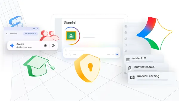 Google’s AI tools help educators support their teaching goals and provide personalized experiences to help students learn in the way that works best for them — all withi…
 How Gemini helps with homework, meal planning and more, so parents have time to focus on the good stuff.
 Job hunting can be a slog. But with a few Google AI tools, you can simplify the process from start to finish.Career Dreamer: The first step in landing a job is finding o…