Tag Archives: machine learning

Toward Human-Centered Design for ML Frameworks


As machine learning (ML) increasingly impacts diverse stakeholders and social groups, it has become necessary for a broader range of developers — even those without formal ML training — to be able to adapt and apply ML to their own problems. In recent years, there have been many efforts to lower the barrier to machine learning, by abstracting complex model behavior into higher-level APIs. For instance, Google has been developing TensorFlow.js, an open-source framework that lets developers write ML code in JavaScript to run directly in web browsers. Despite the abundance of engineering work towards improving APIs, little is known about what non-ML software developers actually need to successfully adopt ML into their daily work practices. Specifically, what do they struggle with when trying modern ML frameworks, and what do they want these frameworks to provide?

In “Software Developers Learning Machine Learning: Motivations, Hurdles, and Desires,” which received a Best Paper Award at the IEEE conference on Visual Languages and Human-Centric Computing (VL/HCC), we share our research on these questions and report the results from a large-scale survey of 645 people who used TensorFlow.js. The vast majority of respondents were software or web developers, who were fairly new to machine learning and usually did not use ML as part of their primary job. We examined the hurdles experienced by developers when using ML frameworks and explored the features and tools that they felt would best assist in their adoption of these frameworks into their programming workflows.

What Do Developers Struggle With Most When Using ML Frameworks?
Interestingly, by far the most common challenge reported by developers was not the lack of a clear API, but rather their own lack of conceptual understanding of ML, which hindered their ability to successfully use ML frameworks. These hurdles ranged from the initial stages of picking a good problem to which they could apply TensorFlow.js (e.g., survey respondents reported not knowing “what to apply ML to, where ML succeeds, where it sucks”), to creating the architecture of a neural net (e.g., “how many units [do] I have to put in when adding layers to the model?”) and knowing how to set and tune parameters during model training (e.g., “deciding what optimizers, loss functions to use”). Without a conceptual understanding of how different parameters affect outcomes, developers often felt overwhelmed by the seemingly infinite space of parameters to tune when debugging ML models.

Without sufficient conceptual support, developers also found it hard to transfer lessons learned from “hello world” API tutorials to their own real-world problems. While API tutorials provide syntax for implementing specific models (e.g., classifying MNIST digits), they typically don't provide the underlying conceptual scaffolding necessary to generalize beyond that specific problem.

Developers often attributed these challenges to their own lack of experience in advanced mathematics. Ironically, despite the abundance of non-experts tinkering with ML frameworks nowadays, many felt that ML frameworks were intended for specialists with advanced training in linear algebra and calculus, and thus not meant for general software developers or product managers. This semblance of imposter syndrome may be fueled by the prevalence of esoteric mathematical terminology in API documentation, which may unintentionally give the impression that an advanced math degree is necessary for even practical integration of ML into software projects. Though math training is indeed beneficial, the ability to grasp and apply practical concepts (e.g., a model’s learning rate) to real-world problems does not require an advanced math degree.

What Do Developers Want From ML Frameworks?
Developers who responded to our survey wanted ML frameworks to teach them not only how to use the API, but also the unspoken idioms that would help them to effectively apply the framework to their own problems.

Pre-made Models with Explicit Support for Modification
A common desire was to have access to libraries of canonical ML models, so that they could modify an existing template rather than creating new ones from scratch. Currently, pre-trained models are being made more widely available in many ML platforms, including TensorFlow.js. However, in their current form, these models do not provide explicit support for novice consumption. For example, in our survey, developers reported substantial hurdles transferring and modifying existing model examples to their own use cases. Thus, the provision of pre-made ML models should also be coupled with explicit support for modification.

Synthesize ML Best Practices into Just-in-Time Hints
Developers also wished frameworks could provide ML best practices, i.e., practical tips and tricks that they could use when designing or debugging models. While ML experts may acquire heuristics and go-to strategies through years of dedicated trial and error, the mere decision overhead of “which parameter should I try tuning first?” can be overwhelming for developers who aren't ML experts. To help narrow this broad space of decision possibilities, ML frameworks could embed tips on best practices directly into the programming workflow. Currently, visualizations like TensorBoard and tfjs-vis make it possible to help see what's going on inside of their models.

Coupling these with just-in-time strategic pointers, such as whether to adapt a pre-trained model or to build one from scratch, or diagnostic checks, like practical tips to “decrease learning rate” if the model is not converging, could help users acquire and make use of practical strategies. These tips could serve as an intermediate scaffolding layer that helps demystify the math theory underlying ML into developer-friendly terms.

Support for Learning-by-Doing
Finally, even though ML frameworks are not traditional learning platforms, software developers are indeed treating them as lightweight vehicles for learning-by-doing. For example, one survey respondent appreciated when conceptual support was tightly interwoven into the framework, rather than being a separate resource: “...the small code demos that you can edit and run right there. Really helps basic understanding.” Another explained that “I prefer learning by doing, so I would like to see more tutorials, examples” embedded into ML frameworks. Some found it difficult to take a formal online course, and would rather learn in bite-sized pieces through hands-on tinkering: “Due to the rest of life, I have to fit learning into small 5-15 minute blocks.”

Given these desires to learn-by-doing, ML frameworks may need to more clearly distinguish between a spectrum of resources aimed at different levels of expertise. Although many frameworks already have “hello world” tutorials, to properly set expectations these frameworks could more explicitly differentiate between API (syntax-specific) onboarding and ML (conceptual) onboarding.

Looking Forward
Ultimately, as the frontiers of ML are still evolving, providing practical, conceptual tips for software developers and creating a shared reservoir of community-curated best practices can benefit ML experts and novices alike. Hopefully, these research findings pave the way for more user-centric designs of future ML frameworks.

Acknowledgements
This work would not have been possible without Yannick Assogba, Sandeep Gupta, Lauren Hannah-Murphy, Michael Terry, Ann Yuan, Nikhil Thorat, Daniel Smilkov, Martin Wattenberg, Fernanda Viegas, and members of PAIR and TensorFlow.js.

Source: Google AI Blog


Setting Fairness Goals with the TensorFlow Constrained Optimization Library


Many technologies that use supervised machine learning are having an increasingly positive impact on peoples’ day-to-day lives, from catching early signs of illnesses to filtering inappropriate content. There is, however, a growing concern that learned models, which generally satisfy the narrow requirement of minimizing a single loss function, may have difficulty addressing broader societal issues such as fairness, which generally requires trading-off multiple competing considerations. Even when such factors are taken into account, these systems may still be incapable of satisfying such complex design requirements, for example that a false negative might be “worse” than a false positive, or that the model being trained should be “similar” to a pre-existing model.

The TensorFlow Constrained Optimization (TFCO) library makes it easy to configure and train machine learning problems based on multiple different metrics (e.g. the precisions on members of certain groups, the true positive rates on residents of certain countries, or the recall rates of cancer diagnoses depending on age and gender). While these metrics are simple conceptually, by offering a user the ability to minimize and constrain arbitrary combinations of them, TFCO makes it easy to formulate and solve many problems of interest to the fairness community in particular (such as equalized odds and predictive parity) and the machine learning community more generally.

How Does TFCO Relate to Our AI Principles?
The release of TFCO puts our AI Principles into action, further helping guide the ethical development and use of AI in research and in practice. By putting TFCO into the hands of developers, we aim to better equip them to identify where their models can be risky and harmful, and to set constraints that ensure their models achieve desirable outcomes.

What Are the Goals?
Borrowing an example from Hardt et al., consider the task of learning a classifier that decides whether a person should receive a loan (a positive prediction) or not (negative), based on a dataset of people who either are able to repay a loan (a positive label), or are not (negative). To set up this problem in TFCO, we would choose an objective function that rewards the model for granting loans to those people who will pay them back, and would also impose fairness constraints that prevent it from unfairly denying loans to certain protected groups of people. In TFCO, the objective to minimize, and the constraints to impose, are represented as algebraic expressions (using normal Python operators) of simple basic rates.

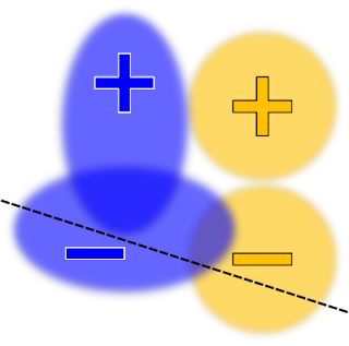
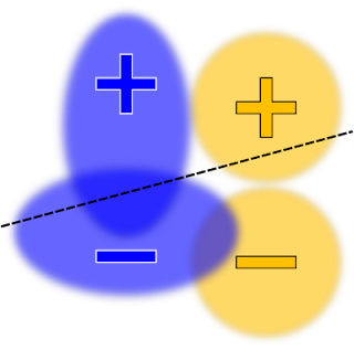
Instructing TFCO to minimize the overall error rate of the learned classifier for a linear model (with no fairness constraints), might yield a decision boundary that looks like this:
Illustration of a binary classification dataset with two protected groups: blue and orange. For ease of visualization, rather than plotting each individual data point, the densities are represented as ovals. The positive and negative signs denote the labels. The decision boundary drawn as a black dashed line separating positive predictions (regions above the line) and negative (regions below the line) labels, chosen to maximize accuracy.
This is a fine classifier, but in certain applications, one might consider it to be unfair. For example, positively-labeled blue examples are much more likely to receive negative predictions than positively-labeled orange examples, violating the “equal opportunity” principle. To correct this, one could add an equal opportunity constraint to the constraint list. The resulting classifier would now look something like this:
Here the decision boundary is chosen to maximize the accuracy, subject to an equal opportunity (or true positive rate) constraint.
How Do I Know What Constraints To Set?
Choosing the “right” constraints depends on the policy goals or requirements of your problem and your users. For this reason, we’ve striven to avoid forcing the user to choose from a curated list of “baked-in” problems. Instead, we’ve tried to maximize flexibility by enabling the user to define an extremely broad range of possible problems, by combining and manipulating simple basic rates.

This flexibility can have a downside: if one isn’t careful, one might attempt to impose contradictory constraints, resulting in a constrained problem with no good solutions. In the context of the above example, one could constrain the false positive rates (FPRs) to be equal, in addition to the true positive rates (TPRs) (i.e., “equalized odds”). However, the potentially contradictory nature of these two sets of constraints, coupled with our requirement for a linear model, could force us to find a solution with extremely low accuracy. For example:
Here the decision boundary is chosen to maximize the accuracy, subject to both the true positive rate and false positive rate constraints.
With an insufficiently-flexible model, either the FPRs of both groups would be equal, but very large (as in the case illustrated above), or the TPRs would be equal, but very small (not shown).

Can It Fail?
The ability to express many fairness goals as rate constraints can help drive progress in the responsible development of machine learning, but it also requires developers to carefully consider the problem they are trying to address. For example, suppose one constrains the training to give equal accuracy for four groups, but that one of those groups is much harder to classify. In this case, it could be that the only way to satisfy the constraints is by decreasing the accuracy of the three easier groups, so that they match the low accuracy of the fourth group. This probably isn’t the desired outcome.

A “safer” alternative is to constrain each group to independently satisfy some absolute metric, for example by requiring each group to achieve at least 75% accuracy. Using such absolute constraints rather than relative constraints will generally keep the groups from dragging each other down. Of course, it is possible to ask for a minimum accuracy that isn’t achievable, so some conscientiousness is still required.

The Curse of Small Sample Sizes
Another common challenge with using constrained optimization is that the groups to which constraints are applied may be under-represented in the dataset. Consequently, the stochastic gradients we compute during training will be very noisy, resulting in slow convergence. In such a scenario, we recommend that users impose the constraints on a separate rebalanced dataset that contains higher proportions from each group, and use the original dataset only to minimize the objective.

For example, in the Wiki toxicity example we provide, we wish to predict if a discussion comment posted on a Wiki talk page is toxic (i.e., contains “rude, disrespectful or unreasonable” content). Only 1.3% of the comments mention a term related to “sexuality”, and a large fraction of these comments are labelled toxic. Hence, training a CNN model without constraints on this dataset leads to the model believing that “sexuality” is a strong indicator of toxicity and results in a high false positive rate for this group. We use TFCO to constrain the false positive rate for four sensitive topics (sexuality, gender identity, religion and race) to be within 2%. To better handle the small group sizes, we use a “re-balanced” dataset to enforce the constraints and the original dataset only to minimize the objective. As shown below, the constrained model is able to significantly lower the false positive rates on the four topic groups, while maintaining almost the same accuracy as the unconstrained model.
Comparison of unconstrained and constrained CNN models for classifying toxic comments on Wiki Talk pages.
Intersectionality – The Challenge of Fine Grained Groups
Overlapping constraints can help create equitable experiences for multiple categories of historically marginalized and minority groups. Extending beyond the above example, we also provide a CelebA example that examines a computer vision model for detecting smiles in images that we wish to perform well across multiple non-mutually-exclusive protected groups. The false positive rate can be an appropriate metric here, since it measures the fraction of images not containing a smiling face that are incorrectly labeled as smiling. By comparing false positive rates based on available age group (young and old) or sex (male and female) categories, we can check for undesirable model bias (i.e., whether images of older people that are smiling are not recognized as such).
Comparison of unconstrained and constrained CNN models for classifying toxic comments on Wiki Talk pages.
Under the Hood
Correctly handling rate constraints is challenging because, being written in terms of counts (e.g., the accuracy rate is the number of correct predictions, divided by the number of examples), the constraint functions are non-differentiable. Algorithmically, TFCO converts a constrained problem into a non-zero-sum two-player game (ALT’19, JMLR’19). This framework can be extended to handle the ranking and regression settings (AAAI’20), more complex metrics such as the F-measure (NeurIPS’19a), or to improve generalization performance (ICML’19).

It is our belief that the TFCO library will be useful in training ML models that take into account the societal and cultural factors necessary to satisfy real-world requirements. Our provided examples (toxicity classification and smile detection) only scratch the surface. We hope that TFCO’s flexibility enables you to handle your problem’s unique requirements.

Acknowledgements
This work was a collaborative effort by the authors of TFCO and associated research papers, including Andrew Cotter, Maya R. Gupta, Heinrich Jiang, Harikrishna Narasimhan, Taman Narayan, Nathan Srebro, Karthik Sridharan, Serena Wang, Blake Woodworth, and Seungil You.

Source: Google AI Blog


Generating Diverse Synthetic Medical Image Data for Training Machine Learning Models


The progress in machine learning (ML) for medical imaging that helps doctors provide better diagnoses has partially been driven by the use of large, meticulously labeled datasets. However, dataset size can be limited in real life due to privacy concerns, low patient volume at partner institutions, or by virtue of studying rare diseases. Moreover, to ensure that ML models generalize well, they need training data that span a range of subgroups, such as skin type, demographics, and imaging devices. Requiring that the size of each combinatorial subgroup (e.g., skin type A with skin condition B, taken by camera C) is also sufficiently large can quickly become impractical.

Today we are happy to share two projects aimed at both improving the diversity of ML training data, and increasing the effective amount of available training data for medical applications. The first project is a configurable method for generation of synthetic skin lesion images in order to improve coverage of rarer skin types and conditions. The second project uses synthetic images as training data to develop an ML model, that can better interpret different biological tissue types across a range of imaging devices.

Generating Diverse Images of Skin Conditions
In “DermGAN: Synthetic Generation of Clinical Skin Images with Pathology”, published in the Machine Learning for Health (ML4H) workshop at NeurIPS 2019, we address problems associated with data diversity in de-identified dermatology images taken by consumer grade cameras. This work addresses (1) the scarcity of imaging data representative of rare skin conditions, and (2) the lower frequency of data covering certain Fitzpatrick skin types. Fitzpatrick skin types range from Type I (“pale white, always burns, never tans”) to Type VI (“darkest brown, never burns”), with datasets generally containing relative few cases at the “boundaries”. In both cases, data scarcity problems are exacerbated by the low signal-to-noise ratio common in the target images, due to the lack of standardized lighting, contrast and field-of-view; variability of the background, such as furniture and clothing; and the fine details of the skin, like hair and wrinkles.

To improve diversity in the skin images, we developed a model, called DermGAN, which generates skin images that exhibit the characteristics of a given pre-specified skin condition, location, and underlying skin color. DermGAN uses an image-to-image translation approach, based on the pix2pix generative adversarial network (GAN) architecture, to learn the underlying mapping from one type of image to another.

DermGAN takes as input a real image and its corresponding, pre-generated semantic map representing the underlying characteristics of the real image (e.g., the skin condition, location of the lesion, and skin type), from which it will generate a new synthetic example with the requested characteristics. The generator is based on the U-Net architecture, but in order to mitigate checkerboard artifacts, the deconvolution layers are replaced with a resizing layer, followed by a convolution. A few customized losses are introduced to improve the quality of the synthetic images, especially within the pathological region. The discriminator component of DermGAN is solely used for training, whereas the generator is evaluated both visually and for use in augmenting the training dataset for a skin condition classifier.
Overview of the generator component of DermGAN. The model takes an RGB semantic map (red box) annotated with the skin condition's size and location (smaller orange rectangle), and outputs a realistic skin image. Colored boxes represent various neural network layers, such as convolutions and ReLU; the skip connections resemble the U-Net and enable information to be propagated at the appropriate scales.
The top row shows generated synthetic examples and the bottom row illustrates real images of basal cell carcinoma (left) and melanocytic nevus (right). More examples can be found in the paper.
In addition to generating visually realistic images, our method enables generation of images of skin conditions or skin types that are more rare and that suffer from a paucity of dermatologic images.
DermGAN can be used to generate skin images (all with melanocytic nevus in this case) with different background skin types (top, by changing the input skin color) and different-sized lesions (bottom, by changing the input lesion size). As the input skin color changes, the lesion changes appearance to match what the lesion would look like on different skin types.
Early results indicated that using the generated images as additional data to train a skin condition classifier may improve performance at detecting rare malignant conditions, such as melanoma. However, more work is needed to explore how best to utilize such generated images to improve accuracy more generally across rarer skin types and conditions.

Generating Pathology Images with Different Labels Across Diverse Scanners
The focus quality of medical images is important for accurate diagnoses. Poor focus quality can trigger both false positives and false negatives, even in otherwise accurate ML-based metastatic breast cancer detection algorithms. Determining whether or not pathology images are in-focus is difficult due to factors such as the complexity of the image acquisition process. Digitized whole-slide images could have poor focus across the entire image, but since they are essentially stitched together from thousands of smaller fields of view, they could also have subregions with different focus properties than the rest of the image. This makes manual screening for focus quality impractical and motivates the desire for an automated approach to detect poorly-focused slides and locate out-of-focus regions. Identifying regions with poor focus might enable re-scanning, or yield opportunities to improve the focusing algorithms used during the scanning process.

In our second project, presented in “Whole-slide image focus quality: Automatic assessment and impact on AI cancer detection”, published in the Journal of Pathology Informatics, we develop a method of evaluating de-identified, large gigapixel pathology images for focus quality issues. This involved training a convolutional neural network on semi-synthetic training data that represent different tissue types and slide scanner optical properties. However, a key barrier towards developing such an ML-based system was the lack of labeled data — focus quality is difficult to grade reliably and labeled datasets were not available. To exacerbate the problem, because focus quality affects minute details of the image, any data collected for a specific scanner may not be representative of other scanners, which may have differences in the physical optical systems, the stitching procedure used to recreate a large pathology image from captured image tiles, white-balance and post-processing algorithms, and more. This led us to develop a novel multi-step system for generating synthetic images that exhibit realistic out-of-focus characteristics.

We deconstructed the process of collecting training data into multiple steps. The first step was to collect images from various scanners and to label in-focus regions. This task is substantially easier than trying to determine the degree to which an image is out of focus, and can be completed by non-experts. Next, we generated synthetic out-of-focus images, inspired by the sequence of events that happen prior to a real out-of-focus image is captured: the optical blurring effect happens first, followed by those photons being collected by a sensor (a process that adds sensor noise), and finally software compression adds noise.

A sequence of images showing step-wise out-of-focus image generation. Images are shown in grayscale to accentuate the difference between steps. First, an in-focus image is collected (a) and a bokeh effect is added to produce a blurry image (b). Next, sensor noise is added to simulate a real image sensor (c), and finally JPEG compression is added to simulate the sharp edges introduced by post-acquisition software processing (d). A real out-of-focus image is shown for comparison (e).
Our study shows that modeling each step is essential for optimal results across multiple scanner types, and remarkably, enabled the detection of spectacular out-of-focus patterns in real data:
An example of a particularly interesting out-of-focus pattern across a biological tissue slice. Areas in blue were recognized by the model to be in-focus, whereas areas highlighted in yellow, orange, or red were more out of focus. The gradation in focus here (represented by concentric circles: a red/orange out-of-focus center surrounded by green/cyan mildly out-of-focus, and then a blue in-focus ring) was caused by a hard “stone” in the center that lifted the surrounding biological tissue.
Implications and Future Outlook
Though the volume of data used to develop ML systems is seen as a fundamental bottleneck, we have presented techniques for generating synthetic data that can be used to improve the diversity of training data for ML models and thereby improve the ability of ML to work well on more diverse datasets. We should caution though that these methods are not appropriate for validation data, so as to avoid bias such as an ML model performing well only on synthetic data. To ensure unbiased, statistically-rigorous evaluation, real data of sufficient volume and diversity will still be needed, though techniques such as inverse probability weighting (for example, as leveraged in our work on ML for chest X-rays) may be useful there. We continue to explore other approaches to more efficiently leverage de-identified data to improve data diversity and reduce the need for large datasets in the development of ML models for healthcare.

Acknowledgements
These projects involved the efforts of multidisciplinary teams of software engineers, researchers, clinicians and cross functional contributors. Key contributors to these projects include Timo Kohlberger, Yun Liu, Melissa Moran, Po-Hsuan Cameron Chen, Trissia Brown, Jason Hipp, Craig Mermel, Martin Stumpe, Amirata Ghorbani, Vivek Natarajan, David Coz, and Yuan Liu. The authors would also like to acknowledge Daniel Fenner, Samuel Yang, Susan Huang, Kimberly Kanada, Greg Corrado and Erica Brand for their advice, members of the Google Health dermatology and pathology teams for their support, and Ashwin Kakarla and Shivamohan Reddy Garlapati for their team for image labeling.

Source: Google AI Blog


Learning to See Transparent Objects


Optical 3D range sensors, like RGB-D cameras and LIDAR, have found widespread use in robotics to generate rich and accurate 3D maps of the environment, from self-driving cars to autonomous manipulators. However, despite the ubiquity of these complex robotic systems, transparent objects (like a glass container) can confound even a suite of expensive sensors that are commonly used. This is because optical 3D sensors are driven by algorithms that assume all surfaces are Lambertian, i.e., they reflect light evenly in all directions, resulting in a uniform surface brightness from all viewing angles. However, transparent objects violate this assumption, since their surfaces both refract and reflect light. Hence, most of the depth data from transparent objects are invalid or contain unpredictable noise.
Transparent objects often fail to be detected by optical 3D sensors. Top, Right: For instance, glass bottles do not show up in the 3D depth imagery captured from an Intel® RealSense™ D415 RGB-D camera. Bottom: A 3D visualization via point clouds constructed from the depth image.
Enabling machines to better sense transparent surfaces would not only improve safety, but could also open up a range of new interactions in unstructured applications — from robots handling kitchenware or sorting plastics for recycling, to navigating indoor environments or generating AR visualizations on glass tabletops.

To address this problem, we teamed up with researchers from Synthesis AI and Columbia University to develop ClearGrasp, a machine learning algorithm that is capable of estimating accurate 3D data of transparent objects from RGB-D images. This is made possible by a large-scale synthetic dataset that we are also releasing publicly today. ClearGrasp can work with inputs from any standard RGB-D camera, using deep learning to accurately reconstruct the depth of transparent objects and generalize to completely new objects unseen during training. This in contrast to previous methods, which required prior knowledge of the transparent objects (e.g., their 3D models), often combined with maps of background lighting and camera positions. In this work, we also demonstrate that ClearGrasp can benefit robotic manipulation by incorporating it into our pick and place robot’s control system, where we observe significant improvements in the grasping success rate of transparent plastic objects.
ClearGrasp uses deep learning to recover accurate 3D depth data of transparent surfaces.
A Visual Dataset of Transparent Objects
Massive quantities of data are required to train any effective deep learning model (e.g., ImageNet for vision or Wikipedia for BERT), and ClearGrasp is no exception. Unfortunately, no datasets are available with 3D data of transparent objects. Existing 3D datasets like Matterport3D or ScanNet overlook transparent surfaces, because they require expensive and time-consuming labeling processes.

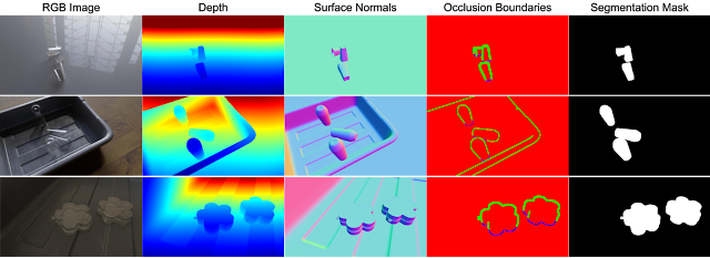
To overcome this issue, we created our own large-scale dataset of transparent objects that contains more than 50,000 photorealistic renders with corresponding surface normals (representing the surface curvature), segmentation masks, edges, and depth, useful for training a variety of 2D and 3D detection tasks. Each image contains up to five transparent objects, either on a flat ground plane or inside a tote, with various backgrounds and lighting.

Some example data of transparent objects from the ClearGrasp synthetic dataset.
We also include a test set of 286 real-world images with corresponding ground truth depth. The real-world images were taken by a painstaking process of replacing each transparent object in the scene with a painted one in the same pose. The images are captured under a number of different indoor lighting conditions, using various cloth and veneer backgrounds and containing random opaque objects scattered around the scene. They contain both known objects, present in the synthetic training set, and novel objects.
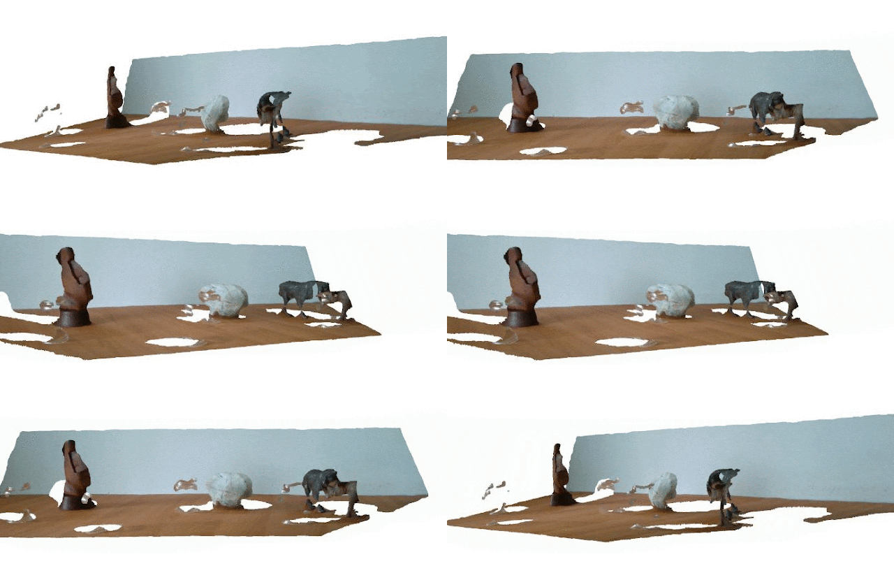
Left: The real-world image capturing setup, Middle: Custom user interface enables precisely replacing each transparent object with a spray-painted duplicate, Right: Example of captured data.
The Challenge
While the distorted view of the background seen through transparent objects confounds typical depth estimation approaches, there are clues that hint at the objects’ shape. Transparent surfaces exhibit specular reflections, which are mirror-like reflections that show up as bright spots in a well-lit environment. Since these visual cues are prominent in RGB images and are influenced primarily by the shape of the objects, convolutional neural networks can use these reflections to infer accurate surface normals, which then can be used for depth estimation.
Specular reflections on transparent objects create distinct features that vary based on the object shape and provide strong visual cues for estimating surface normals.
Most machine learning algorithms try to directly estimate depth from a monocular RGB image. However, monocular depth estimation is an ill-posed task, even for humans. We observed large errors in estimating the depth of flat background surfaces, which compounds the error in depth estimates for the transparent objects resting atop them. Therefore, rather than directly estimating the depth of all geometry, we conjectured that correcting the initial depth estimates from an RGB-D 3D camera is more practical — it would enable us to use the depth from the non-transparent surfaces to inform the depth of transparent surfaces.

The ClearGrasp Algorithm
ClearGrasp uses 3 neural networks: a network to estimate surface normals, one for occlusion boundaries (depth discontinuities), and one that masks transparent objects. The mask is used to remove all pixels belonging to transparent objects, so that the correct depths can be filled in. We then use a global optimization module that starts extending the depth from known surfaces, using the predicted surface normals to guide the shape of the reconstruction, and the predicted occlusion boundaries to maintain the separation between distinct objects.
Overview of our method. The point cloud was generated using the output depth and is colored with its surface normals.
Each of the neural networks was trained on our synthetic dataset and they performed well on real-world transparent objects. However, the surface normal estimations for other surfaces, like walls or fruits, were poor. This is because of the limitations of our synthetic dataset, which contains only transparent objects on a ground plane. To alleviate this issue, we included some real indoor scenes from the Matterport3D and ScanNet datasets in the surface normals training loop. By training on both the in-domain synthetic dataset and out-of-domain real word dataset, the model performed well on all surfaces in our test set.
Surface Normal estimation on real images when trained on a) Matterport3D and ScanNet only (MP+SN), b) our synthetic dataset only, and c) MP+SN as well as our synthetic dataset. Note how the model trained on MP+SN fails to detect the transparent objects. The model trained on only synthetic data picks up the real plastic bottles remarkably well, but fails for other objects and surfaces. When trained on both, our model gets the best of both worlds.
Results
Overall, our quantitative experiments show that ClearGrasp is able to reconstruct depth for transparent objects with much higher fidelity than alternative methods. Despite being trained on only synthetic transparent objects, we find our models are able to adapt well to the real-world domain — achieving very similar quantitative reconstruction performance on known objects across domains. Our models also generalize well to novel objects with complex shapes never seen before.

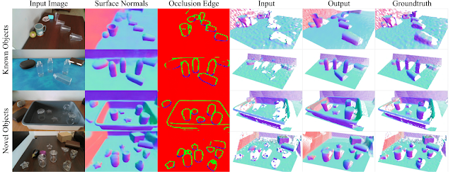
To check the qualitative performance of ClearGrasp, we construct 3D point clouds from the input and output depth images, as shown below (additional examples available on the project webpage). The resulting estimated 3D surfaces have clean and coherent reconstructed shapes — important for applications, such as 3D mapping and 3D object detection — without the jagged noise seen in monocular depth estimation methods. Our models are robust and perform well in challenging conditions, such as identifying transparent objects situated in a patterned background or differentiating between transparent objects partially occluding one another.
Qualitative results on real images. Top two rows: results on known objects. Bottom two rows: results on novel objects. The point clouds, colored with their surface normals, are generated from the corresponding depth images.
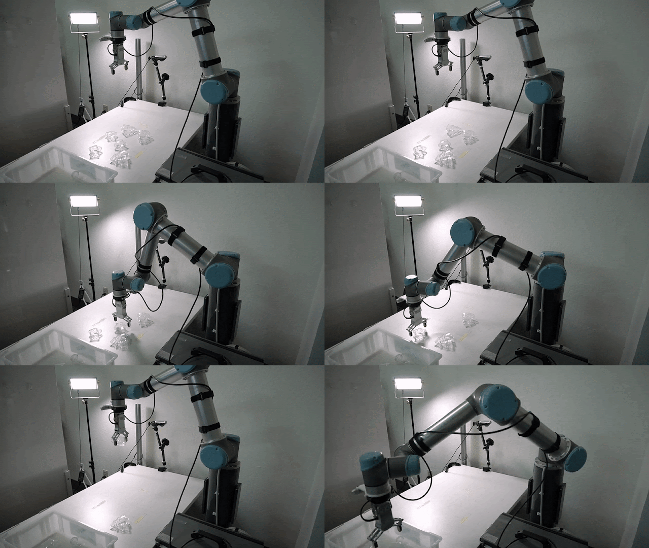
Most importantly, the output depth from ClearGrasp can be directly used as input to state-of-the-art manipulation algorithms that use RGB-D images. By using ClearGrasp’s output depth estimates instead of the raw sensor data, our grasping algorithm on a UR5 robot arm saw significant improvements in the grasping success rates of transparent objects. When using the parallel-jaw gripper, the success rate improved from a baseline of 12% to 74%, and from 64% to 86% with suction.
Manipulation of novel transparent objects using ClearGrasp. Note the challenging conditions: textureless background, complex object shapes and the directional light causing confusing shadows and caustics (the patterns of light that occur when light rays are reflected or refracted from a surface).
Limitations & Future Work
A limitation of our synthetic dataset is that it does not represent accurate caustics, due to the limitations of rendering with traditional path-tracing algorithms. As a result, our models confuse bright caustics coupled with shadows to be independent transparent objects. Despite these drawbacks, our work with ClearGrasp shows that synthetic data remains a viable approach to achieve competent results for learning-based depth reconstruction methods. A promising direction for future work is improving the domain transfer to real-world images by generating renders with physically-correct caustics and surface imperfections such as fingerprints.

With ClearGrasp, we demonstrate that high-quality renders can be used to successfully train models that perform well in the real world. We hope that our dataset will drive further research on data-driven perception algorithms for transparent objects. Download links and more example images can be found on our project website and our GitHub repository.

Acknowledgements
This research was done by Shreeyak Sajjan (Synthesis.ai), Matthew Moore (Synthesis.ai), Mike Pan (Synthesis.ai), Ganesh Nagaraja (Synthesis.ai), Johnny Lee, Andy Zeng, and Shuran Song (Columbia University). We would like to thank Ryan Hickman for managerial support, Ivan Krasin and Stefan Welker for fruitful technical discussions, Cameron (@camfoxmusic) for sharing 3D models of his potion bottles and Sharat Sajjan for helping with web design.

Source: Google AI Blog


TyDi QA: A Multilingual Question Answering Benchmark


Question answering technologies help people on a daily basis — when faced with a question, such as “Is squid ink safe to eat?”, users can ask a voice assistant or type a search and expect to receive an answer. Last year, we released the English-language Natural Questions dataset to the research community to provide a challenge that reflects the needs of real users. However, there are thousands of different languages, and many of those use very different approaches to construct meaning. For example, while English changes words to indicate one object (“book”) versus many (“books”), Arabic also has a third form to indicate if there are two of something ("كتابان", kitaban) beyond just singular ("كتاب", kitab) or plural ("كتب", kutub). In addition, some languages, such as Japanese, do not use spaces between words. Creating machine learning systems that can understand the many ways languages express meaning is challenging, and training such systems requires examples from the diverse the languages to which they will be applied.

To encourage research on multilingual question-answering, today we are releasing TyDi QA, a question answering corpus covering 11 Typologically Diverse languages. Described in our paper, “TyDi QA: A Benchmark for Information-Seeking Question Answering in Typologically Diverse Languages”, our corpus is inspired by typological diversity, a notion that different languages express meaning in structurally different ways. Because we selected a set of languages that are typologically distant from each other for this corpus, we expect models performing well on this dataset to generalize across a large number of the languages in the world.

A Typologically Diverse Collection of Languages
TyDi QA includes over 200,000 question-answer pairs from 11 languages representing a diverse range of linguistic phenomena and data challenges. Many of these languages use non-Latin alphabets, such as Arabic, Bengali, Korean, Russian, Telugu, and Thai. Others form words in complex ways, including Arabic, Finnish, Indonesian, Kiswahili, Russian. Japanese uses four alphabets (shown by the four colors in “24時間でのサーキット周回数”) while the Korean alphabet itself is highly compositional. These languages also range from having much available data on the web (English and Arabic) to very little (Bengali and Kiswahili). We expect that systems that can address these challenges will be successful for a very large number of languages.

Creating Realistic Data
Many early QA datasets used by the research community were created by first showing paragraphs to people and then asking them to write questions based on what could be answered from reading the paragraph. However, since people could see the answer while writing each question, this approach yielded questions that often contained the same words as the answer. As a result, machine learning algorithms trained on such data would favor word matching, oblivious to the more nuanced answers required to satisfy users’ needs.

To construct a more natural dataset, we collected questions from people who wanted an answer, but did not know the answer yet. To inspire questions, we showed people an interesting passage from Wikipedia written in their native language. We then had them ask a question, any question, as long as it was not answered by the passage and they actually wanted to know the answer. This is similar to how your own curiosity might spawn questions about interesting things you see while walking down the street. We encouraged our question writers to let their imaginations run. Does a passage about ice make you think about popsicles in summer? Great! Ask who invented popsicles. Importantly, questions were written directly in each language, not translated, so many questions are unlike those seen in an English-first corpus. One question in Bengali asks, “সফেদা ফল খেতে কেমন?” (What does sapodilla taste like?) Never heard of it? That’s probably because it’s grown much more commonly in India than the U.S.

For each of these questions, we performed a Google Search for the best-matching Wikipedia article in the appropriate language and asked a person to find and highlight the answer within that article. While we expected some interesting divergences between the question and answers when the question writers did not have the answers in front of them, combined with the astonishing breadth of linguistic phenomena in the world’s languages, we found that the situation was even more complex.

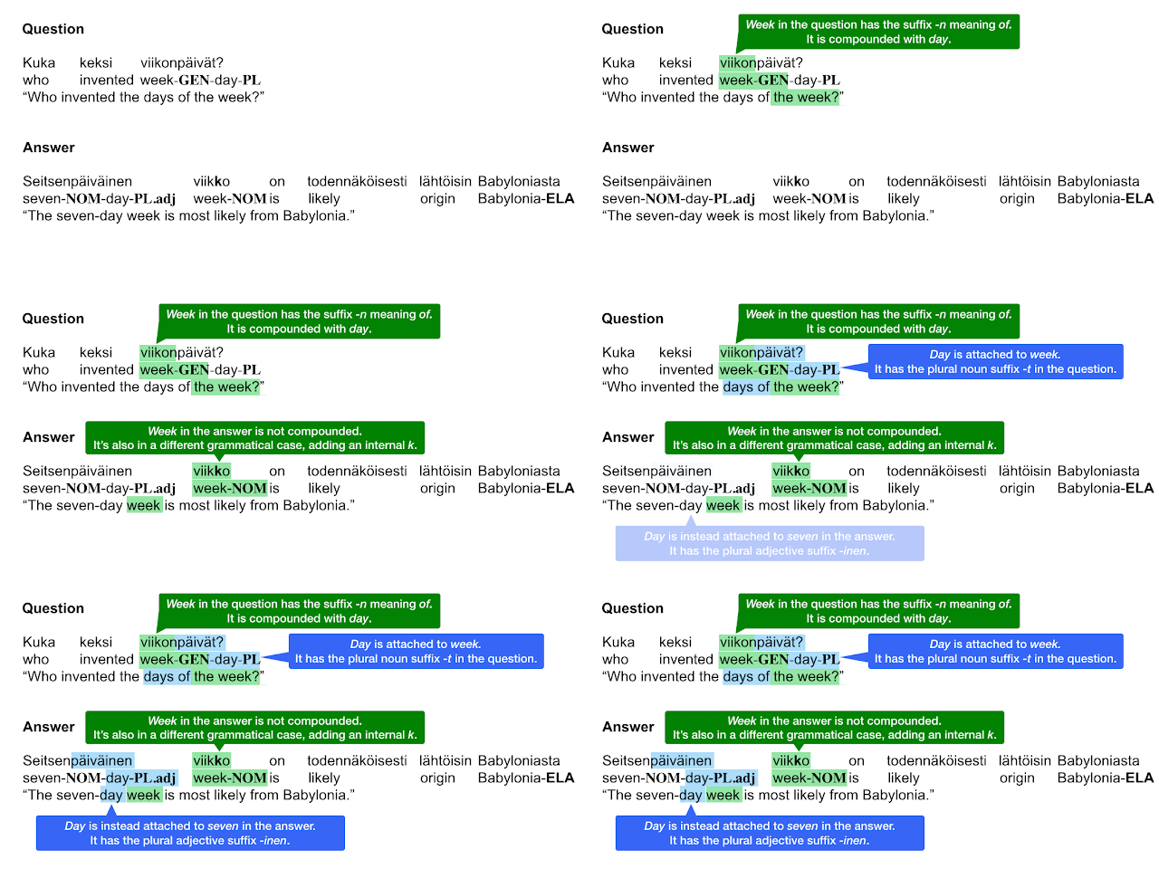
For example, in Finnish, there are fascinating examples in which the words day and week are represented very differently in the question and answer. To be successful in selecting this answer sentence out of an entire Wikipedia article, a system needs to be able to recognize the relationship among the Finnish words viikonpäivät, seitsenpäiväinen, and viikko

Making Progress Together as a Research Community
It is our hope that this dataset will push the research community to innovate in ways that will create more helpful question-answering systems for users around the world. To track the community’s progress, we have established a leaderboard where participants can evaluate the quality of their machine learning systems and are also open-sourcing a question answering system that uses the data. Please visit the challenge website to view the leaderboard and learn more.

Acknowledgements
This dataset is the result of a team of many Googlers including (alphabetically) Dan Garrette, Eunsol Choi, Jennimaria Palomaki, Michael Collins, Tom Kwiatkowski, and Vitaly Nikolaev. The Finnish gloss above is by Jennimaria Palomaki.

Source: Google AI Blog


ML-fairness-gym: A Tool for Exploring Long-Term Impacts of Machine Learning Systems


Machine learning systems have been increasingly deployed to aid in high-impact decision-making, such as determining criminal sentencing, child welfare assessments, who receives medical attention and many other settings. Understanding whether such systems are fair is crucial, and requires an understanding of models’ short- and long-term effects. Common methods for assessing the fairness of machine learning systems involve evaluating disparities in error metrics on static datasets for various inputs to the system. Indeed, many existing ML fairness toolkits (e.g., AIF360, fairlearn, fairness-indicators, fairness-comparison) provide tools for performing such error-metric based analysis on existing datasets. While this sort of analysis may work for systems in simple environments, there are cases (e.g., systems with active data collection or significant feedback loops) where the context in which the algorithm operates is critical for understanding its impact. In these cases, the fairness of algorithmic decisions ideally would be analyzed with greater consideration for the environmental and temporal context than error metric-based techniques allow.

In order to facilitate algorithmic development with this broader context, we have released ML-fairness-gym, a set of components for building simple simulations that explore potential long-run impacts of deploying machine learning-based decision systems in social environments. In “Fairness is not Static: Deeper Understanding of Long Term Fairness via Simulation Studies” we demonstrate how the ML-fairness-gym can be used to research the long-term effects of automated decision systems on a number of established problems from current machine learning fairness literature.

An Example: The Lending Problem
A classic problem for considering fairness in machine learning systems is the lending problem, as described by Liu et al. This problem is a highly simplified and stylized representation of the lending process, where we focus on a single feedback loop in order to isolate its effects and study it in detail. In this problem formulation, the probability that individual applicants will pay back a loan is a function of their credit score. These applicants also belong to one of an arbitrary number of groups, with their group membership observable by the lending bank.

The groups start with different credit score distributions. The bank is trying to determine a threshold on the credit scores, applied across groups or tailored to each, that best enables the bank to reach its objectives. Applicants with scores higher than the threshold receive loans, and those with lower scores are rejected. When the simulation selects an individual, whether or not they will pay the loan is randomly determined based on their group’s probability of payback. In this example, individuals currently applying for loans may apply for additional loans in the future and thus, by paying back their loan, both their credit score and their group’s average credit score increases. Similarly, if the applicant defaults, the group’s average credit score decreases.

The most effective threshold settings will depend on the bank’s goals. A profit-maximizing bank may set a threshold that maximizes the predicted return, based on the estimated likelihood that applicants will repay their loans. Another bank, seeking to be fair to both groups, may try to implement thresholds that maximize profit while satisfying equality of opportunity, the goal of which is to have equal true positive rates (TPR is also called recall or sensitivity; a measure of what fraction of applicants who would have paid back loans were given a loan). In this scenario, machine learning techniques are employed by the bank to determine the most effective threshold based on loans that have been distributed and their outcomes. However, since these techniques are often focused on short-term objectives, they may have unintended and unfair consequences for different groups.
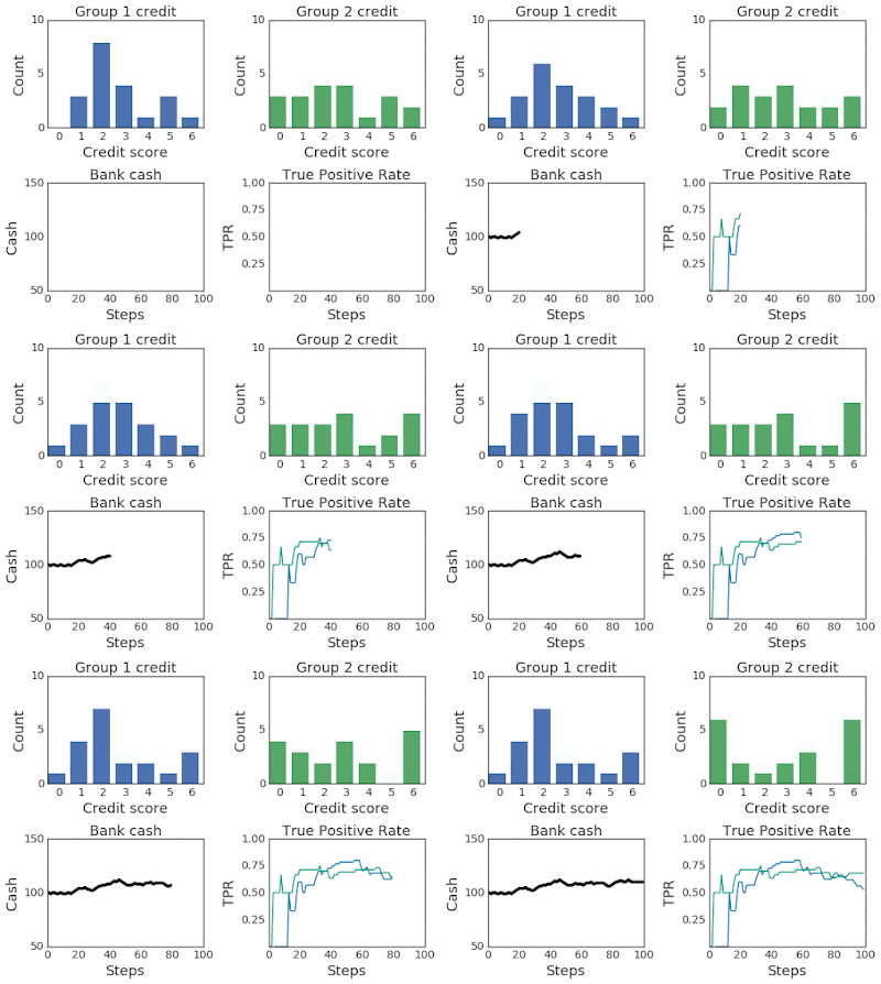
Top:Changing credit score distributions for the two groups over 100 steps of simulation. Bottom: (left) The bank cash and (right) the TPR for group 1 in blue and group 2 in green over the course of the simulation.
Deficiencies in Static Dataset Analysis
A standard practice in machine learning to assess the impact of a scenario like the lending problem is to reserve a portion of the data as a “test set”, and use that to calculate relevant performance metrics. Fairness is then assessed by looking at how those performance metrics differ across salient groups. However, it is well understood that there are two main issues with using test sets like this in systems with feedback. If test sets are generated from existing systems, they may be incomplete or reflect the biases inherent to those systems. In the lending example, a test set could be incomplete because it may only have information on whether an applicant who has been given a loan has defaulted or repaid. Consequently, the dataset may not include individuals for whom loans have not been approved or who have not had access to loans before.

The second issue is that actions informed by the output of the ML system can have effects that may influence their future input. The thresholds determined by the ML system are used to extend loans. Whether people default or repay these loans then affects their future credit score, which then feed back into the ML system.

These issues highlight the shortcomings of assessing fairness in static datasets and motivate the need for analyzing the fairness of algorithms in the context of the dynamic systems in which they are deployed. We created the ML-fairness-gym framework to help ML practitioners bring simulation-based analysis to their ML systems, an approach that has proven effective in many fields for analyzing dynamic systems where closed form analysis is difficult.

ML-fairness-gym as a Simulation Tool for Long-Term Analysis
The ML-fairness-gym simulates sequential decision making using Open AI’s Gym framework. In this framework, agents interact with simulated environments in a loop. At each step, an agent chooses an action that then affects the environment’s state. The environment then reveals an observation that the agent uses to inform its subsequent actions. In this framework, environments model the system and dynamics of the problem and observations serve as data to the agent, which can be encoded as a machine learning system.
Flow chart schematic of the agent-environment interaction loop used in the simulation framework. Agents affect environments via a choice of action. Environments change in response to the action and yield parts of their internal state as an observation. Metrics examine the history of the environment to evaluate outcomes.
In the lending example, the bank acts as the agent. It receives loan applicants, their credit scores and their group membership in the form of observations from the environment, and takes actions in the form of a binary decision to either accept or reject for a loan. The environment then models whether the applicant successfully repays or defaults, and adjusts their credit score accordingly. The ML-fairness-gym simulates the outcomes so that the long-term effects of the bank’s policies on fairness to the applicant population can be assessed.

Fairness Is Not Static: Extending the Analysis to the Long-Term
Since Liu et al.’s original formulation of the lending problem examined only the short-term consequences of the bank’s policies — including short-term profit-maximizing policies (called the max reward agent) and policies subject to an equality of opportunity (EO) constraint — we use the ML-fairness-gym to extend the analysis to the long-term (many steps) via simulation.
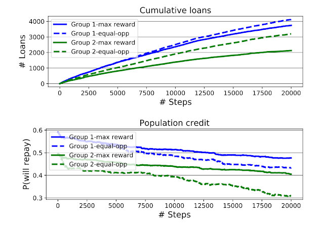
Top: Cumulative loans granted by the max reward and EO agents, stratified by the group identity of the applicant. Bottom: Group average credit (quantified by group-conditional probability of repayment) as the simulation progresses. The EO agent increases access to loans for group 2, but also widens the credit gap between the groups.
Our long-term analysis found two results. First, as found by Liu et al., the equal opportunity agent (EO agent) overlends to the disadvantaged group (group 2, which initially has a lower average credit score) by sometimes applying a lower threshold for the group than would be applied by the max reward agent. This causes the credit scores of group 2 to decrease more than group 1, resulting in a wider credit score gap between the groups than in the simulations with the max reward agent. However, our analysis also found that while group 2 may seem worse off with the EO agent, from looking at the Cumulative loans graph, we see that the disadvantaged group 2 receives significantly more loans from the EO agent. Depending on whether the indicator of welfare is the credit score or total loans received, it could be argued that the EO agent is better or more detrimental to group 2 than the max reward agent.

The second finding is that equal opportunity constraints — enforcing equalized TPR between groups at each step — does not equalize TPR in aggregate over the simulation. This perhaps counterintuitive result can be thought of as an instance of Simpson’s paradox. As seen in the chart below, equal TPR in each of two years does not imply equal TPR in aggregate. This demonstrates how the equality of opportunity metric is difficult to interpret when the underlying population is evolving, and suggests that more careful analysis is necessary to ensure that the ML system is having the desired effects.
An example of Simpson's paradox. TP are the true positive classifications, FN corresponds to the false negative classifications and TPR is the true positive rate. In years 1 and 2, the lender applies a policy that achieves equal TPR between the two groups. The aggregation over both years does not have equal TPR.
Conclusion and Future Work
While we focused on our findings for the lending problem in this blog post, the ML-fairness-gym can be used to tackle a wide variety of fairness problems. Our paper extends the analysis of two other scenarios that have been previously studied in the academic ML fairness literature. The ML-fairness-gym framework is also flexible enough to simulate and explore problems where “fairness” is under-explored. For example, in a supporting paper, “Fair treatment allocations in social networks,” we explore a stylized version of epidemic control, which we call the precision disease control problem, to better understand notions of fairness across individuals and communities in a social network.

We’re excited about the potential of the ML-fairness-gym to help other researchers and machine learning developers better understand the effects that machine learning algorithms have on our society, and to inform the development of more responsible and fair machine learning systems. Find the code and papers in the ML-fairness-gym Github repository.

Source: Google AI Blog


Announcing the Third Workshop and Challenge on Learned Image Compression


With the large amount of media content being downloaded and streamed across the internet, minimizing bandwidth while maintaining quality remains a constant challenge. In 2015, researchers demonstrated that neural network-based image compression could yield significant improvements to image resolution while retaining good quality and high compression speed. Continued advances in compression and bandwidth optimization techniques were stimulated in part by two successful workshops that we hosted at CVPR in 2018 and 2019.

Today, we are excited to announce the Third Workshop and Challenge On Learned Image Compression (CLIC) at CVPR 2020. This workshop challenges researchers to use machine learning, neural networks and other computer vision approaches to increase the quality and lower the bandwidth needed for multimedia transmission. This year’s workshop will also include two challenges: a low-rate image compression challenge and a P-Frame video compression challenge.

Similar to previous years, the goal of the low-rate image compression challenge is to compress an image dataset to 0.15 bits per pixel while maintaining the highest possible quality. Finalists will be selected by measuring their performance against the PSNR and MS-SSIM evaluation metrics. The final ranking will then be determined by a human evaluated rating task.

This year we are also introducing a P-Frame compression track, the first video compression task in this series. In this challenge, participants must first generate a transformation between two adjacent video frames. In the decompression part of the task, participants then use the first frame and their compressed representation to reconstruct the second frame. This challenge will be ranked based solely on the MS-SSIM performance score.

If you are doing research in the field of learned image compression or video compression, we encourage you to participate in CLIC, whether in the two competitions or the paper-only track for publications to be presented at the workshop at CVPR 2020. The validation server is currently available for submissions. The deadline for the final submission of the test set is March 23rd, 2020. For more details on the competition and an up-to-date schedule, please refer to compression.cc. Additional announcements and answers to questions can be found on our Google Groups page.

Acknowledgements
This workshop is being jointly hosted by researchers at Google, Twitter and ETH Zurich. We’d like to thank: George Toderici (Google), Nick Johnston (Google), Johannes Ballé (Google), Eirikur Agustsson (Google), Lucas Theis (Google), Wenzhe Shi (Twitter), Radu Timofte (ETH Zurich) and Fabian Mentzer (ETH Zurich) for their contributions.

Source: Google AI Blog


MediaPipe on the Web

Posted by Michael Hays and Tyler Mullen from the MediaPipe team

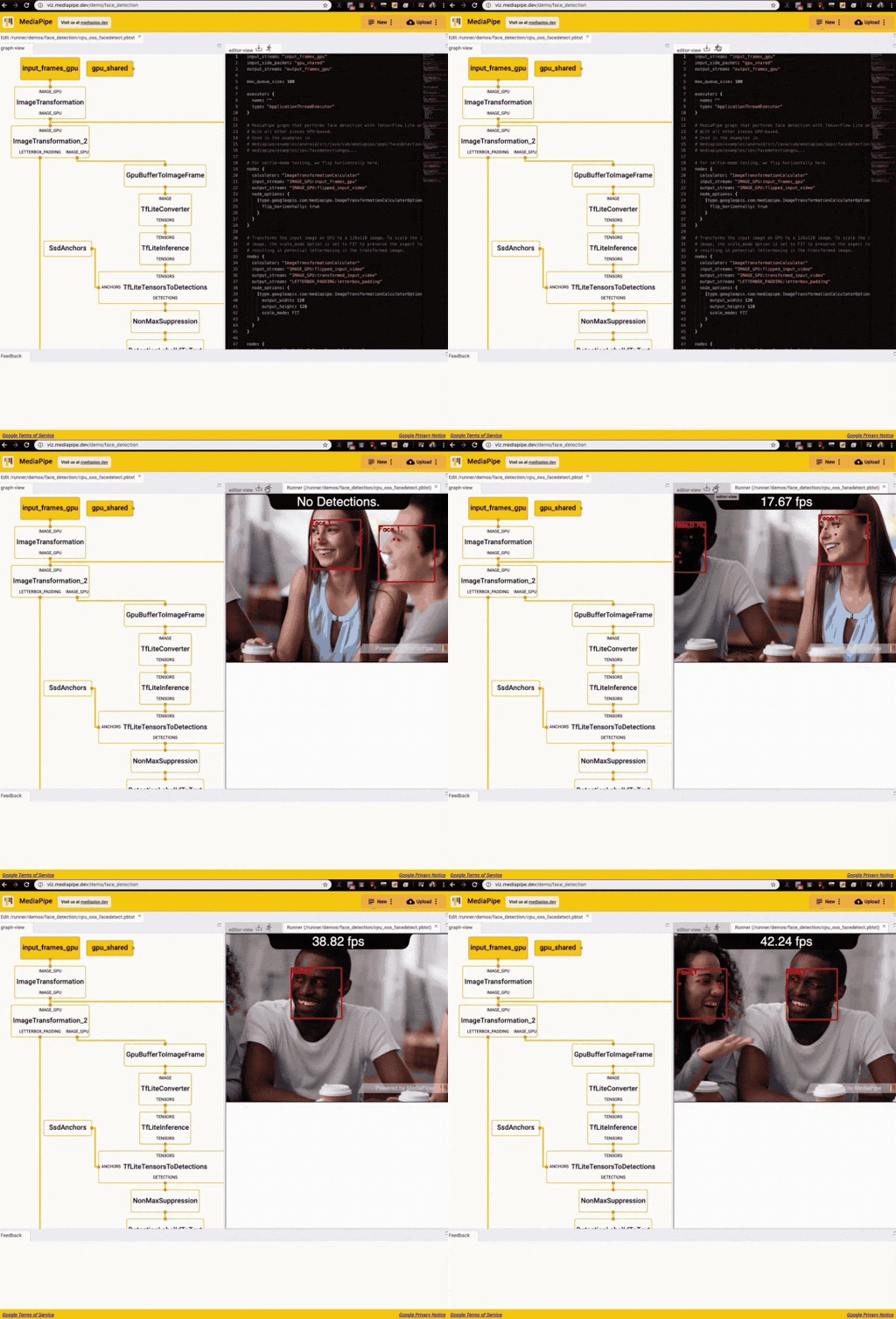
MediaPipe is a framework for building cross-platform multimodal applied ML pipelines. We have previously demonstrated building and running ML pipelines as MediaPipe graphs on mobile (Android, iOS) and on edge devices like Google Coral. In this article, we are excited to present MediaPipe graphs running live in the web browser, enabled by WebAssembly and accelerated by XNNPack ML Inference Library. By integrating this preview functionality into our web-based Visualizer tool, we provide a playground for quickly iterating over a graph design. Since everything runs directly in the browser, video never leaves the user’s computer and each iteration can be immediately tested on a live webcam stream (and soon, arbitrary video).

Running the MediaPipe face detection example in the Visualizer

Figure 1 shows the running of the MediaPipe face detection example in the Visualizer

MediaPipe Visualizer

MediaPipe Visualizer (see Figure 2) is hosted at viz.mediapipe.dev. MediaPipe graphs can be inspected by pasting graph code into the Editor tab or by uploading that graph file into the Visualizer. A user can pan and zoom into the graphical representation of the graph using the mouse and scroll wheel. The graph will also react to changes made within the editor in real time.

MediaPipe Visualizer hosted at https://viz.mediapipe.dev

Figure 2 MediaPipe Visualizer hosted at https://viz.mediapipe.dev

Demos on MediaPipe Visualizer

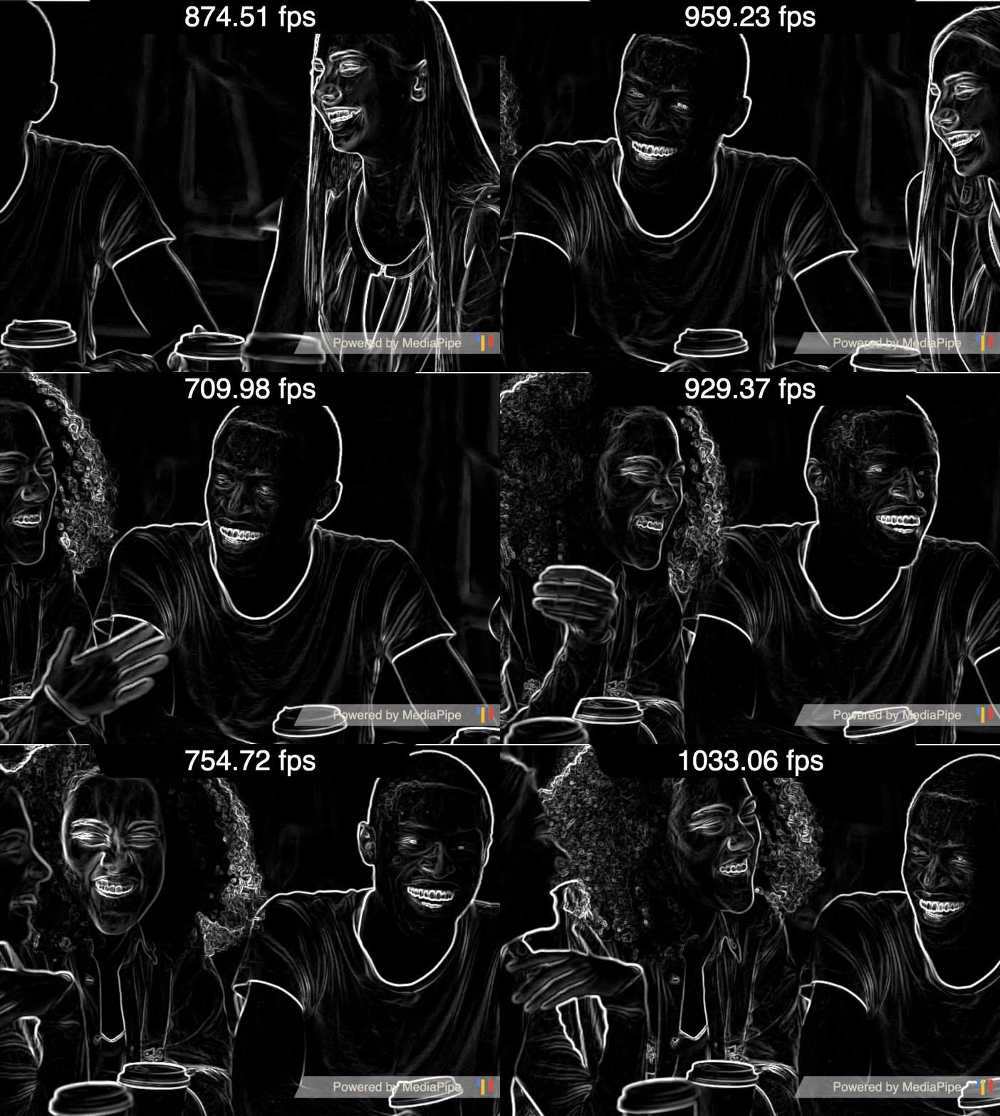
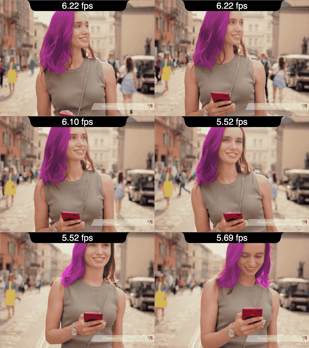
We have created several sample Visualizer demos from existing MediaPipe graph examples. These can be seen within the Visualizer by visiting the following addresses in your Chrome browser:

Edge Detection

Face Detection

Hair Segmentation

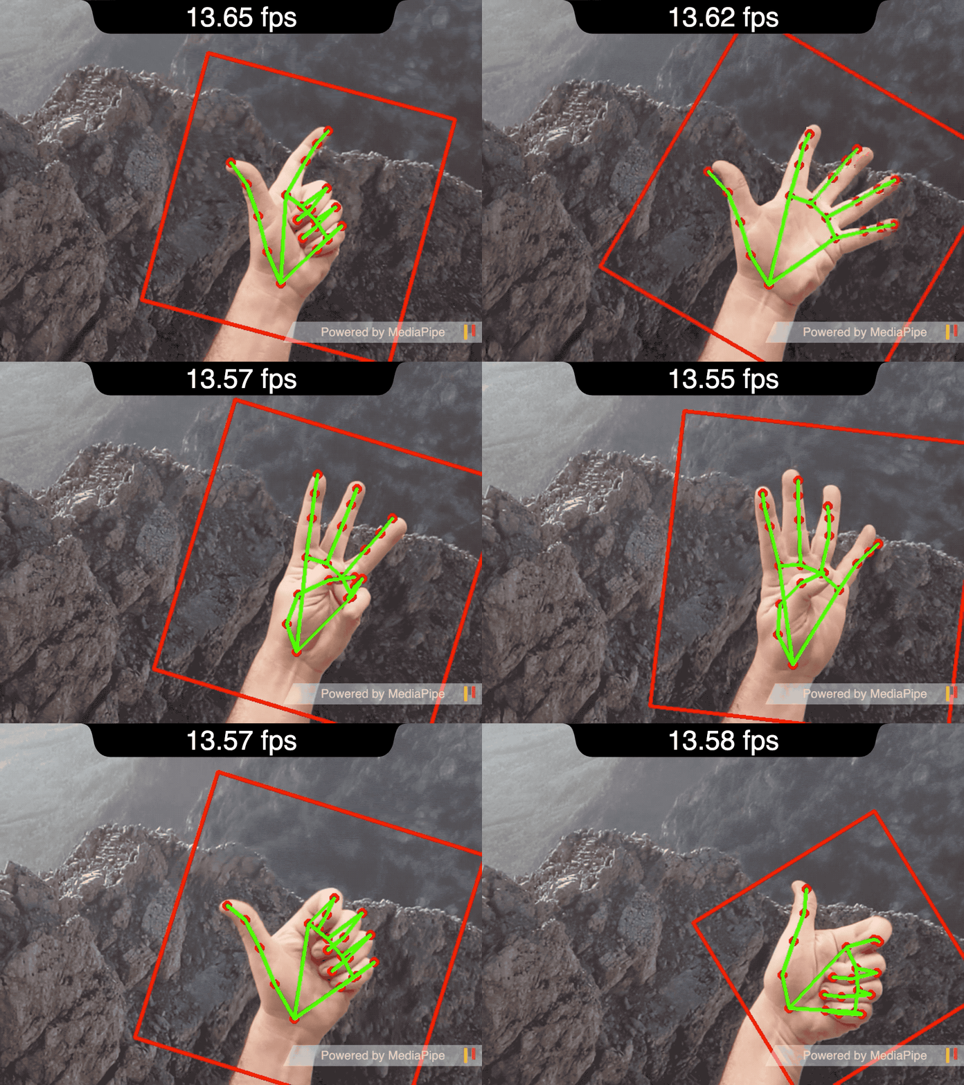
Hand Tracking

Edge detection
Face detection
Hair segmentation
Hand tracking

Each of these demos can be executed within the browser by clicking on the little running man icon at the top of the editor (it will be greyed out if a non-demo workspace is loaded):

This will open a new tab which will run the current graph (this requires a web-cam).

Implementation Details

In order to maximize portability, we use Emscripten to directly compile all of the necessary C++ code into WebAssembly, which is a special form of low-level assembly code designed specifically for web browsers. At runtime, the web browser creates a virtual machine in which it can execute these instructions very quickly, much faster than traditional JavaScript code.

We also created a simple API for all necessary communications back and forth between JavaScript and C++, to allow us to change and interact with the MediaPipe graph directly from JavaScript. For readers familiar with Android development, you can think of this as a similar process to authoring a C++/Java bridge using the Android NDK.

Finally, we packaged up all the requisite demo assets (ML models and auxiliary text/data files) as individual binary data packages, to be loaded at runtime. And for graphics and rendering, we allow MediaPipe to automatically tap directly into WebGL so that most OpenGL-based calculators can “just work” on the web.

Performance

While executing WebAssembly is generally much faster than pure JavaScript, it is also usually much slower than native C++, so we made several optimizations in order to provide a better user experience. We utilize the GPU for image operations when possible, and opt for using the lightest-weight possible versions of all our ML models (giving up some quality for speed). However, since compute shaders are not widely available for web, we cannot easily make use of TensorFlow Lite GPU machine learning inference, and the resulting CPU inference often ends up being a significant performance bottleneck. So to help alleviate this, we automatically augment our “TfLiteInferenceCalculator” by having it use the XNNPack ML Inference Library, which gives us a 2-3x speedup in most of our applications.

Currently, support for web-based MediaPipe has some important limitations:

  • Only calculators in the demo graphs above may be used
  • The user must edit one of the template graphs; they cannot provide their own from scratch
  • The user cannot add or alter assets
  • The executor for the graph must be single-threaded (i.e. ApplicationThreadExecutor)
  • TensorFlow Lite inference on GPU is not supported

We plan to continue to build upon this new platform to provide developers with much more control, removing many if not all of these limitations (e.g. by allowing for dynamic management of assets). Please follow the MediaPipe tag on the Google Developer blog and Google Developer twitter account. (@googledevs)

Acknowledgements

We would like to thank Marat Dukhan, Chuo-Ling Chang, Jianing Wei, Ming Guang Yong, and Matthias Grundmann for contributing to this blog post.

Reformer: The Efficient Transformer


Understanding sequential data — such as language, music or videos — is a challenging task, especially when there is dependence on extensive surrounding context. For example, if a person or an object disappears from view in a video only to re-appear much later, many models will forget how it looked. In the language domain, long short-term memory (LSTM) neural networks cover enough context to translate sentence-by-sentence. In this case, the context window (i.e., the span of data taken into consideration in the translation) covers from dozens to about a hundred words. The more recent Transformer model not only improved performance in sentence-by-sentence translation, but could be used to generate entire Wikipedia articles through multi-document summarization. This is possible because the context window used by Transformer extends to thousands of words. With such a large context window, Transformer could be used for applications beyond text, including pixels or musical notes, enabling it to be used to generate music and images.

However, extending Transformer to even larger context windows runs into limitations. The power of Transformer comes from attention, the process by which it considers all possible pairs of words within the context window to understand the connections between them. So, in the case of a text of 100K words, this would require assessment of 100K x 100K word pairs, or 10 billion pairs for each step, which is impractical. Another problem is with the standard practice of storing the output of each model layer. For applications using large context windows, the memory requirement for storing the output of multiple model layers quickly becomes prohibitively large (from gigabytes with a few layers to terabytes in models with thousands of layers). This means that realistic Transformer models, using numerous layers, can only be used on a few paragraphs of text or generate short pieces of music.

Today, we introduce the Reformer, a Transformer model designed to handle context windows of up to 1 million words, all on a single accelerator and using only 16GB of memory. It combines two crucial techniques to solve the problems of attention and memory allocation that limit Transformer’s application to long context windows. Reformer uses locality-sensitive-hashing (LSH) to reduce the complexity of attending over long sequences and reversible residual layers to more efficiently use the memory available.

The Attention Problem
The first challenge when applying a Transformer model to a very large text sequence is how to handle the attention layer. LSH accomplishes this by computing a hash function that matches similar vectors together, instead of searching through all possible pairs of vectors. For example, in a translation task, where each vector from the first layer of the network represents a word (even larger contexts in subsequent layers), vectors corresponding to the same words in different languages may get the same hash. In the figure below, different colors depict different hashes, with similar words having the same color. When the hashes are assigned, the sequence is rearranged to bring elements with the same hash together and divided into segments (or chunks) to enable parallel processing. Attention is then applied within these much shorter chunks (and their adjoining neighbors to cover the overflow), greatly reducing the computational load.
Locality-sensitive-hashing: Reformer takes in an input sequence of keys, where each key is a vector representing individual words (or pixels, in the case of images) in the first layer and larger contexts in subsequent layers. LSH is applied to the sequence, after which the keys are sorted by their hash and chunked. Attention is applied only within a single chunk and its immediate neighbors.
The Memory Problem
While LSH solves the problem with attention, there is still a memory issue. A single layer of a network often requires up to a few GB of memory and usually fits on a single GPU, so even a model with long sequences could be executed if it only had one layer. But when training a multi-layer model with gradient descent, activations from each layer need to be saved for use in the backward pass. A typical Transformer model has a dozen or more layers, so memory quickly runs out if used to cache values from each of those layers.

The second novel approach implemented in Reformer is to recompute the input of each layer on-demand during back-propagation, rather than storing it in memory. This is accomplished by using reversible layers, where activations from the last layer of the network are used to recover activations from any intermediate layer, by what amounts to running the network in reverse. In a typical residual network, each layer in the stack keeps adding to vectors that pass through the network. Reversible layers, instead, have two sets of activations for each layer. One follows the standard procedure just described and is progressively updated from one layer to the next, but the other captures only the changes to the first. Thus, to run the network in reverse, one simply subtracts the activations applied at each layer.
Reversible layers: (A) In a standard residual network, the activations from each layer are used to update the inputs into the next layer. (B) In a reversible network, two sets of activations are maintained, only one of which is updated after each layer. (C) This approach enables running the network in reverse in order to recover all intermediate values.
Applications of Reformer
The novel application of these two approaches in Reformer makes it highly efficient, enabling it to process text sequences of lengths up to 1 million words on a single accelerator using only 16GB of memory. Since Reformer has such high efficiency, it can be applied directly to data with context windows much larger than virtually all current state-of-the-art text domain datasets. Perhaps Reformer’s ability to deal with such large datasets will stimulate the community to create them.

One area where there is no shortage of large-context data is image generation, so we experiment with the Reformer on images. In this colab, we present examples of how Reformer can be used to “complete” partial images. Starting with the image fragments shown in the top row of the figure below, Reformer can generate full frame images (bottom row), pixel-by-pixel.
Top: Image fragments used as input to Reformer. Bottom: “Completed” full-frame images. Original images are from the Imagenet64 dataset.
While the application of Reformer to imaging and video tasks shows great potential, its application to text is even more exciting. Reformer can process entire novels, all at once and on a single device. Processing the entirety of Crime and Punishment in a single training example is demonstrated in this colab. In the future, when there are more datasets with long-form text to train, techniques such as the Reformer may make it possible to generate long coherent compositions.

Conclusion
We believe Reformer gives the basis for future use of Transformer models, both for long text and applications outside of natural language processing. Following our tradition of doing research in the open, we have already started exploring how to apply it to even longer sequences and how to improve handling of positional encodings. Read the Reformer paper (selected for oral presentation at ICLR 2020), explore our code and develop your own ideas too. Few long-context datasets are widely used in deep learning yet, but in the real world long context is everywhere. Maybe you can find a new application for Reformer — start with this colab and chat with us if you have any problems or questions!

Acknowledgements
This research was conducted by Nikita Kitaev, Łukasz Kaiser and Anselm Levskaya. Additional thanks go to Afroz Mohiuddin, Jonni Kanerva and Piotr Kozakowski for their work on Trax and to the whole JAX team for their support.

Source: Google AI Blog


Using Machine Learning to “Nowcast” Precipitation in High Resolution


The weather can affect a person’s daily routine in both mundane and serious ways, and the precision of forecasting can strongly influence how they deal with it. Weather predictions can inform people about whether they should take a different route to work, if they should reschedule the picnic planned for the weekend, or even if they need to evacuate their homes due to an approaching storm. But making accurate weather predictions can be particularly challenging for localized storms or events that evolve on hourly timescales, such as thunderstorms.

In “Machine Learning for Precipitation Nowcasting from Radar Images,” we are presenting new research into the development of machine learning models for precipitation forecasting that addresses this challenge by making highly localized “physics-free” predictions that apply to the immediate future. A significant advantage of machine learning is that inference is computationally cheap given an already-trained model, allowing forecasts that are nearly instantaneous and in the native high resolution of the input data. This precipitation nowcasting, which focuses on 0-6 hour forecasts, can generate forecasts that have a 1km resolution with a total latency of just 5-10 minutes, including data collection delays, outperforming traditional models, even at these early stages of development.

Moving Beyond Traditional Weather Forecasting
Weather agencies around the world have extensive monitoring facilities. For example, Doppler radar measures precipitation in real-time, weather satellites provide multispectral imaging, ground stations measure wind and precipitation directly, etc. The figure below, which compares false-color composite radar imaging of precipitation over the continental US to cloud cover imaged by geosynchronous satellites, illustrates the need for multi-source weather information. The existence of rain is related to, but not perfectly correlated with, the existence of clouds, so inferring precipitation from satellite images alone is challenging.
Top: Image showing the location of clouds as measured by geosynchronous satellites. Bottom: Radar image showing the location of rain as measured by Doppler radar stations. (Credit: NOAA, NWS, NSSL)
Unfortunately, not all of these measurements are equally present across the globe. For example, radar data comes largely from ground stations and is generally not available over the oceans. Further, coverage varies geographically, and some locations may have poor radar coverage even when they have good satellite coverage.

Even so, there is so much observational data in so many different varieties that forecasting systems struggle to incorporate it all. In the US, remote sensing data collected by the National Oceanic and Atmospheric Administration (NOAA) is now reaching 100 terabytes per day. NOAA uses this data to feed the massive weather forecasting engines that run on supercomputers to provide 1- to 10-day global forecasts. These engines have been developed over the course of the last half century, and are based on numerical methods that directly simulate physical processes, including atmospheric dynamics and numerous effects like thermal radiation, vegetation, lake and ocean effects, and more.

However, the availability of computational resources limits the power of numerical weather prediction in several ways. For example, computational demands limit the spatial resolution to about 5 kilometers, which is not sufficient for resolving weather patterns within urban areas and agricultural land. Numerical methods also take multiple hours to run. If it takes 6 hours to compute a forecast, that allows only 3-4 runs per day and resulting in forecasts based on 6+ hour old data, which limits our knowledge of what is happening right now. By contrast, nowcasting is especially useful for immediate decisions from traffic routing and logistics to evacuation planning.

Radar-to-Radar Forecasting
As a typical example of the type of predictions our system can generate, consider the radar-to-radar forecasting problem: given a sequence of radar images for the past hour, predict what the radar image will be N hours from now, where N typically ranges from 0-6 hours. Since radar data is organized into images, we can pose this prediction as a computer vision problem, inferring the meteorological evolution from the sequence of input images. At these short timescales, the evolution is dominated by two physical processes: advection for the cloud motion, and convection for cloud formation, both of which are significantly affected by local terrain and geography.
Top (left to right): The first three panels show radar images from 60 minutes, 30 minutes, and 0 minutes before now, the point at which a prediction is desired. The right-most panel shows the radar image 60 minutes after now, i.e., the ground truth for a nowcasting prediction. Bottom Left: For comparison, a vector field induced from applying an optical flow (OF) algorithm for modeling advection to the data from the first three panels above. Optical flow is a computer vision method that was developed in the 1940s, and is frequently used to predict short term weather evolution. Bottom Right: An example prediction made by OF. Notice that it tracks the motion of the precipitation in the bottom left corner well, but fails to account for the decaying strength of the storm.
We use a data-driven physics-free approach, meaning that the neural network will learn to approximate the atmospheric physics from the training examples alone, not by incorporating a priori knowledge of how the atmosphere actually works. We treat weather prediction as an image-to-image translation problem, and leverage the current state-of-the-art in image analysis: convolutional neural networks (CNNs).

CNNs are usually composed of a linear sequence of layers, where each layer is a set of operations that transform some input image into a new output image. Often, a layer will change the number of channels and the overall resolution of the image it’s given, in addition to convolving the image with a set of convolutional filters. These filters are themselves small images (for us, they are typically only 3x3, or 5x5). Filters drive much of the power of CNNs, and result in operations like detecting edges, identifying meaningful patterns, etc.

A particularly effective type of CNN is the U-Net. U-Nets have a sequence of layers that are arranged in an encoding phase, in which layers iteratively decrease the resolution of the images passing through them, and then a decoding phase in which the low-dimensional representations of the image created by the encoding phase are expanded back to higher resolutions. The following figure shows all of the layers in our particular U-Net.
(A) The overall structure of our U-NET. Blue boxes correspond to basic CNN layers. Pink boxes correspond to down-sample layers. Green boxes correspond to up-sample layers. Solid lines indicate input connections between layers. Dashed lines indicate long skip connections transversing the encoding and decoding phases of the U-NET. Dotted lines indicate short skip connections for individual layers. (B) The operations within our basic layer. (C) The operations within our down-sample layers. (D) The operations within our up-sample layers.
The input to the U-Net is an image that contains one channel for each multispectral satellite image in the sequence of observations over the last hour. For example, if there were 10 satellite images collected in the last hour, and each of those multispectral images was taken at 10 different wavelengths, then the image input for our model would be an image with 100 channels. For radar-to-radar forecasting, the input is a sequence of 30 radar observations over the past hour, spaced 2 minutes apart, and the output contains the prediction for N hours from now. For our initial work in the US, we trained a network from historical observations over the continental US from the period between 2017 and 2019. The data is split into periods of four weeks, where the first three weeks of each period are used for training and the fourth week is used for evaluation.

Results
We compare our results with three widely used models. First, the High Resolution Rapid Refresh (HRRR) numerical forecast from NOAA. HRRR actually contains predictions for many different weather quantities. We compared our results to their 1-hour total accumulated surface precipitation prediction, as that was their highest quality 1-hour precipitation prediction. Second, an optical flow (OF) algorithm, which attempts to track moving objects through a sequence of images. This latter approach is often applied to weather prediction even though it makes the assumption that overall rain quantities over large areas are constant over the prediction time — an assumption that is clearly violated. Third, the so-called persistence model, is the trivial model in which each location is assumed to be raining in the future at the same rate it is raining now, i.e. the precipitation pattern does not change. That may seem like an overly simplistic model to compare to, but it is common practice given the difficulty of weather prediction.
A visualization of predictions made over the course of roughly one day. Left: The 1-hour HRRR prediction made at the top of each hour, the limit to how often HRRR provides predictions. Center: The ground truth, i.e., what we are trying to predict. Right: The predictions made by our model. Our predictions are every 2 minutes (displayed here every 15 minutes) at roughly 10 times the spatial resolution made by HRRR. Notice that we capture the general motion and general shape of the storm.
We use precision and recall (PR) graphs to compare the models. Since we have direct access to our own classifier, we provide a full PR curve (seen as the blue line in the figure below). However, since we don’t have direct access to the HRRR model, and since neither the persistence model nor OF have the ability to trade-off precision and recall, those models are represented only by individual points. As can be seen, the quality of our neural network forecast outperforms all three of these models (since the blue line is above all of the other model’s results). It is important to note, however, that the HRRR model begins to outperform our current results when the prediction horizon reaches roughly 5 to 6 hours.
Precision and recall (PR) curves comparing our results (solid blue line) with: optical flow (OF), the persistence model, and the HRRR 1-hour prediction. As we do not have direct access to their classifiers, we cannot provide a full PR curve for their results. Left: Predictions for light rain. Right: Predictions for moderate rain.
One of the advantages of the ML method is that predictions are effectively instantaneous, meaning that our forecasts are based on fresh data, while HRRR is hindered by computational latency of 1-3 hours. This leads to better forecasts for computer vision methods for very short term forecasting. In contrast, the numerical model used in HRRR can make better long term predictions, in part because it uses a full 3D physical model — cloud formation is harder to observe from 2D images, and so it is harder for ML methods to learn convective processes. It's possible that combining these two systems, our ML model for rapid forecasts and HRRR for long-term forecasts, could produce better results overall, an idea at the focus of our future work. We're also looking at applying ML directly to 3D observations. Regardless, immediate forecasting is a key tool for real-time planning, facilitating decisions and improving lives.

Acknowledgements
Thanks to Carla Bromberg, Shreya Agrawal, Cenk Gazen, John Burge, Luke Barrington, Aaron Bell, Anand Babu, Stephan Hoyer, Lak Lakshmanan, Brian Williams, Casper Sønderby, Nal Kalchbrenner, Avital Oliver, Tim Salimans, Mostafa Dehghani, Jonathan Heek, Lasse Espeholt, Sella Nevo, Avinatan Hassidim.

Source: Google AI Blog