New sharing dialog for Google Drive, Docs, Sheets, Slides, and Forms

What’s changing 

We’re updating the interface you use to share files from Google Drive, Docs, Sheets, Slides, and Forms on the web. This will replace the previous interface used to share files and manage members of shared drives. These changes will make it easier to share files only with specific people without expanding access beyond what’s needed.

Who’s impacted 

End users

Why it matters 

Sharing files is critical to collaboration. This is especially true now, as more workforces are remote and collaborating on files from different locations. By making it easier to share files with specific people, we hope to improve collaboration while reducing the risk of access by unwanted users. 

Additional details 

We’ve made several changes to the sharing experience. These make it easier to perform common tasks, avoid accidental permission changes, and quickly see who has access to a file. Specifically you may notice:

  • Separated, task-focused interface: The new sharing dialog highlights essential user tasks like sharing a file, changing permissions, and viewing file access. The redesign also visually separates sharing with people and groups from link-sharing. 
  • Quick “copy link” button: We’ve added a “copy link” button to make it easier to get the link without changing link permissions. 
  • Easily see current access: The new interface more clearly shows who currently has access to the item, making it easier to quickly audit and change permissions. 


The new sharing interface for Google Drive and Docs editors files 


The old sharing interface for Google Drive and Docs editors files 

Getting started 


  • Admins: This change will take place by default. There is no admin control for this feature. 
  • End users: This feature will be ON by default. Use our Help Center to learn more about how to share Google Drive files

Rollout pace 


Availability 


  • Available to all G Suite and Drive Enterprise customers, as well as users with personal Google Accounts 

Resources 


Roadmap 


Major Display & Video 360 API v1 Feature Update

Today we’re providing a major feature update to the Display & Video 360 API v1.

This update includes the following features:
Read the release notes for a more detailed list of this new functionality.

You can get started with the Display & Video 360 API and follow our new guides to begin managing your line items and creating new creatives.

If you run into issues or need help using our new functionality, please contact us using our support contact form.

Dev Channel Update for Desktop

The Dev channel has been updated to 84.0.4128.3 for Windows, Mac, and Linux platforms.
A partial list of changes is available in the log. Interested in switching release channels? Find out how. If you find a new issue, please let us know by filing a bug. The community help forum is also a great place to reach out for help or learn about common issues.
Prudhvikumar Bommana Google Chrome

Yet More Google Compute Cluster Trace Data


Google’s Borg cluster management system supports our computational fleet, and underpins almost every Google service. For example, the machines that host the Google Doc used for drafting this post are managed by Borg, as are those that run Google’s cloud computing products. That makes the Borg system, as well as its workload, of great interest to researchers and practitioners.

Eight years ago Google published a 29-day cluster trace — a record of every job submission, scheduling decision, and resource usage data for all the jobs in a Google Borg compute cluster, from May 2011. That trace has enabled a wide range of research on advancing the state of the art for cluster schedulers and cloud computing, and has been used to generate hundreds of analyses and studies. But in the years since the 2011 trace was made available, machines and software have evolved, workloads have changed, and the importance of workload variance has become even clearer.

To help researchers explore these changes themselves, we have released a new trace dataset for the month of May 2019 covering eight Google compute clusters. This new dataset is both larger and more extensive than the 2011 one, and now includes:
  • CPU usage information histograms for each 5 minute period, not just a point sample;
  • information about alloc sets (shared resource reservations used by jobs);
  • job-parent information for master/worker relationships such as MapReduce jobs.
Just like the last trace, the new one focuses on resource requests and usage, and contains no information about end users, their data, or patterns of access to storage systems and other services.

At this time, we are making the trace data available via Google BigQuery so that sophisticated analyses can be performed without requiring local resources. This site provides access instructions and a detailed description of what the traces contain.

A first analysis of differences between the 2011 and 2019 traces appears in this paper.

We hope this data will facilitate even more research into cluster management. Do let us know if you find it useful, publish papers that use it, develop tools that analyze it, or have suggestions for how to improve it.

Acknowledgements
I’d especially like to thank our intern Muhammad Tirmazi, and my colleagues Nan Deng, Md Ehtesam Haque, Zhijing Gene Qin, Steve Hand and Visiting Researcher Adam Barker for doing the heavy lifting of preparing the new trace set.

Source: Google AI Blog


Expanding fact checks on YouTube to the United States

Over the past several years, we've seen more and more people coming to YouTube for news and information. They want to get the latest on an election, to find multiple perspectives on a topic, or to learn about a major breaking news event. More recently, the outbreak of COVID-19 and its spread around the world has reaffirmed how important it is for viewers to get accurate information during fast-moving events. That's why we're continuing to improve the news experience on YouTube, including raising up authoritative sources of information across the site. Today, we’re continuing this work by expanding our fact check information panels — which we launched in Brazil and India last year — to the United States.


The fact check feature expands upon the other ways we raise and connect people with authoritative sources. For example, our Breaking News and Top News shelves help our viewers find information from authoritative sources both on their YouTube homepage and when searching for news topics. In 2018, we introduced information panels that help surface a wide array of contextual information, from links to sources like Encyclopedia Britannica and Wikipedia for topics prone to longstanding misinformation (e.g. "flat earth" theories), or more recently, linking to the WHO, CDC or local health authorities for videos and searches related to COVID-19. We're now using these panels to help address an additional challenge: Misinformation that comes up quickly as part of a fast-moving news cycle, where unfounded claims and uncertainty about facts are common. (For example, a false report that COVID-19 is a bio-weapon.) Our fact check information panels provide fresh context in these situations by highlighting relevant, third-party fact-checked articles above search results for relevant queries, so that our viewers can make their own informed decision about claims made in the news.

There are a few factors that determine whether a fact check information panel will appear for any given search. Most important, there must be a relevant fact check article available from an eligible publisher. And in order to match a viewer’s needs with the information we provide, fact checks will only show when people search for a specific claim. For example, if someone searches for "did a tornado hit Los Angeles," they might see a relevant fact check article, but if they search for a more general query like "tornado," they may not. All fact check articles must also comply with our Community Guidelines, and viewers can send feedback to our team.

Our fact check information panel relies on an open network of third-party publishers and leverages the ClaimReview tagging system. All U.S. publishers are welcome to participate as long as they follow the publicly-available ClaimReview standards and are either a verified signatory of the International Fact-Checking Network’s (IFCN) Code of Principles or are an authoritative publisher. Over a dozen U.S. publishers are participating today, including The Dispatch, FactCheck.org, PolitiFact and The Washington Post Fact Checker, and we encourage more publishers and fact checkers to explore using ClaimReview. In addition to this roll out, YouTube will provide $1M through the Google News Initiative to the IFCN to bolster fact-checking and verification efforts across the world. This follows Google’s efforts to support the ecosystem in the midst of the challenging COVID-19 environment, and we'll be looking for more ways to support the fact check ecosystem in the future.

As always, it will take some time for our systems to fully ramp up. Our systems will become more accurate, and over time, we'll roll this feature out to more countries. We are committed to our responsibility to protect the YouTube community, and expanding our fact check information panels is one of the many steps we are taking to raise up authoritative sources, provide relevant and authoritative context to our users, and continue to reduce the spread of harmful misinformation on YouTube.

Source: YouTube Blog


Stable Channel Update for Desktop

The stable channel has been updated to 81.0.4044.129 for Windows, Mac, and Linux, which will roll out over the coming days/weeks.


A list of all changes is available in the log. Interested in switching release channels? Find out how. If you find a new issue, please let us know by filing a bug. The community help forum is also a great place to reach out for help or learn about common issues.

Security Fixes and Rewards
Note: Access to bug details and links may be kept restricted until a majority of users are updated with a fix. We will also retain restrictions if the bug exists in a third party library that other projects similarly depend on, but haven’t yet fixed.

This update includes 2 security fixes. Below, we highlight fixes that were contributed by external researchers. Please see the Chrome Security Page for more information.

[$10000][1064891] High CVE-2020-6462: Use after free in task scheduling. Reported by Zhe Jin from cdsrc of Qihoo 360 on 2020-03-26
[$TBD][1072983] High CVE-2020-6461: Use after free in storage. Reported by Zhe Jin from cdsrc of Qihoo 360 on 2020-04-21

We would also like to thank all security researchers that worked with us during the development cycle to prevent security bugs from ever reaching the stable channel.

Many of our security bugs are detected using AddressSanitizer, MemorySanitizer, UndefinedBehaviorSanitizer, Control Flow Integrity, libFuzzer, or AFL.


Prudhvikumar Bommana
Google Chrome

Optimizing Multiple Loss Functions with Loss-Conditional Training


In many machine learning applications the performance of a model cannot be summarized by a single number, but instead relies on several qualities, some of which may even be mutually exclusive. For example, a learned image compression model should minimize the compressed image size while maximizing its quality. It is often not possible to simultaneously optimize all the values of interest, either because they are fundamentally in conflict, like the image quality and the compression ratio in the example above, or simply due to the limited model capacity. Hence, in practice one has to decide how to balance the values of interest.
The trade-off between the image quality and the file size in image compression. Ideally both the image distortion and the file size would be minimized, but these two objectives are fundamentally in conflict.
The standard approach to training a model that must balance different properties is to minimize a loss function that is the weighted sum of the terms measuring those properties. For instance, in the case of image compression, the loss function would include two terms, corresponding to the image reconstruction quality and the compression rate. Depending on the coefficients on these terms, training with this loss function results in a model producing image reconstructions that are either more compact or of higher quality.

If one needs to cover different trade-offs between model qualities (e.g. image quality vs compression rate), the standard practice is to train several separate models with different coefficients in the loss function of each. This requires keeping around multiple models both during training and inference, which is very inefficient. However, all of these separate models solve very related problems, suggesting that some information could be shared between them.

In two concurrent papers accepted at ICLR 2020, we propose a simple and broadly applicable approach that avoids the inefficiency of training multiple models for different loss trade-offs and instead uses a single model that covers all of them. In “You Only Train Once: Loss-Conditional Training of Deep Networks”, we give a general formulation of the method and apply it to several tasks, including variational autoencoders and image compression, while in “Adjustable Real-time Style Transfer”, we dive deeper into the application of the method to style transfer.

Loss-Conditional Training
The idea behind our approach is to train a single model that covers all choices of coefficients of the loss terms, instead of training a model for each set of coefficients. We achieve this by (i) training the model on a distribution of losses instead of a single loss function, and (ii) conditioning the model outputs on the vector of coefficients of the loss terms. This way, at inference time the conditioning vector can be varied, allowing us to traverse the space of models corresponding to loss functions with different coefficients.

This training procedure is illustrated in the diagram below for the style transfer task. For each training example, first the loss coefficients are randomly sampled. Then they are used both to condition the main network via the conditioning network and to compute the loss. The whole system is trained jointly end-to-end, i.e., the model parameters are trained concurrently with random sampling of loss functions.
Overview of the method, using stylization as an example. The main stylization network is conditioned on randomly sampled coefficients of the loss function and is trained on a distribution of loss functions, thus learning to model the entire family of loss functions.
The conceptual simplicity of this approach makes it applicable to many problem domains, with only minimal changes to existing code bases. Here we focus on two such applications, image compression and style transfer.

Application: Variable-Rate Image Compression
As a first example application of our approach, we show the results for learned image compression. When compressing an image, a user should be able to choose the desired trade-off between the image quality and the compression rate. Classic image compression algorithms are designed to allow for this choice. Yet, many leading learned compression methods require training a separate model for each such trade-off, which is computationally expensive both at training and at inference time. For problems such as this, where one needs a set of models optimized for different losses, our method offers a simple way to avoid inefficiency and cover all trade-offs with a single model.

We apply the loss-conditional training technique to the learned image compression model of Balle et al. The loss function here consists of two terms, a reconstruction term responsible for the image quality and a compactness term responsible for the compression rate. As illustrated below, our technique allows training a single model covering a wide range of quality-compression tradeoffs.
Compression at different quality levels with a single model. All animations are generated with a single model by varying the conditioning value.
Application: Adjustable Style Transfer
The second application we demonstrate is artistic style transfer, in which one synthesizes an image by merging the content from one image and the style from another. Recent methods allow training deep networks that stylize images in real time and in multiple styles. However, for each given style these methods do not allow the user to have control over the details of the synthesized output, for instance, how much to stylize the image and on which style features to place greater emphasis. If the stylized output is not appealing to the user, they have to train multiple models with different hyper-parameters until they get a favorite stylization.

Our proposed method instead allows training a single model covering a wide range of stylization variants. In this task, we condition the model on a loss function, which has coefficients corresponding to five loss terms, including the content loss and four terms for the stylization loss. Intuitively, the content loss regulates how much the stylized image should be similar to the original content, while the four stylization losses define which style features get carried over to the final stylized image. Below we show the outputs of our single model when varying all these coefficients:
Adjustable style transfer. All stylizations are generated with a single network by varying the conditioning values.
Clearly, the model captures a lot of variation within each style, such as the degree of stylization, the type of elements being added to the image, their exact configuration and locations, and more. More examples can be found on our webpage along with an interactive demo.

Conclusion
We have proposed loss-conditional training, a simple and general method that allows training a single deep network for tasks that would formerly require a large set of separately trained networks. While we have shown its application to image compression and style transfer, many more applications are possible — whenever the loss function has coefficients to be tuned, our method allows training a single model covering a wide range of these coefficients.

Acknowledgements
This blog post covers the work by multiple researchers on the Google Brain team: Mohammad Babaeizadeh, Johannes Balle, Josip Djolonga, Alexey Dosovitskiy, and Golnaz Ghiasi. This blog post would not be possible without crucial contributions from all of them. Images from the MS-COCO dataset and from unsplash.com are used for illustrations.

Source: Google AI Blog


Save power by automatically turning off Google Meet hardware displays

What’s changing

We’ve added a setting in the Admin console to allow you to enable power-saving signaling over HDMI from Google Meet hardware. When enabled, this feature can help you save power by turning off Meet hardware displays when they’re not in use.

Who’s impacted

Admins only

Why you’d use it

Some displays, like those in conference rooms and lobbies, are often left on indefinitely, wasting power and shortening their useful lifespan. This setting allows compatible displays to be turned off automatically after 10 minutes of inactivity.

Displays are automatically turned on 10 minutes before a scheduled meeting or if a user interacts with the touch panel controller.

Additional details

You might need to turn on HDMI-CEC, change other advanced settings, or update the firmware on your display. Consult your displays manual for more information.

Getting started

Admins: This feature will be OFF by default and can be enabled at the organizational unit (OU) level. Visit the Help Center to learn more about turning display power saving on or off for your organization.

End users: There is no end user setting for this feature. Rollout pace This feature is available now for all users.

Availability


  • Available to all G Suite customers

Resources


Roadmap


High refresh rate rendering on Android

Posted by Ady Abraham, Software Engineer

For a long time, phones have had a display that refreshes at 60Hz. Application and game developers could just assume that the refresh rate is 60Hz, frame deadline is 16.6ms, and things would just work. This is no longer the case. New flagship devices are built with higher refresh rate displays, providing smoother animations, lower latency, and an overall nicer user experience. There are also devices that support multiple refresh rates, such as the Pixel 4, which supports both 60Hz and 90Hz.

A 60Hz display refreshes the display content every 16.6ms. This means that an image will be shown for the duration of a multiple of 16.6ms (16.6ms, 33.3ms, 50ms, etc.). A display that supports multiple refresh rates, provides more options to render at different speeds without jitter. For example, a game that cannot sustain 60fps rendering must drop all the way to 30fps on a 60Hz display to remain smooth and stutter free (since the display is limited to present images at a multiple of 16.6ms, the next framerate available is a frame every 33.3ms or 30fps). On a 90Hz device, the same game can drop to 45fps (22.2ms for each frame), providing a much smoother user experience. A device that supports 90Hz and 120Hz can smoothly present content at 120, 90, 60 (120/2), 45(90/2), 40(120/3), 30(90/3), 24(120/5), etc. frames per second.

Rendering at high rates

The higher the rendering rate, the harder it is to sustain that frame rate, simply because there is less time available for the same amount of work. To render at 90Hz, applications only have 11.1ms to produce a frame as opposed to 16.6ms at 60Hz.

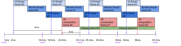
To demonstrate that, let’s take a look at the Android UI rendering pipeline. We can break frame rendering into roughly five pipeline stages:

  1. Application’s UI thread processes input events, calls app’s callbacks, and updates the View hierarchy’s list of recorded drawing commands
  2. Application’s RenderThread issues the recorded commands to the GPU
  3. GPU draws the frame
  4. SurfaceFlinger, which is the system service in charge of displaying the different application windows on the screen, composes the screen and submits the frame to the display HAL
  5. Display presents the frame

The entire pipeline is controlled by the Android Choreographer. The Choreographer is based on the display vertical synchronization (vsync) events, which indicate the time the display starts to scanout the image and update the display pixels. The Choreographer is based on the vsync events but has different wakeup offsets for the application and for SurfaceFlinger. The diagram below illustrates the pipeline on a Pixel 4 device running at 60Hz, where the application is woken up 2ms after the vsync event and SurfaceFlinger is woken up 6ms after the vsync event. This gives 20ms for an app to produce a frame, and 10ms for SurfaceFlinger to compose the screen.

Diagram that illustrates the pipeline on a Pixel 4 device

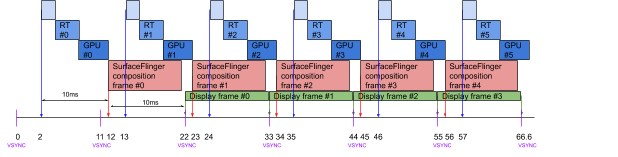
When running at 90Hz, the application is still woken up 2ms after the vsync event. However, SurfaceFlinger is woken up 1ms after the vsync event to have the same 10ms for composing the screen. The app, on the other hand, has just 10ms to render a frame, which is very short.

Diagram of running on a device at 90Hz

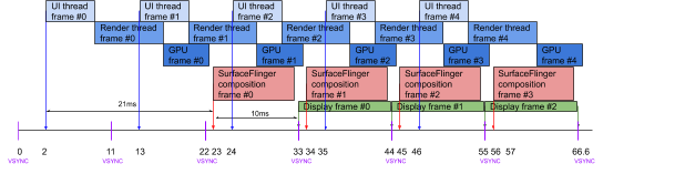
To mitigate that, the UI subsystem in Android is using “render ahead” (which delays a frame presentation while starting it at the same time) to deepen the pipeline and postpone frame presentation by one vsync. This gives the app 21ms to produce a frame, while keeping the throughput at 90Hz.

Diagram app 21ms to produce a frame

Some applications, including most games, have their own custom rendering pipelines. These pipelines might have more or fewer stages, depending on what they are trying to accomplish. In general, as the pipeline becomes deeper, more stages could be performed in parallel, which increases the overall throughput. On the other hand, this can increase the latency of a single frame (the latency will be number_of_pipeline_stages x longest_pipeline_stage). This tradeoff needs to be considered carefully.

Taking advantage of multiple refresh rates

As mentioned above, multiple refresh rates allow a broader range of available rendering rates to be used. This is especially useful for games which can control their rendering speed, and for video players which need to present content at a given rate. For example, to play a 24fps video on a 60Hz display, a 3:2 pulldown algorithm needs to be used, which creates jitter. However, if the device has a display that can present 24fps content natively (24/48/72/120Hz), it will eliminate the need for pulldown and the jitter associated with it.

The refresh rate that the device operates at is controlled by the Android platform. Applications and games can influence the refresh rate via various methods (explained below), but the ultimate decision is made by the platform. This is crucial when more than one app is present on the screen and the platform needs to satisfy all of them. A good example is a 24fps video player. 24Hz might be great for video playback, but it’s awful for responsive UI. A notification animating at only 24Hz feels janky. In situations like this, the platform will set the refresh rate to ensure that the content on the screen looks good.

For this reason, applications may need to know the current device refresh rate. This can be done in the following ways:

Applications can influence the device refresh rate by setting a frame rate on their Window or Surface. This is a new capability introduced in Android 11 and allows the platform to know the rendering intentions of the calling application. Applications can call one of the following methods:

Please refer to the frame rate guide on how to use these APIs.

The system will choose the most appropriate refresh rate based on the frame rate programmed on the Window or Surface.

On Older Android versions (before Android 11) where the setFrameRate API doesn’t exist, applications can still influence the refresh rate by directly setting WindowManager.LayoutParams.preferredDisplayModeId to one of the available modes from Display.getSupportedModes. This approach is discouraged starting with Android 11 since the platform doesn’t know the rendering intention of the app. For example, if a device supports 48Hz, 60Hz and 120Hz and there are two applications present on the screen that call setFrameRate(60, …) and setFrameRate(24, …) respectively, the platform can choose 120Hz and make both applications happy. On the other hand, if those applications used preferredDisplayModeId they would probably set the mode to 60Hz and 48Hz respectively, leaving the platform with no option to set 120Hz. The platform will choose either 60Hz or 48Hz, making one app unhappy.

Takeaways

Refresh rate is not always 60Hz - don’t assume 60Hz and don’t hardcode assumptions based on that historical artifact.

Refresh rate is not always constant - if you care about the refresh rate, you need to register a callback to find out when the refresh rate changes and update your internal data accordingly.

If you are not using the Android UI toolkit and have your own custom renderer, consider changing your rendering pipeline according to the current refresh rate. Deepening the pipeline can be done by setting a presentation timestamp using eglPresentationTimeANDROID on OpenGL or VkPresentTimesInfoGOOGLE on Vulkan. Setting a presentation timestamp indicates to SurfaceFlinger when to present the image. If it is set to a few frames in the future, it will deepen the pipeline by the number of frames it is set to. The Android UI in the example above is setting the present time to frameTimeNanos1 + 2 * vsyncPeriod2

Tell the platform your rendering intentions using the setFrameRate API. The platform will match different requests by selecting the appropriate refresh rate.

Use preferredDisplayModeId only when necessary, either when setFrameRate API is not available or when you need to use a very specific mode.

Lastly, familiarize yourself with the Android Frame Pacing library. This library handles proper frame pacing for your game and uses the methods described above to handle multiple refresh rates.

Notes


  1. frameTimeNanos received from Choreographer 

  2. vsyncPeriod received from Display.getRefreshRate()