Author Archives: Research Blog

Research suggestions at your fingertips with Explore in Docs


Enabling easy access to vast amounts of information across multiple languages and modalities (from text to images to video), computers have become highly influential tools for learning, allowing you to use the world’s information to aid you with your research. However, when researching a topic or writing a term paper, gathering all the information you need from a variety of sources on the Internet can be time-consuming, and at times, a distraction from the writing process.

That’s why we developed algorithms for Explore in Docs, a collaboration between the Coauthor and Apps teams that uses powerful Google infrastructure, best-in-class information retrieval, machine learning, and machine translation technologies to assemble the relevant information and sources for a research paper, all within the document. Explore in Docs suggests relevant content—in the form of topics, images, and snippets —based on the content of the document, allowing the user to focus on critical thinking and idea development.

More than just a Search

Suggesting material that is relevant to the content in a Google Doc is a difficult problem. A naive approach would be to consider the content of a document as a Search query. However, search engines are not designed to accept large blocks of text as queries, so they might truncate the query or focus on the wrong words. So the challenge becomes not only identifying relevant search terms based on the overall content of the document, but additionally providing related topics that may be useful.

To tackle this, the Coauthor team built algorithms that are able to associate external content with topics - entities, abstract concepts - in a document and assign relative importance to each of them. This is accomplished by creating a “target” in a topic vector space that incorporates not only the topics you are writing about but also related topics, creating a variety of search terms that include both. Then, each returned search result (piece of text, image, etc) is embedded in the same vector space and the closest items in that vector space are suggested to the user.

For example, if you’re writing about monarch butterflies, our algorithms find that monarch butterfly and milkweed plant are related to each other. This is done by analyzing the statistics of discourse on the web, collected from hundreds of billions of sentences from billions of webpages across dozens of languages. Note that these two are not semantically close (an insect versus a plant). An example of a set of learned relations is below:
The connection between concepts related to "monarch butterfly", with the thickness of the lines representing the strength of connection, as determined by analysis of discourse on the web. Because this is a discourse graph and not a concept/classification hierarchy, this analysis indicates that "Butterflies & moth" and "Monarch butterfly" are not discussed together as often as "monarch butterfly" and "milkweed".
And because we take the entire document into account while constructing the search request and scoring each candidate piece of text, the resulting suggestions are typically different and more varied than the search snippets users would see if they search the web for each topic individually. By eliminating the need to switch tabs to search, and additionally suggesting new, related topics based on discourse on the web, Explore provides opportunities for learning that users might not discover otherwise - all from the Doc that they’re currently working in!

The information you need, in multiple languages

Cross-lingual predictive search is another key aspect of what we have designed and built. If the relevant material is likely to be in foreign languages, Google searches the web in those languages and translates the selected nuggets into the language of the document.

In the example pictured below, the user begins to type an essay in Docs about Claudia Neto and clicks on the “Explore” button to learn more about her. Explore returns relevant “Topics” and “Images” as well as “Related Research” sourced from multiple websites. Also, Explore suggests Dolores Silva as a related topic since she and Claudia have high mutual information in multilingual web text (statistics collected from more than 10 billion webpages).
Because Swedish ranks high among languages that have significant discourse on Claudia Neto, our algorithms search Swedish content on the Internet for any additional information about her that might not be available on English websites. Before returning information obtained from the Swedish websites, we use Google Translate to render the nugget in the user’s preferred language (in this case, English). Related Research is currently available in 10 languages with more to come in the future.

Explore in Docs is a useful tool that can be used worldwide, in all forms of industry and at all levels of education. Try out the Explore feature the next time you create a document, and check back for more exciting progress from the Coauthor team!

Supercharging Style Transfer


Pastiche. A French word, it designates a work of art that imitates the style of another one (not to be confused with its more humorous Greek cousin, parody). Although it has been used for a long time in visual art, music and literature, pastiche has been getting mass attention lately with online forums dedicated to images that have been modified to be in the style of famous paintings. Using a technique known as style transfer, these images are generated by phone or web apps that allow a user to render their favorite picture in the style of a well known work of art.

Although users have already produced gorgeous pastiches using the current technology, we feel that it could be made even more engaging. Right now, each painting is its own island, so to speak: the user provides a content image, selects an artistic style and gets a pastiche back. But what if one could combine many different styles, exploring unique mixtures of well known artists to create an entirely unique pastiche?

Learning a representation for artistic style

In our recent paper titled “A Learned Representation for Artistic Style”, we introduce a simple method to allow a single deep convolutional style transfer network to learn multiple styles at the same time. The network, having learned multiple styles, is able to do style interpolation, where the pastiche varies smoothly from one style to another. Our method enables style interpolation in real-time as well, allowing this to be applied not only to static images, but also videos.
Credit: awesome dog role played by Google Brain team office dog Picabo.
In the video above, multiple styles are combined in real-time and the resulting style is applied using a single style transfer network. The user is provided with a set of 13 different painting styles and adjusts their relative strengths in the final style via sliders. In this demonstration, the user is an active participant in producing the pastiche.

A Quick History of Style Transfer

While transferring the style of one image to another has existed for nearly 15 years [1] [2], leveraging neural networks to accomplish it is both very recent and very fascinating. In “A Neural Algorithm of Artistic Style” [3], researchers Gatys, Ecker & Bethge introduced a method that uses deep convolutional neural network (CNN) classifiers. The pastiche image is found via optimization: the algorithm looks for an image which elicits the same kind of activations in the CNN’s lower layers - which capture the overall rough aesthetic of the style input (broad brushstrokes, cubist patterns, etc.) - yet produces activations in the higher layers - which capture the things that make the subject recognizable - that are close to those produced by the content image. From some starting point (e.g. random noise, or the content image itself), the pastiche image is progressively refined until these requirements are met.
Content image: The Tübingen Neckarfront by Andreas Praefcke, Style painting: “Head of a Clown”, by Georges Rouault.
The pastiches produced via this algorithm look spectacular:
Figure adapted from L. Gatys et al. "A Neural Algorithm of Artistic Style" (2015). 
This work is considered a breakthrough in the field of deep learning research because it provided the first proof of concept for neural network-based style transfer. Unfortunately this method for stylizing an individual image is computationally demanding. For instance, in the first demos available on the web, one would upload a photo to a server, and then still have plenty of time to go grab a cup of coffee before a result was available.

This process was sped up significantly by subsequent research [4, 5] that recognized that this optimization problem may be recast as an image transformation problem, where one wishes to apply a single, fixed painting style to an arbitrary content image (e.g. a photograph). The problem can then be solved by teaching a feed-forward, deep convolutional neural network to alter a corpus of content images to match the style of a painting. The goal of the trained network is two-fold: maintain the content of the original image while matching the visual style of the painting.

The end result of this was that what once took a few minutes for a single static image, could now be run real time (e.g. applying style transfer to a live video). However, the increase in speed that allowed real-time style transfer came with a cost - a given style transfer network is tied to the style of a single painting, losing some flexibility of the original algorithm, which was not tied to any one style. This means that to build a style transfer system capable of modeling 100 paintings, one has to train and store 100 separate style transfer networks.

Our Contribution: Learning and Combining Multiple Styles

We started from the observation that many artists from the impressionist period employ similar brush stroke techniques and color palettes. Furthermore, painting by say, Monet, are even more visually similar.
Poppy Field (left) and Impression, Sunrise (right) by Claude Monet. Images from Wikipedia
We leveraged this observation in our training of a machine learning system. That is, we trained a single system that is able to capture and generalize across many Monet paintings or even a diverse array of artists across genres. The pastiches produced are qualitatively comparable to those produced in previous work, while originating from the same style transfer network.
Pastiches produced by our single network, trained on 32 varied styles. These pastiches are qualitatively equivalent to those created by single-style networks: Image Credit: (from top to bottom) content photographs by Andreas Praefcke, Rich Niewiroski Jr. and J.-H. Janßen, (from left to right) style paintings by William Glackens, Paul Signac, Georges Rouault, Edvard Munch and Vincent van Gogh.
The technique we developed is simple to implement and is not memory intensive. Furthermore, our network, trained on several artistic styles, permits arbitrary combining multiple painting styles in real-time, as shown in the video above. Here are four styles being combined in different proportions on a photograph of Tübingen:
Unlike previous approaches to fast style transfer, we feel that this method of modeling multiple styles at the same time opens the door to exciting new ways for users to interact with style transfer algorithms, not only allowing the freedom to create new styles based on the mixture of several others, but to do it in real-time. Stay tuned for a future post on the Magenta blog, in which we will describe the algorithm in more detail and release the TensorFlow source code to run this model and demo yourself. We also recommend that you check out Nat & Lo’s fantastic video explanation on the subject of style transfer.

References

[1] Efros, Alexei A., and William T. Freeman. Image quilting for texture synthesis and transfer (2001).

[2] Hertzmann, Aaron, Charles E. Jacobs, Nuria Oliver, Brian Curless, and David H. Salesin. Image analogies (2001).

[3] Gatys, Leon A., Alexander S. Ecker, and Matthias Bethge. A Neural Algorithm of Artistic Style (2015).

[4] Ulyanov, Dmitry, Vadim Lebedev, Andrea Vedaldi, and Victor Lempitsky. Texture Networks: Feed-forward Synthesis of Textures and Stylized Images (2016).

[5] Johnson, Justin, Alexandre Alahi, and Li Fei-Fei. Perceptual Losses for Real-Time Style Transfer and Super-Resolution (2016).


* This work was done during an internship with the Google Brain Team. Vincent is currently a Ph.D. candidate at MILA, Université de Montréal.


Course Builder now supports scheduling, easier customization and more


Over the years, we've learned that there are as many ways to run an online course as there are instructors to run them. Today's release of Course Builder v1.11 has a focus on improved student access controls, easier visual customization and a new course explorer. Additionally, we've added better support for deploying from Windows!

Improved student access controls
A course's availability is often dynamic - sometimes you want to make a course available to everyone all at once, while other times may call for the course to be available to some students before others. Perhaps registration will be available for a while and then the course later becomes read-only. To support these use cases, we've added Student Groups and Calendar Triggers.

  • Student Groups allow you to define which students can see which parts of a course. Want your morning class to see unit 5 and your afternoon class to see unit 6 -- while letting random Internet visitors only see unit 1? Student groups have you covered.
  • Calendar Triggers can be used to update course or content availability automatically at a specific time. For instance, if your course goes live at midnight on Sunday night, you don't need to be at a computer to make it happen. Or, if you want to unlock a new unit every week, you can set up a trigger to automate the process. Read more about calendar triggers and availability.

You can even use these features together. Say you want to start a new group of students through the course every month, giving each access to one new unit per week. Using Student Groups and Calendar Triggers together, you can achieve this cohort-like functionality.

Easier visual customization
In the past, if you wanted to customize Course Builder's student experience beyond a certain point, you needed to be a Python developer. We heard from many web developers that they would like to be able to create their own student-facing pages, too. With this release, Course Builder includes a GraphQL server that allows you to create your own frontend experience, while still letting Course Builder take care of things like user sessions and statefulness.

New course explorer
Large Course Builder partners such as Google's Digital Workshop and NPTEL have many courses and students with diverse needs. To help them, we've completely revamped the Course Explorer page, giving it richer information and interactivity, so your students can find which of your courses they're looking for. You can provide categories and start/end dates, in addition to the course title, abstract and instructor information.
In v1.11, we've added several new highly requested features. Together, they help make Course Builder easier to use and customize, giving you the flexibility to schedule things in advance.

We've come a long way since releasing our first experimental code over 4 years ago, turning Course Builder into a large open-source Google App Engine application with over 5 million student registrations across all Course Builder users. With these latest additions, we consider Course Builder feature complete and fully capable of delivering online learning at any scale. We will continue to provide support and bug fixes for those using the platform.

We hope you’ll enjoy these new features and share how you’re using them in the forum. Keep on learning!

Equality of Opportunity in Machine Learning


As machine learning technology progresses rapidly, there is much interest in understanding its societal impact. A particularly successful branch of machine learning is supervised learning. With enough past data and computational resources, learning algorithms often produce surprisingly effective predictors of future events. To take one hypothetical example: an algorithm could, for example, be used to predict with high accuracy who will pay back their loan. Lenders might then use such a predictor as an aid in deciding who should receive a loan in the first place. Decisions based on machine learning can be both incredibly useful and have a profound impact on our lives.

Even the best predictors make mistakes. Although machine learning aims to minimize the chance of a mistake, how do we prevent certain groups from experiencing a disproportionate share of these mistakes? Consider the case of a group that we have relatively little data on and whose characteristics differ from those of the general population in ways that are relevant to the prediction task. As prediction accuracy is generally correlated with the amount of data available for training, it is likely that incorrect predictions will be more common in this group. A predictor might, for example, end up flagging too many individuals in this group as ‘high risk of default’ even though they pay back their loan. When group membership coincides with a sensitive attribute, such as race, gender, disability, or religion, this situation can lead to unjust or prejudicial outcomes.

Despite the need, a vetted methodology in machine learning for preventing this kind of discrimination based on sensitive attributes has been lacking. A naive approach might require a set of sensitive attributes to be removed from the data before doing anything else with it. This idea of “fairness through unawareness,” however, fails due to the existence of “redundant encodings.” Even if a particular attribute is not present in the data, combinations of other attributes can act as a proxy.

Another common approach, called demographic parity, asks that the prediction must be uncorrelated with the sensitive attribute. This might sound intuitively desirable, but the outcome itself is often correlated with the sensitive attribute. For example, the incidence of heart failure is substantially more common in men than in women. When predicting such a medical condition, it is therefore neither realistic nor desirable to prevent all correlation between the predicted outcome and group membership.

Equal Opportunity

Taking these conceptual difficulties into account, we’ve proposed a methodology for measuring and preventing discrimination based on a set of sensitive attributes. Our framework not only helps to scrutinize predictors to discover possible concerns. We also show how to adjust a given predictor so as to strike a better tradeoff between classification accuracy and non-discrimination if need be.

At the heart of our approach is the idea that individuals who qualify for a desirable outcome should have an equal chance of being correctly classified for this outcome. In our fictional loan example, it means the rate of ‘low risk’ predictions among people who actually pay back their loan should not depend on a sensitive attribute like race or gender. We call this principle equality of opportunity in supervised learning.

When implemented, our framework also improves incentives by shifting the cost of poor predictions from the individual to the decision maker, who can respond by investing in improved prediction accuracy. Perfect predictors always satisfy our notion, showing that the central goal of building more accurate predictors is well aligned with the goal of avoiding discrimination.

Learn more

To explore the ideas in this blog post on your own, our Big Picture team created a beautiful interactive visualization of the different concepts and tradeoffs. So, head on over to their page to learn more.

Once you’ve walked through the demo, please check out the full version of our paper, a joint work with Eric Price (UT Austin) and Nati Srebro (TTI Chicago). We’ll present the paper at this year’s Conference on Neural Information Processing Systems (NIPS) in Barcelona. So, if you’re around, be sure to stop by and chat with one of us.

Our paper is by no means the final word on this important and complex topic. It joins an ongoing conversation with a multidisciplinary focus of research. We hope to inspire future research that will sharpen the discussion of the different achievable tradeoffs surrounding discrimination and machine learning, as well as the development of tools that will help practitioners address these challenges.

Graph-powered Machine Learning at Google


Recently, there have been significant advances in Machine Learning that enable computer systems to solve complex real-world problems. One of those advances is Google’s large scale, graph-based machine learning platform, built by the Expander team in Google Research. A technology that is behind many of the Google products and features you may use everyday, graph-based machine learning is a powerful tool that can be used to power useful features such as reminders in Inbox and smart messaging in Allo, or used in conjunction with deep neural networks to power the latest image recognition system in Google Photos.
Learning with Minimal Supervision

Much of the recent success in deep learning and machine learning, in general, can be attributed to models that demonstrate high predictive capacity when trained on large amounts of labeled data -- often millions of training examples. This is commonly referred to as “supervised learning” since it requires supervision, in the form of labeled data, to train the machine learning systems. (Conversely, some machine learning methods operate directly on raw data without any supervision, a paradigm referred to as unsupervised learning.)

However, the more difficult the task, the harder it is to get sufficient high-quality labeled data. It is often prohibitively labor intensive and time-consuming to collect labeled data for every new problem. This motivated the Expander research team to build new technology for powering machine learning applications at scale and with minimal supervision.

Expander’s technology draws inspiration from how humans learn to generalize and bridge the gap between what they already know (labeled information) and novel, unfamiliar observations (unlabeled information). Known as “semi-supervised” learning, this powerful technique enables us to build systems that can work in situations where training data may be sparse. One of the key advantages to a graph-based semi-supervised machine learning approach is the fact that (a) one models labeled and unlabeled data jointly during learning, leveraging the underlying structure in the data, (b) one can easily combine multiple types of signals (for example, relational information from Knowledge Graph along with raw features) into a single graph representation and learn over them. This is in contrast to other machine learning approaches, such as neural network methods, in which it is typical to first train a system using labeled data with features and then apply the trained system to unlabeled data.

Graph Learning: How It Works

At its core, Expander’s platform combines semi-supervised machine learning with large-scale graph-based learning by building a multi-graph representation of the data with nodes corresponding to objects or concepts and edges connecting concepts that share similarities. The graph typically contains both labeled data (nodes associated with a known output category or label) and unlabeled data (nodes for which no labels were provided). Expander’s framework then performs semi-supervised learning to label all nodes jointly by propagating label information across the graph.

However, this is easier said than done! We have to (1) learn efficiently at scale with minimal supervision (i.e., tiny amount of labeled data), (2) operate over multi-modal data (i.e., heterogeneous representations and various sources of data), and (3) solve challenging prediction tasks (i.e., large, complex output spaces) involving high dimensional data that might be noisy.

One of the primary ingredients in the entire learning process is the graph and choice of connections. Graphs come in all sizes, shapes and can be combined from multiple sources. We have observed that it is often beneficial to learn over multi-graphs that combine information from multiple types of data representations (e.g., image pixels, object categories and chat response messages for PhotoReply in Allo). The Expander team’s graph learning platform automatically generates graphs directly from data based on the inferred or known relationships between data elements. The data can be structured (for example, relational data) or unstructured (for example, sparse or dense feature representations extracted from raw data).

To understand how Expander’s system learns, let us consider an example graph shown below.
There are two types of nodes in the graph: “grey” represents unlabeled data whereas the colored nodes represent labeled data. Relationships between node data is represented via edges and thickness of each edge indicates strength of the connection. We can formulate the semi-supervised learning problem on this toy graph as follows: predict a color (“red” or “blue”) for every node in the graph. Note that the specific choice of graph structure and colors depend on the task. For example, as shown in this research paper we recently published, a graph that we built for the Smart Reply feature in Inbox represents email messages as nodes and colors indicate semantic categories of user responses (e.g., “yes”, “awesome”, “funny”).

The Expander graph learning framework solves this labeling task by treating it as an optimization problem. At the simplest level, it learns a color label assignment for every node in the graph such that neighboring nodes are assigned similar colors depending on the strength of their connection. A naive way to solve this would be to try to learn a label assignment for all nodes at once -- this method does not scale to large graphs. Instead, we can optimize the problem formulation by propagating colors from labeled nodes to their neighbors, and then repeating the process. In each step, an unlabeled node is assigned a label by inspecting color assignments of its neighbors. We can update every node’s label in this manner and iterate until the whole graph is colored. This process is a far more efficient way to optimize the same problem and the sequence of iterations converges to a unique solution in this case. The solution at the end of the graph propagation looks something like this:
Semi-supervised learning on a graph
In practice, we use complex optimization functions defined over the graph structure, which incorporate additional information and constraints for semi-supervised graph learning that can lead to hard, non-convex problems. The real challenge, however, is to scale this efficiently to graphs containing billions of nodes, trillions of edges and for complex tasks involving billions of different label types.

To tackle this challenge, we created an approach outlined in Large Scale Distributed Semi-Supervised Learning Using Streaming Approximation, published last year. It introduces a streaming algorithm to process information propagated from neighboring nodes in a distributed manner that makes it work on very large graphs. In addition, it addresses other practical concerns, notably it guarantees that the space complexity or memory requirements of the system stays constant regardless of the difficulty of the task, i.e., the overall system uses the same amount of memory regardless of whether the number of prediction labels is two (as in the above toy example) or a million or even a billion. This enables wide-ranging applications for natural language understanding, machine perception, user modeling and even joint multimodal learning for tasks involving multiple modalities such as text, image and video inputs.

Language Graphs for Learning Humor

As an example use of graph-based machine learning, consider emotion labeling, a language understanding task in Smart Reply for Inbox, where the goal is to label words occurring in natural language text with their fine-grained emotion categories. A neural network model is first applied to a text corpus to learn word embeddings, i.e., a mathematical vector representation of the meaning of each word. The dense embedding vectors are then used to build a sparse graph where nodes correspond to words and edges represent semantic relationship between them. Edge strength is computed using similarity between embedding vectors — low similarity edges are ignored. We seed the graph with emotion labels known a priori for a few nodes (e.g., laugh is labeled as “funny”) and then apply semi-supervised learning over the graph to discover emotion categories for remaining words (e.g., ROTFL gets labeled as “funny” owing to its multi-hop semantic connection to the word “laugh”).
Learning emotion associations using graph constructed from word embedding vectors
For applications involving large datasets or dense representations that are observed (e.g., pixels from images) or learned using neural networks (e.g., embedding vectors), it is infeasible to compute pairwise similarity between all objects to construct edges in the graph. The Expander team solves this problem by leveraging approximate, linear-time graph construction algorithms.

Graph-based Machine Intelligence in Action

The Expander team’s machine learning system is now being used on massive graphs (containing billions of nodes and trillions of edges) to recognize and understand concepts in natural language, images, videos, and queries, powering Google products for applications like reminders, question answering, 
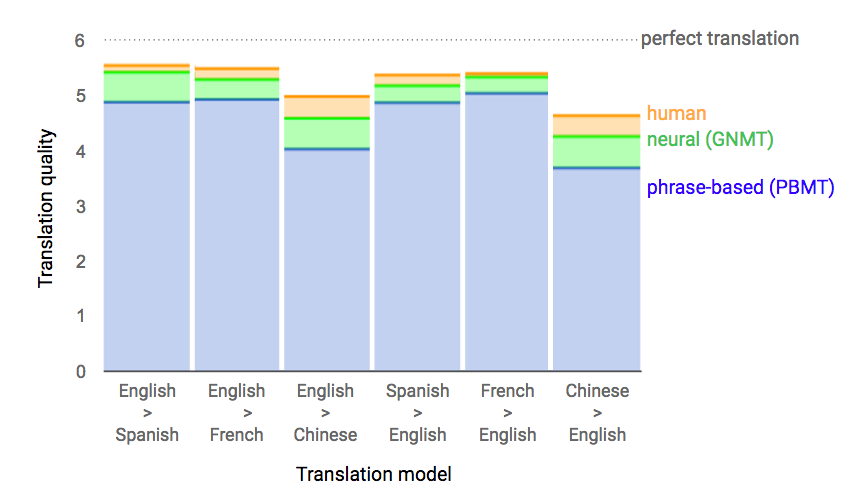
language translation, visual object recognition, dialogue understanding, and more.

We are excited that with the recent release of Allo, millions of chat users are now experiencing smart messaging technology powered by the Expander team’s system for understanding and assisting with chat conversations in multiple languages. Also, this technology isn’t used only for large-scale models in the cloud - as announced this past week, Android Wear has opened up an on-device Smart Reply capability for developers that will provide smart replies for any messaging application. We’re excited to tackle even more challenging Internet-scale problems with Expander in the years to come.

Acknowledgements

We wish to acknowledge the hard work of all the researchers, engineers, product managers, and leaders across Google who helped make this technology a success. In particular, we would like to highlight the efforts of Allan Heydon, Andrei Broder, Andrew Tomkins, Ariel Fuxman, Bo Pang, Dana Movshovitz-Attias, Fritz Obermeyer, Krishnamurthy Viswanathan, Patrick McGregor, Peter Young, Robin Dua, Sujith Ravi and Vivek Ramavajjala.

How Robots Can Acquire New Skills from Their Shared Experience


The ability to learn from experience will likely be a key in enabling robots to help with complex real-world tasks, from assisting the elderly with chores and daily activities, to helping us in offices and hospitals, to performing jobs that are too dangerous or unpleasant for people. However, if each robot must learn its full repertoire of skills for these tasks only from its own experience, it could take far too long to acquire a rich enough range of behaviors to be useful. Could we bridge this gap by making it possible for robots to collectively learn from each other’s experiences?

While machine learning algorithms have made great strides in natural language understanding and speech recognition, the kind of symbolic high-level reasoning that allows people to communicate complex concepts in words remains out of reach for machines. However, robots can instantaneously transmit their experience to other robots over the network - sometimes known as "cloud robotics" - and it is this ability that can let them learn from each other.

This is true even for seemingly simple low-level skills. Humans and animals excel at adaptive motor control that integrates their senses, reflexes, and muscles in a closely coordinated feedback loop. Robots still struggle with these basic skills in the real world, where the variability and complexity of the environment demands well-honed behaviors that are not easily fooled by distractors. If we enable robots to transmit their experiences to each other, could they learn to perform motion skills in close coordination with sensing in realistic environments?

We previously wrote about how multiple robots could pool their experiences to learn a grasping task. Here, we will discuss new experiments that we conducted to investigate three possible approaches for general-purpose skill learning across multiple robots: learning motion skills directly from experience, learning internal models of physics, and learning skills with human assistance. In all three cases, multiple robots shared their experiences to build a common model of the skill. The skills learned by the robots are still relatively simple -- pushing objects and opening doors -- but by learning such skills more quickly and efficiently through collective learning, robots might in the future acquire richer behavioral repertoires that could eventually make it possible for them to assist us in our daily lives.

Learning from raw experience with model-free reinforcement learning.
Perhaps one of the simplest ways for robots to teach each other is to pool information about their successes and failures in the world. Humans and animals acquire many skills by direct trial-and-error learning. During this kind of ‘model-free’ learning -- so called because there is no explicit model of the environment formed -- they explore variations on their existing behavior and then reinforce and exploit the variations that give bigger rewards. In combination with deep neural networks, model-free algorithms have recently proved to be surprisingly effective and have been key to successes with the Atari video game system and playing Go. Having multiple robots allows us to experiment with sharing experiences to speed up this kind of direct learning in the real world.

In these experiments we tasked robots with trying to move their arms to goal locations, or reaching to and opening a door. Each robot has a copy of a neural network that allows it to estimate the value of taking a given action in a given state. By querying this network, the robot can quickly decide what actions might be worth taking in the world. When a robot acts, we add noise to the actions it selects, so the resulting behavior is sometimes a bit better than previously observed, and sometimes a bit worse. This allows each robot to explore different ways of approaching a task. Records of the actions taken by the robots, their behaviors, and the final outcomes are sent back to a central server. The server collects the experiences from all of the robots and uses them to iteratively improve the neural network that estimates value for different states and actions. The model-free algorithms we employed look across both good and bad experiences and distill these into a new network that is better at understanding how action and success are related. Then, at regular intervals, each robot takes a copy of the updated network from the server and begins to act using the information in its new network. Given that this updated network is a bit better at estimating the true value of actions in the world, the robots will produce better behavior. This cycle can then be repeated to continue improving on the task. In the video below, a robot explores the door opening task.
With a few hours of practice, robots sharing their raw experience learn to make reaches to targets, and to open a door by making contact with the handle and pulling. In the case of door opening, the robots learn to deal with the complex physics of the contacts between the hook and the door handle without building an explicit model of the world, as can be seen in the example below:
Learning how the world works by interacting with objects.
Direct trial-and-error reinforcement learning is a great way to learn individual skills. However, humans and animals don’t learn exclusively by trial and error. We also build mental models about our environment and imagine how the world might change in response to our actions.

We can start with the simplest of physical interactions, and have our robots learn the basics of cause and effect from reflecting on their own experiences. In this experiment, we had the robots play with a wide variety of common household objects by randomly prodding and pushing them inside a tabletop bin. The robots again shared their experiences with each other and together built a single predictive model that attempted to forecast what the world might look like in response to their actions. This predictive model can make simple, if slightly blurry, forecasts about future camera images when provided with the current image and a possible sequence of actions that the robot might execute:
Top row: robotic arms interacting with common household items.
Bottom row: Predicted future camera images given an initial image and a sequence of actions.
Once this model is trained, the robots can use it to perform purposeful manipulations, for example based on user commands. In our prototype, a user can command the robot to move a particular object simply by clicking on that object, and then clicking on the point where the object should go:
The robots in this experiment were not told anything about objects or physics: they only see that the command requires a particular pixel to be moved to a particular place. However, because they have seen so many object interactions in their shared past experiences, they can forecast how particular actions will affect particular pixels. In order for such an implicit understanding of physics to emerge, the robots must be provided with a sufficient breadth of experience. This requires either a lot of time, or sharing the combined experiences of many robots. An extended video on this project may be found here.
Learning with the help of humans.
So far, we discussed how robots can learn entirely on their own. However, human guidance is important, not just for telling the robot what to do, but also for helping the robots along. We have a lot of intuition about how various manipulation skills can be performed, and it only seems natural that transferring this intuition to robots can help them learn these skills a lot faster. In the next experiment, we provided each robot with a different door, and guided each of them by hand to show how these doors can be opened. These demonstrations are encoded into a single combined strategy for all robots, called a policy. The policy is a deep neural network which converts camera images to robot actions, and is maintained on a central server. The following video shows the instructor demonstrating the door-opening skill to a robot:
Next, the robots collectively improve this policy through a trial-and-error learning process. Each robot attempts to open its own door using the latest available policy, with some added noise for exploration. These attempts allow each robot to plan a better strategy for opening the door the next time around, and improve the policy accordingly:
Not surprisingly, we find that robots learn more effectively if they are trained on a curriculum of tasks that are gradually increasing in difficulty. In our experiment, each robot starts off by practicing the door-opening skill on a specific position and orientation of the door that the instructor had previously shown it. As it gets better at performing the task, the instructor starts to alter the position and orientation of the door to be just a bit beyond the current capabilities of the policy, but not so difficult that it fails entirely. This allows the robots to gradually increase their skill level over time, and expands the range of situations they can handle. The combination of human-guidance with trial-and-error learning allowed the robots to collectively learn the skill of door-opening in just a couple of hours. Since the robots were trained on doors that look different from each other, the final policy succeeds on a door with a handle that none of the robots had seen before:
In all three of the experiments described above, the ability to communicate and exchange their experiences allows the robots to learn more quickly and effectively. This becomes particularly important when we combine robotic learning with deep learning, as is the case in all of the experiments discussed above. We’ve seen before that deep learning works best when provided with ample training data. For example, the popular ImageNet benchmark uses over 1.5 million labeled examples. While such a quantity of data is not impossible for a single robot to gather over a few years, it is much more efficient to gather the same volume of experience from multiple robots over the course of a few weeks. Besides faster learning times, this approach might benefit from the greater diversity of experience: a real-world deployment might involve multiple robots in different places and different settings, sharing heterogeneous, varied experiences to build a single highly generalizable representation.

Of course, the kinds of behaviors that robots today can learn are still quite limited. Even basic motion skills, such as picking up objects and opening doors, remain in the realm of cutting edge research. In all of these experiments, a human engineer is still needed to tell the robots what they should learn to do by specifying a detailed objective function. However, as algorithms improve and robots are deployed more widely, their ability to share and pool their experiences could be instrumental for enabling them to assist us in our daily lives.

The experiments on learning by trial-and-error were conducted by Shixiang (Shane) Gu and Ethan Holly from the Google Brain team, and Timothy Lillicrap from DeepMind. Work on learning predictive models was conducted by Chelsea Finn from the Google Brain team, and the research on learning from demonstration was conducted by Yevgen Chebotar, Ali Yahya, Adrian Li, and Mrinal Kalakrishnan from X. We would also like to acknowledge contributions by Peter Pastor, Gabriel Dulac-Arnold, and Jon Scholz. Articles about each of the experiments discussed in this blog post can be found below:

Deep Reinforcement Learning for Robotic Manipulation. Shixiang Gu, Ethan Holly, Timothy Lillicrap, Sergey Levine. [video]

Deep Visual Foresight for Planning Robot Motion. Chelsea Finn, Sergey Levine. [video] [data]

Collective Robot Reinforcement Learning with Distributed Asynchronous Guided Policy Search.
Ali Yahya, Adrian Li, Mrinal Kalakrishnan, Yevgen Chebotar, Sergey Levine.  [video]

Path Integral Guided Policy Search. Yevgen Chebotar, Mrinal Kalakrishnan, Ali Yahya, Adrian Li, Stefan Schaal, Sergey Levine. [video]

Introducing the Open Images Dataset


In the last few years, advances in machine learning have enabled Computer Vision to progress rapidly, allowing for systems that can automatically caption images to apps that can create natural language replies in response to shared photos. Much of this progress can be attributed to publicly available image datasets, such as ImageNet and COCO for supervised learning, and YFCC100M for unsupervised learning.

Today, we introduce Open Images, a dataset consisting of ~9 million URLs to images that have been annotated with labels spanning over 6000 categories. We tried to make the dataset as practical as possible: the labels cover more real-life entities than the 1000 ImageNet classes, there are enough images to train a deep neural network from scratch and the images are listed as having a Creative Commons Attribution license*.

The image-level annotations have been populated automatically with a vision model similar to Google Cloud Vision API. For the validation set, we had human raters verify these automated labels to find and remove false positives. On average, each image has about 8 labels assigned. Here are some examples:
Annotated images form the Open Images dataset. Left: Ghost Arches by Kevin Krejci. Right: Some Silverware by J B. Both images used under CC BY 2.0 license
We have trained an Inception v3 model based on Open Images annotations alone, and the model is good enough to be used for fine-tuning applications as well as for other things, like DeepDream or artistic style transfer which require a well developed hierarchy of filters. We hope to improve the quality of the annotations in Open Images the coming months, and therefore the quality of models which can be trained.

The dataset is a product of a collaboration between Google, CMU and Cornell universities, and there are a number of research papers built on top of the Open Images dataset in the works. It is our hope that datasets like Open Images and the recently released YouTube-8M will be useful tools for the machine learning community.


* While we tried to identify images that are licensed under a Creative Commons Attribution license, we make no representations or warranties regarding the license status of each image and you should verify the license for each image yourself.

Image Compression with Neural Networks


Data compression is used nearly everywhere on the internet - the videos you watch online, the images you share, the music you listen to, even the blog you're reading right now. Compression techniques make sharing the content you want quick and efficient. Without data compression, the time and bandwidth costs for getting the information you need, when you need it, would be exorbitant!

In "Full Resolution Image Compression with Recurrent Neural Networks", we expand on our previous research on data compression using neural networks, exploring whether machine learning can provide better results for image compression like it has for image recognition and text summarization. Furthermore, we are releasing our compression model via TensorFlow so you can experiment with compressing your own images with our network.

We introduce an architecture that uses a new variant of the Gated Recurrent Unit (a type of RNN that allows units to save activations and process sequences) called Residual Gated Recurrent Unit (Residual GRU). Our Residual GRU combines existing GRUs with the residual connections introduced in "Deep Residual Learning for Image Recognition" to achieve significant image quality gains for a given compression rate. Instead of using a DCT to generate a new bit representation like many compression schemes in use today, we train two sets of neural networks - one to create the codes from the image (encoder) and another to create the image from the codes (decoder).

Our system works by iteratively refining a reconstruction of the original image, with both the encoder and decoder using Residual GRU layers so that additional information can pass from one iteration to the next. Each iteration adds more bits to the encoding, which allows for a higher quality reconstruction. Conceptually, the network operates as follows:
  1. The initial residual, R[0], corresponds to the original image I: R[0] = I.
  2. Set i=1 for to the first iteration.
  3. Iteration[i] takes R[i-1] as input and runs the encoder and binarizer to compress the image into B[i].
  4. Iteration[i] runs the decoder on B[i] to generate a reconstructed image P[i].
  5. The residual for Iteration[i] is calculated: R[i] = I - P[i].
  6. Set i=i+1 and go to Step 3 (up to the desired number of iterations).
The residual image represents how different the current version of the compressed image is from the original. This image is then given as input to the network with the goal of removing the compression errors from the next version of the compressed image. The compressed image is now represented by the concatenation of B[1] through B[N]. For larger values of N, the decoder gets more information on how to reduce the errors and generate a higher quality reconstruction of the original image.

To understand how this works, consider the following example of the first two iterations of the image compression network, shown in the figures below. We start with an image of a lighthouse. On the first pass through the network, the original image is given as an input (R[0] = I). P[1] is the reconstructed image. The difference between the original image and encoded image is the residual, R[1], which represents the error in the compression.
Left: Original image, I = R[0]. Center: Reconstructed image, P[1]. Right: the residual, R[1], which represents the error introduced by compression.
On the second pass through the network, R[1] is given as the network’s input (see figure below). A higher quality image P[2] is then created. So how does the system recreate such a good image (P[2], center panel below) from the residual R[1]? Because the model uses recurrent nodes with memory, the network saves information from each iteration that it can use in the next one. It learned something about the original image in Iteration[1] that is used along with R[1] to generate a better P[2] from B[2]. Lastly, a new residual, R[2] (right), is generated by subtracting P[2] from the original image. This time the residual is smaller since there are fewer differences between the reconstructed image, and what we started with.
The second pass through the network. Left: R[1] is given as input. Center: A higher quality reconstruction, P[2]. Right: A smaller residual R[2] is generated by subtracting P[2] from the original image.
At each further iteration, the network gains more information about the errors introduced by compression (which is captured by the residual image). If it can use that information to predict the residuals even a little bit, the result is a better reconstruction. Our models are able to make use of the extra bits up to a point. We see diminishing returns, and at some point the representational power of the network is exhausted.

To demonstrate file size and quality differences, we can take a photo of Vash, a Japanese Chin, and generate two compressed images, one JPEG and one Residual GRU. Both images target a perceptual similarity of 0.9 MS-SSIM, a perceptual quality metric that reaches 1.0 for identical images. The image generated by our learned model results in an file 25% smaller than JPEG.
Left: Original image (1419 KB PNG) at ~1.0 MS-SSIM. Center: JPEG (33 KB) at ~0.9 MS-SSIM. Right: Residual GRU (24 KB) at ~0.9 MS-SSIM. This is 25% smaller for a comparable image quality
Taking a look around his nose and mouth, we see that our method doesn’t have the magenta blocks and noise in the middle of the image as seen in JPEG. This is due to the blocking artifacts produced by JPEG, whereas our compression network works on the entire image at once. However, there's a tradeoff -- in our model the details of the whiskers and texture are lost, but the system shows great promise in reducing artifacts.
Left: Original. Center: JPEG. Right: Residual GRU.
While today’s commonly used codecs perform well, our work shows that using neural networks to compress images results in a compression scheme with higher quality and smaller file sizes. To learn more about the details of our research and a comparison of other recurrent architectures, check out our paper. Our future work will focus on even better compression quality and faster models, so stay tuned!

Announcing YouTube-8M: A Large and Diverse Labeled Video Dataset for Video Understanding Research


Many recent breakthroughs in machine learning and machine perception have come from the availability of large labeled datasets, such as ImageNet, which has millions of images labeled with thousands of classes. Their availability has significantly accelerated research in image understanding, for example on detecting and classifying objects in static images.

Video analysis provides even more information for detecting and recognizing objects, and understanding human actions and interactions with the world. Improving video understanding can lead to better video search and discovery, similarly to how image understanding helped re-imagine the photos experience. However, one of the key bottlenecks for further advancements in this area has been the lack of real-world video datasets with the same scale and diversity as image datasets.

Today, we are excited to announce the release of YouTube-8M, a dataset of 8 million YouTube video URLs (representing over 500,000 hours of video), along with video-level labels from a diverse set of 4800 Knowledge Graph entities. This represents a significant increase in scale and diversity compared to existing video datasets. For example, Sports-1M, the largest existing labeled video dataset we are aware of, has around 1 million YouTube videos and 500 sports-specific classes--YouTube-8M represents nearly an order of magnitude increase in both number of videos and classes.
In order to construct a labeled video dataset of this scale, we needed to address two key challenges: (1) video is much more time-consuming to annotate manually than images, and (2) video is very computationally expensive to process and store. To overcome (1), we turned to YouTube and its video annotation system, which identifies relevant Knowledge Graph topics for all public YouTube videos. While these annotations are machine-generated, they incorporate powerful user engagement signals from millions of users as well as video metadata and content analysis. As a result, the quality of these annotations is sufficiently high to be useful for video understanding research and benchmarking purposes.

To ensure the stability and quality of the labeled video dataset, we used only public videos with more than 1000 views, and we constructed a diverse vocabulary of entities, which are visually observable and sufficiently frequent. The vocabulary construction was a combination of frequency analysis, automated filtering, verification by human raters that the entities are visually observable, and grouping into 24 top-level verticals (more details in our technical report). The figures below depict the dataset browser and the distribution of videos along the top-level verticals, and illustrate the dataset’s scale and diversity.
A dataset explorer allows browsing and searching the full vocabulary of Knowledge Graph entities, grouped in 24 top-level verticals, along with corresponding videos. This screenshot depicts a subset of dataset videos annotated with the entity “Guitar”.
The distribution of videos in the top-level verticals illustrates the scope and diversity of the dataset and reflects the natural distribution of popular YouTube videos.
To address (2), we had to overcome the storage and computational resource bottlenecks that researchers face when working with videos. Pursuing video understanding at YouTube-8M’s scale would normally require a petabyte of video storage and dozens of CPU-years worth of processing. To make the dataset useful to researchers and students with limited computational resources, we pre-processed the videos and extracted frame-level features using a state-of-the-art deep learning model--the publicly available Inception-V3 image annotation model trained on ImageNet. These features are extracted at 1 frame-per-second temporal resolution, from 1.9 billion video frames, and are further compressed to fit on a single commodity hard disk (less than 1.5 TB). This makes it possible to download this dataset and train a baseline TensorFlow model at full scale on a single GPU in less than a day!

We believe this dataset can significantly accelerate research on video understanding as it enables researchers and students without access to big data or big machines to do their research at previously unprecedented scale. We hope this dataset will spur exciting new research on video modeling architectures and representation learning, especially approaches that deal effectively with noisy or incomplete labels, transfer learning and domain adaptation. In fact, we show that pre-training models on this dataset and applying / fine-tuning on other external datasets leads to state of the art performance on them (e.g. ActivityNet, Sports-1M). You can read all about our experiments using this dataset, along with more details on how we constructed it, in our technical report.

A Neural Network for Machine Translation, at Production Scale


Ten years ago, we announced the launch of Google Translate, together with the use of Phrase-Based Machine Translation as the key algorithm behind this service. Since then, rapid advances in machine intelligence have improved our speech recognition and image recognition capabilities, but improving machine translation remains a challenging goal.

Today we announce the Google Neural Machine Translation system (GNMT), which utilizes state-of-the-art training techniques to achieve the largest improvements to date for machine translation quality. Our full research results are described in a new technical report we are releasing today: “Google’s Neural Machine Translation System: Bridging the Gap between Human and Machine Translation” [1].

A few years ago we started using Recurrent Neural Networks (RNNs) to directly learn the mapping between an input sequence (e.g. a sentence in one language) to an output sequence (that same sentence in another language) [2]. Whereas Phrase-Based Machine Translation (PBMT) breaks an input sentence into words and phrases to be translated largely independently, Neural Machine Translation (NMT) considers the entire input sentence as a unit for translation.The advantage of this approach is that it requires fewer engineering design choices than previous Phrase-Based translation systems. When it first came out, NMT showed equivalent accuracy with existing Phrase-Based translation systems on modest-sized public benchmark data sets.

Since then, researchers have proposed many techniques to improve NMT, including work on handling rare words by mimicking an external alignment model [3], using attention to align input words and output words [4] and breaking words into smaller units to cope with rare words [5,6]. Despite these improvements, NMT wasn't fast or accurate enough to be used in a production system, such as Google Translate. Our new paper [1] describes how we overcame the many challenges to make NMT work on very large data sets and built a system that is sufficiently fast and accurate enough to provide better translations for Google’s users and services.
Data from side-by-side evaluations, where human raters compare the quality of translations for a given source sentence. Scores range from 0 to 6, with 0 meaning “completely nonsense translation”, and 6 meaning “perfect translation."
The following visualization shows the progression of GNMT as it translates a Chinese sentence to English. First, the network encodes the Chinese words as a list of vectors, where each vector represents the meaning of all words read so far (“Encoder”). Once the entire sentence is read, the decoder begins, generating the English sentence one word at a time (“Decoder”). To generate the translated word at each step, the decoder pays attention to a weighted distribution over the encoded Chinese vectors most relevant to generate the English word (“Attention”; the blue link transparency represents how much the decoder pays attention to an encoded word).
Using human-rated side-by-side comparison as a metric, the GNMT system produces translations that are vastly improved compared to the previous phrase-based production system. GNMT reduces translation errors by more than 55%-85% on several major language pairs measured on sampled sentences from Wikipedia and news websites with the help of bilingual human raters.
An example of a translation produced by our system for an input sentence sampled from a news site. Go here for more examples of translations for input sentences sampled randomly from news sites and books.
In addition to releasing this research paper today, we are announcing the launch of GNMT in production on a notoriously difficult language pair: Chinese to English. The Google Translate mobile and web apps are now using GNMT for 100% of machine translations from Chinese to English—about 18 million translations per day. The production deployment of GNMT was made possible by use of our publicly available machine learning toolkit TensorFlow and our Tensor Processing Units (TPUs), which provide sufficient computational power to deploy these powerful GNMT models while meeting the stringent latency requirements of the Google Translate product. Translating from Chinese to English is one of the more than 10,000 language pairs supported by Google Translate, and we will be working to roll out GNMT to many more of these over the coming months.

Machine translation is by no means solved. GNMT can still make significant errors that a human translator would never make, like dropping words and mistranslating proper names or rare terms, and translating sentences in isolation rather than considering the context of the paragraph or page. There is still a lot of work we can do to serve our users better. However, GNMT represents a significant milestone. We would like to celebrate it with the many researchers and engineers—both within Google and the wider community—who have contributed to this direction of research in the past few years.

Acknowledgements:
We thank members of the Google Brain team and the Google Translate team for the help with the project. We thank Nikhil Thorat and the Big Picture team for the visualization.

References:
[1] Google’s Neural Machine Translation System: Bridging the Gap between Human and Machine Translation, Yonghui Wu, Mike Schuster, Zhifeng Chen, Quoc V. Le, Mohammad Norouzi, Wolfgang Macherey, Maxim Krikun, Yuan Cao, Qin Gao, Klaus Macherey, Jeff Klingner, Apurva Shah, Melvin Johnson, Xiaobing Liu, Łukasz Kaiser, Stephan Gouws, Yoshikiyo Kato, Taku Kudo, Hideto Kazawa, Keith Stevens, George Kurian, Nishant Patil, Wei Wang, Cliff Young, Jason Smith, Jason Riesa, Alex Rudnick, Oriol Vinyals, Greg Corrado, Macduff Hughes, Jeffrey Dean. Technical Report, 2016.
[2] Sequence to Sequence Learning with Neural Networks, Ilya Sutskever, Oriol Vinyals, Quoc V. Le. Advances in Neural Information Processing Systems, 2014.
[3] Addressing the rare word problem in neural machine translation, Minh-Thang Luong, Ilya Sutskever, Quoc V. Le, Oriol Vinyals, and Wojciech Zaremba. Proceedings of the 53th Annual Meeting of the Association for Computational Linguistics, 2015.
[4] Neural Machine Translation by Jointly Learning to Align and Translate, Dzmitry Bahdanau, Kyunghyun Cho, Yoshua Bengio. International Conference on Learning Representations, 2015.
[5] Japanese and Korean voice search, Mike Schuster, and Kaisuke Nakajima. IEEE International Conference on Acoustics, Speech and Signal Processing, 2012.
[6] Neural Machine Translation of Rare Words with Subword Units, Rico Sennrich, Barry Haddow, Alexandra Birch. Proceedings of the 54th Annual Meeting of the Association for Computational Linguistics, 2016.