Tag Archives: Machine Perception

Real-Time 3D Object Detection on Mobile Devices with MediaPipe


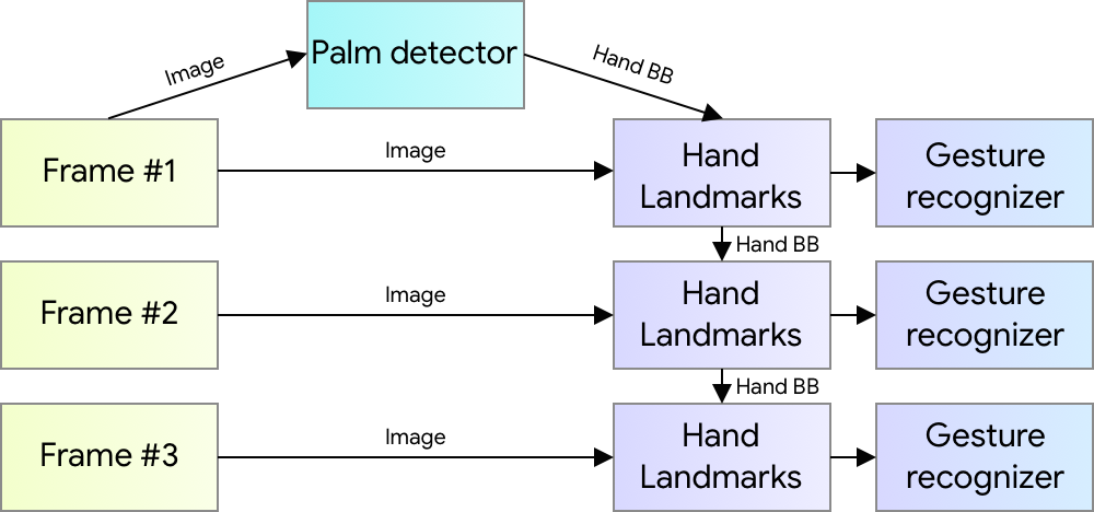
Object detection is an extensively studied computer vision problem, but most of the research has focused on 2D object prediction. While 2D prediction only provides 2D bounding boxes, by extending prediction to 3D, one can capture an object’s size, position and orientation in the world, leading to a variety of applications in robotics, self-driving vehicles, image retrieval, and augmented reality. Although 2D object detection is relatively mature and has been widely used in the industry, 3D object detection from 2D imagery is a challenging problem, due to the lack of data and diversity of appearances and shapes of objects within a category.

Today, we are announcing the release of MediaPipe Objectron, a mobile real-time 3D object detection pipeline for everyday objects. This pipeline detects objects in 2D images, and estimates their poses and sizes through a machine learning (ML) model, trained on a newly created 3D dataset. Implemented in MediaPipe, an open-source cross-platform framework for building pipelines to process perceptual data of different modalities, Objectron computes oriented 3D bounding boxes of objects in real-time on mobile devices.
 
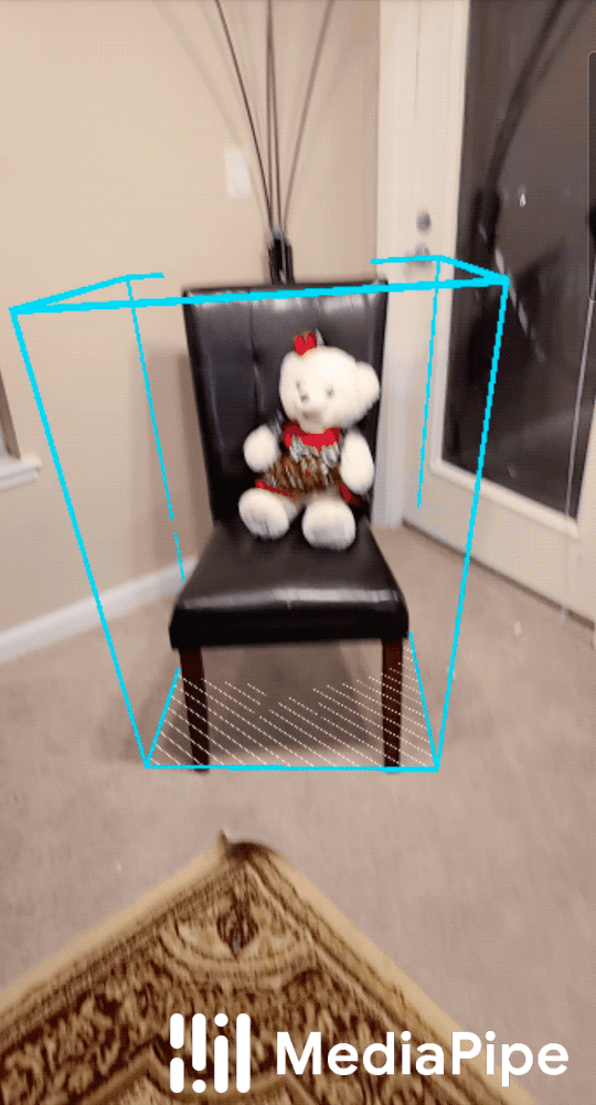
3D Object Detection from a single image. MediaPipe Objectron determines the position, orientation and size of everyday objects in real-time on mobile devices.
Obtaining Real-World 3D Training Data
While there are ample amounts of 3D data for street scenes, due to the popularity of research into self-driving cars that rely on 3D capture sensors like LIDAR, datasets with ground truth 3D annotations for more granular everyday objects are extremely limited. To overcome this problem, we developed a novel data pipeline using mobile augmented reality (AR) session data. With the arrival of ARCore and ARKit, hundreds of millions of smartphones now have AR capabilities and the ability to capture additional information during an AR session, including the camera pose, sparse 3D point clouds, estimated lighting, and planar surfaces.

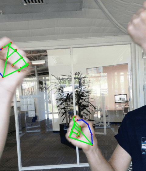
In order to label ground truth data, we built a novel annotation tool for use with AR session data, which allows annotators to quickly label 3D bounding boxes for objects. This tool uses a split-screen view to display 2D video frames on which are overlaid 3D bounding boxes on the left, alongside a view showing 3D point clouds, camera positions and detected planes on the right. Annotators draw 3D bounding boxes in the 3D view, and verify its location by reviewing the projections in 2D video frames. For static objects, we only need to annotate an object in a single frame and propagate its location to all frames using the ground truth camera pose information from the AR session data, which makes the procedure highly efficient.
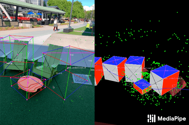
Real-world data annotation for 3D object detection. Right: 3D bounding boxes are annotated in the 3D world with detected surfaces and point clouds. Left: Projections of annotated 3D bounding boxes are overlaid on top of video frames making it easy to validate the annotation.
AR Synthetic Data Generation
A popular approach is to complement real-world data with synthetic data in order to increase the accuracy of prediction. However, attempts to do so often yield poor, unrealistic data or, in the case of photorealistic rendering, require significant effort and compute. Our novel approach, called AR Synthetic Data Generation, places virtual objects into scenes that have AR session data, which allows us to leverage camera poses, detected planar surfaces, and estimated lighting to generate placements that are physically probable and with lighting that matches the scene. This approach results in high-quality synthetic data with rendered objects that respect the scene geometry and fit seamlessly into real backgrounds. By combining real-world data and AR synthetic data, we are able to increase the accuracy by about 10%.
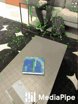
An example of AR synthetic data generation. The virtual white-brown cereal box is rendered into the real scene, next to the real blue book.
An ML Pipeline for 3D Object Detection
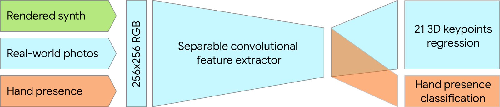
We built a single-stage model to predict the pose and physical size of an object from a single RGB image. The model backbone has an encoder-decoder architecture, built upon MobileNetv2. We employ a multi-task learning approach, jointly predicting an object's shape with detection and regression. The shape task predicts the object's shape signals depending on what ground truth annotation is available, e.g. segmentation. This is optional if there is no shape annotation in training data. For the detection task, we use the annotated bounding boxes and fit a Gaussian to the box, with center at the box centroid, and standard deviations proportional to the box size. The goal for detection is then to predict this distribution with its peak representing the object’s center location. The regression task estimates the 2D projections of the eight bounding box vertices. To obtain the final 3D coordinates for the bounding box, we leverage a well established pose estimation algorithm (EPnP). It can recover the 3D bounding box of an object, without a priori knowledge of the object dimensions. Given the 3D bounding box, we can easily compute pose and size of the object. The diagram below shows our network architecture and post-processing. The model is light enough to run real-time on mobile devices (at 26 FPS on an Adreno 650 mobile GPU).
Network architecture and post-processing for 3D object detection.
Sample results of our network — [left] original 2D image with estimated bounding boxes, [middle] object detection by Gaussian distribution, [right] predicted segmentation mask.
Detection and Tracking in MediaPipe
When the model is applied to every frame captured by the mobile device, it can suffer from jitter due to the ambiguity of the 3D bounding box estimated in each frame. To mitigate this, we adopt the detection+tracking framework recently released in our 2D object detection and tracking solution. This framework mitigates the need to run the network on every frame, allowing the use of heavier and therefore more accurate models, while keeping the pipeline real-time on mobile devices. It also retains object identity across frames and ensures that the prediction is temporally consistent, reducing the jitter.

For further efficiency in our mobile pipeline, we run our model inference only once every few frames. Next, we take the prediction and track it over time using the approach described in our previous blogs for instant motion tracking and Motion Stills. When a new prediction is made, we consolidate the detection result with the tracking result based on the area of overlap.

To encourage researchers and developers to experiment and prototype based on our pipeline, we are releasing our on-device ML pipeline in MediaPipe, including an end-to-end demo mobile application and our trained models for two categories: shoes and chairs. We hope that sharing our solution with the wide research and development community will stimulate new use cases, new applications, and new research efforts. In the future, we plan to scale our model to many more categories, and further improve our on-device performance.
   
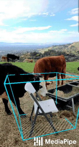
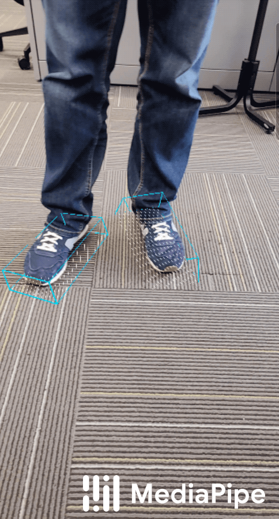
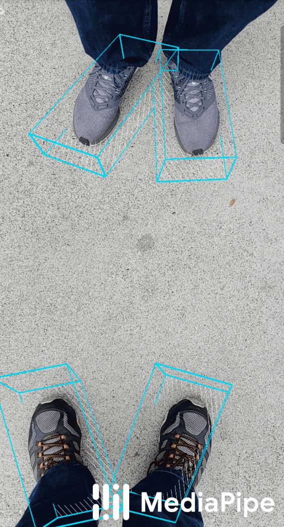
Examples of our 3D object detection in the wild.
Acknowledgements
The research described in this post was done by Adel Ahmadyan, Tingbo Hou, Jianing Wei, Matthias Grundmann, Liangkai Zhang, Jiuqiang Tang, Chris McClanahan, Tyler Mullen, Buck Bourdon, Esha Uboweja, Mogan Shieh, Siarhei Kazakou, Ming Guang Yong, Chuo-Ling Chang, and James Bruce. We thank Aliaksandr Shyrokau and the annotation team for their diligence to high quality annotations.

Source: Google AI Blog


Enhancing the Research Community’s Access to Street View Panoramas for Language Grounding Tasks


Significant advances continue to be made in both natural language processing and computer vision, but the research community is still far from having computer agents that can interpret instructions in a real-world visual context and take appropriate actions based on those instructions. Agents, including robots, can learn to navigate new environments, but they cannot yet understand instructions such as, “Go forward and turn left after the red fire hydrant by the train tracks. Then go three blocks and stop in front of the building with a row of flags over its entrance.” Doing so requires relating verbal descriptions like train tracks, red fire hydrant, and row of flags to their visual appearance, understanding what a block is and how to count three of them, relating objects based on spatial configurations such as by and over, relating directions such as go forward and turn left to actions, and much more.

Grounded language understanding problems of this form are excellent testbeds for research on computational intelligence in that they are easy for people but hard for current agents, they synthesize language, perception and action, and evaluation of successful completion is straightforward. Progress on such problems can greatly enhance the ability of agents to coordinate movement and action with people. However finding or creating datasets large and diverse enough for developing robust models is difficult.

An ideal resource for quickly training and evaluating agents on grounded language understanding tasks is Street View imagery, an extensive and visually rich virtual representation of the world. Street View is integrated with Google Maps and is composed of billions of street-level panoramas. The Touchdown dataset, created by researchers at Cornell Tech, represents a compelling example of using Street View to drive research on grounded language understanding. However, due to restrictions on access to Street View panoramas, Touchdown can only provide panorama IDs rather than the panoramas themselves, sometimes making it difficult for the broader research community to work on Touchdown’s tasks: vision-and-language navigation (VLN), in which instructions are presented for navigation through streets, and spatial description resolution (SDR), which requires resolving spatial descriptions from a given viewpoint.

In “Retouchdown: Adding Touchdown to StreetLearn as a Shareable Resource for Language Grounding Tasks in Street View,” we address this problem by adding the Street View panoramas referenced in the Touchdown tasks to the existing StreetLearn dataset. Using this data, we generate a model that is fully compatible with the tasks defined in Touchdown. Additionally, we have provided open source TensorFlow implementations for the Touchdown tasks as part of the VALAN toolkit.

Grounded Language Understanding Tasks
Touchdown’s two grounded language understanding tasks can be used as benchmarks for navigation models. VLN involves following instructions from one street location to another, while SDR requires identifying a point in a Street View panorama given a description based on its surrounding visual context. The two tasks are shown being performed together in the animation below.
Example animation of a person following Touchdown instructions: “Orient yourself so that the umbrellas are to the right. Go straight and take a right at the first intersection. At the next intersection there should be an old-fashioned store to the left. There is also a dinosaur mural to the right. Touchdown is on the back of the dinosaur.”
Touchdown’s VLN task is similar to that defined in the popular Room-to-Room dataset, except that Street View has far greater visual diversity and more degrees of freedom for movement. Performance of the baseline models in Touchdown leaves considerable headroom for innovation and improvement on many facets of the task, including linguistic and visual representations, their integration, and learning to take actions conditioned on them.

That said, while enabling the broader research community to work with Touchdown’s tasks, certain safeguards are needed to make it compliant with the Google Maps/Google Earth Terms of Service and protect the needs of both Google and individuals. For example, panoramas may not be mass downloaded, nor can they be stored indefinitely (for example, individuals may ask to remove specific panoramas). Therefore, researchers must periodically delete and refresh panoramas in order to work with the data while remaining compliant with these terms.

StreetLearn: A Dataset of Approved Panoramas for Research Use
An alternative way to interact with Street View panoramas was forged by DeepMind with the StreetLearn data release last year. With StreetLearn, interested researchers can fill out a form requesting access to a set of 114k panoramas for regions of New York City and Pittsburgh. Recently, StreetLearn has been used to support the StreetNav task suite, which includes training and evaluating agents that follow Google Maps directions. This is a VLN task like Touchdown and Room-to-Room; however, it differs greatly in that it does not use natural language provided by people.

Additionally, even though StreetLearn’s panoramas cover the same area of Manhattan as Touchdown, they are not adequate for research covering the tasks defined in Touchdown, because those tasks require the exact panoramas that were used during the Touchdown annotation process. For example, in Touchdown tasks, the language instructions refer to transient objects such as cars, bicycles, and couches. A Street View panorama from a different time period may not contain these objects, so the instructions are not stable across time periods.
Touchdown instruction: “Two parked bicycles, and a discarded couch, all on the left. Walk just past this couch, and stop before you pass another parked bicycle. This bike will be white and red, with a white seat. Touchdown is sitting on top of the bike seat.” Other panoramas from the same location taken at other times would be highly unlikely to contain these exact items in the exact same positions. For a concrete example, see the current imagery available for this location in Street View, which contains very different transient objects.
Furthermore, SDR requires coverage of multiple points-of-view for those specific panoramas. For example, the following panorama is one step down the street from the previous one. They may look similar, but they are in fact quite different — note that the bikes seen on the left side in both panoramas are not  the same — and the location of Touchdown is toward the middle of the above panorama (on the bike seat) and to the bottom left in the second panorama. As such, the pixel location of the SDR problem is different for different panoramas, but consistent with respect to the real world location referred to in the instruction. This is especially important for the end-to-end task of following both the VLN and SDR instructions together: if an agent stops, they should be able to complete the SDR task regardless of their exact location (provided the target is visible).
A panorama one step farther down the street from the previous scene.
Another problem is that the granularity of the panorama spacing is different. The figure below shows the overlap between the StreetLearn (blue) and Touchdown (red) panoramas in Manhattan. There are 710 panoramas (out of 29,641) that share the same ID in both datasets (in black). Touchdown covers half of Manhattan and the density of the panoramas is similar, but the exact locations of the nodes visited differ.
Adding Touchdown Panoramas to StreetLearn and Verifying Model Baselines
Retouchdown reconciles Touchdown’s mode of dissemination with StreetLearn’s, which was originally designed to adhere to the rights of Google and individuals while also simplifying access to researchers and improving reproducibility. Retouchdown includes both data and code that allows the broader research community to work effectively with the Touchdown tasks — most importantly to ensure access to the data and to ease reproducibility. To this end, we have integrated the Touchdown panoramas into the StreetLearn dataset to create a new version of StreetLearn with 144k panoramas (an increase of 26%) that are all approved for research use.

We also reimplemented models for VLN and SDR and show that they are on par or better than the results obtained in the original Touchdown paper. These implementations are open-sourced as well, as part of the VALAN toolkit. The first graph below compares the results of Chen et al. (2019) to our reimplementation for the VLN task. It includes the SDTW metric, which measures both successful completion and fidelity to the true reference path. The second graph below makes the same comparison for the SDR task. For SDR, we show accuracy@npx measurements, which provides the percent of times the model’s prediction is within n pixels of the goal location in the image. Our results are slightly better due to some small differences in models and processing, but most importantly, the results show that the updated panoramas are fully capable of supporting future modeling for the Touchdown tasks.
Performance comparison between Chen et al. (2019) using the original panoramas (in blue) and our reimplementation using the panoramas available in StreetLearn (in red). Top: VLN results for task completion, shortest path distance and success weighted by Dynamic Time Warping (SDTW). Bottom: SDR results for the accuracy@npx metrics.
Obtaining the Data
Researchers interested in working with the panoramas should fill out the StreetLearn interest form. Subject to approval, they will be provided with a download link. Their information is held so that the StreetLearn team can inform them of updates to the data. This allows both Google and participating researchers to effectively and easily respect takedown requests. The instructions and panorama connectivity data can be obtained from the Touchdown github repository.

It is our hope that this release of these additional panoramas will enable the research community to make further progress on these challenging grounded language understanding tasks.

Acknowledgements
The core team includes Yoav Artzi, Eugene Ie, and Piotr Mirowski. We would like to thank Howard Chen for his help with reproducing the Touchdown results, Larry Lansing, Valts Blukis and Vihan Jain for their help with the code and open-sourcing, and the Language team in Google Research, especially Radu Soricut, for the insightful comments that contributed to this work. Many thanks also to the Google Maps and Google Street View teams for their support in accessing and releasing the data, and to the Data Compute team for reviewing the panoramas.

Source: Google AI Blog


Announcing the Third Workshop and Challenge on Learned Image Compression


With the large amount of media content being downloaded and streamed across the internet, minimizing bandwidth while maintaining quality remains a constant challenge. In 2015, researchers demonstrated that neural network-based image compression could yield significant improvements to image resolution while retaining good quality and high compression speed. Continued advances in compression and bandwidth optimization techniques were stimulated in part by two successful workshops that we hosted at CVPR in 2018 and 2019.

Today, we are excited to announce the Third Workshop and Challenge On Learned Image Compression (CLIC) at CVPR 2020. This workshop challenges researchers to use machine learning, neural networks and other computer vision approaches to increase the quality and lower the bandwidth needed for multimedia transmission. This year’s workshop will also include two challenges: a low-rate image compression challenge and a P-Frame video compression challenge.

Similar to previous years, the goal of the low-rate image compression challenge is to compress an image dataset to 0.15 bits per pixel while maintaining the highest possible quality. Finalists will be selected by measuring their performance against the PSNR and MS-SSIM evaluation metrics. The final ranking will then be determined by a human evaluated rating task.

This year we are also introducing a P-Frame compression track, the first video compression task in this series. In this challenge, participants must first generate a transformation between two adjacent video frames. In the decompression part of the task, participants then use the first frame and their compressed representation to reconstruct the second frame. This challenge will be ranked based solely on the MS-SSIM performance score.

If you are doing research in the field of learned image compression or video compression, we encourage you to participate in CLIC, whether in the two competitions or the paper-only track for publications to be presented at the workshop at CVPR 2020. The validation server is currently available for submissions. The deadline for the final submission of the test set is March 23rd, 2020. For more details on the competition and an up-to-date schedule, please refer to compression.cc. Additional announcements and answers to questions can be found on our Google Groups page.

Acknowledgements
This workshop is being jointly hosted by researchers at Google, Twitter and ETH Zurich. We’d like to thank: George Toderici (Google), Nick Johnston (Google), Johannes Ballé (Google), Eirikur Agustsson (Google), Lucas Theis (Google), Wenzhe Shi (Twitter), Radu Timofte (ETH Zurich) and Fabian Mentzer (ETH Zurich) for their contributions.

Source: Google AI Blog


Developing Deep Learning Models for Chest X-rays with Adjudicated Image Labels


With millions of diagnostic examinations performed annually, chest X-rays are an important and accessible clinical imaging tool for the detection of many diseases. However, their usefulness can be limited by challenges in interpretation, which requires rapid and thorough evaluation of a two-dimensional image depicting complex, three-dimensional organs and disease processes. Indeed, early-stage lung cancers or pneumothoraces (collapsed lungs) can be missed on chest X-rays, leading to serious adverse outcomes for patients.

Advances in machine learning (ML) present an exciting opportunity to create new tools to help experts interpret medical images. Recent efforts have shown promise in improving lung cancer detection in radiology, prostate cancer grading in pathology, and differential diagnoses in dermatology. For chest X-ray images in particular, large, de-identified public image sets are available to researchers across disciplines, and have facilitated several valuable efforts to develop deep learning models for X-ray interpretation. However, obtaining accurate clinical labels for the very large image sets needed for deep learning can be difficult. Most efforts have either applied rule-based natural language processing (NLP) to radiology reports or relied on image review by individual readers, both of which may introduce inconsistencies or errors that can be especially problematic during model evaluation. Another challenge involves assembling datasets that represent an adequately diverse spectrum of cases (i.e., ensuring inclusion of both “hard” cases and “easy” cases that represent the full spectrum of disease presentation). Finally, some chest X-ray findings are non-specific and depend on clinical information about the patient to fully understand their significance. As such, establishing labels that are clinically meaningful and have consistent definitions can be a challenging component of developing machine learning models that use only the image as input. Without standardized and clinically meaningful datasets as well as rigorous reference standard methods, successful application of ML to interpretation of chest X-rays will be hindered.

To help address these issues, we recently published “Chest Radiograph Interpretation with Deep Learning Models: Assessment with Radiologist-adjudicated Reference Standards and Population-adjusted Evaluation” in the journal Radiology. In this study we developed deep learning models to classify four clinically important findings on chest X-rays — pneumothorax, nodules and masses, fractures, and airspace opacities. These target findings were selected in consultation with radiologists and clinical colleagues, so as to focus on conditions that are both critical for patient care and for which chest X-ray images alone are an important and accessible first-line imaging study. Selection of these findings also allowed model evaluation using only de-identified images without additional clinical data.

Models were evaluated using thousands of held-out images from each dataset for which we collected high-quality labels using a panel-based adjudication process among board-certified radiologists. Four separate radiologists also independently reviewed the held-out images in order to compare radiologist accuracy to that of the deep learning models (using the panel-based image labels as the reference standard). For all four findings and across both datasets, the deep learning models demonstrated radiologist-level performance. We are sharing the adjudicated labels for the publicly available data here to facilitate additional research.

Data Overview
This work leveraged over 600,000 images sourced from two de-identified datasets. The first dataset was developed in collaboration with co-authors at the Apollo Hospitals, and consists of a diverse set of chest X-rays obtained over several years from multiple locations across the Apollo Hospitals network. The second dataset is the publicly available ChestX-ray14 image set released by the National Institutes of Health (NIH). This second dataset has served as an important resource for many machine learning efforts, yet has limitations stemming from issues with the accuracy and clinical interpretation of the currently available labels.
Chest X-ray depicting an upper left lobe pneumothorax identified by the model and the adjudication panel, but missed by the individual radiologist readers. Left: The original image. Right: The same image with the most important regions for the model prediction highlighted in orange.
Training Set Labels Using Deep Learning and Visual Image Review
For very large datasets consisting of hundreds of thousands of images, such as those needed to train highly accurate deep learning models, it is impractical to manually assign image labels. As such, we developed a separate, text-based deep learning model to extract image labels using the de-identified radiology reports associated with each X-ray. This NLP model was then applied to provide labels for over 560,000 images from the Apollo Hospitals dataset used for training the computer vision models.

To reduce noise from any errors introduced by the text-based label extraction and also to provide the relevant labels for a substantial number of the ChestX-ray14 images, approximately 37,000 images across the two datasets were visually reviewed by radiologists. These were separate from the NLP-based labels and helped to ensure high quality labels across such a large, diverse set of training images.

Creating and Sharing Improved Reference Standard Labels
To generate high-quality reference standard labels for model evaluation, we utilized a panel-based adjudication process, whereby three radiologists reviewed all final tune and test set images and resolved disagreements through discussion. This often allowed difficult findings that were initially only detected by a single radiologist to be identified and documented appropriately. To reduce the risk of bias based on any individual radiologist’s personality or seniority, the discussions took place anonymously via an online discussion and adjudication system.

Because the lack of available adjudicated labels was a significant initial barrier to our work, we are sharing with the research community all of the adjudicated labels for the publicly available ChestX-ray14 dataset, including 2,412 training/validation set images and 1,962 test set images (4,374 images in total). We hope that these labels will facilitate future machine learning efforts and enable better apples-to-apples comparisons between machine learning models for chest X-ray interpretation.

Future Outlook
This work presents several contributions: (1) releasing adjudicated labels for images from a publicly available dataset; (2) a method to scale accurate labeling of training data using a text-based deep learning model; (3) evaluation using a diverse set of images with expert-adjudicated reference standard labels; and ultimately (4) radiologist-level performance of deep learning models for clinically important findings on chest X-rays.

However, in regards to model performance, achieving expert-level accuracy on average is just a part of the story. Even though overall accuracy for the deep learning models was consistently similar to that of radiologists for any given finding, performance for both varied across datasets. For example, the sensitivity for detecting pneumothorax among radiologists was approximately 79% for the ChestX-ray14 images, but was only 52% for the same radiologists on the other dataset, suggesting a more difficult collection cases in the latter. This highlights the importance of validating deep learning tools on multiple, diverse datasets and eventually across the patient populations and clinical settings in which any model is intended to be used.

The performance differences between datasets also emphasize the need for standardized evaluation image sets with accurate reference standards in order to allow comparison across studies. For example, if two different models for the same finding were evaluated using different datasets, comparing performance would be of minimal value without knowing additional details such as the case mix, model error modes, or radiologist performance on the same cases.

Finally, the model often identified findings that were consistently missed by radiologists, and vice versa. As such, strategies that combine the unique “skills” of both the deep learning systems and human experts are likely to hold the most promise for realizing the potential of AI applications in medical image interpretation.

Acknowledgements
Key contributors to this project at Google include Sid Mittal, Gavin Duggan, Anna Majkowska, Scott McKinney, Andrew Sellergren, David Steiner, Krish Eswaran, Po-Hsuan Cameron Chen, Yun Liu, Shravya Shetty, and Daniel Tse. Significant contributions and input were also made by radiologist collaborators Joshua Reicher, Alexander Ding, and Sreenivasa Raju Kalidindi. The authors would also like to acknowledge many members of the Google Health radiology team including Jonny Wong, Diego Ardila, Zvika Ben-Haim, Rory Sayres, Shahar Jamshy, Shabir Adeel, Mikhail Fomitchev, Akinori Mitani, Quang Duong, William Chen and Sahar Kazemzadeh. Sincere appreciation also goes to the many radiologists who enabled this work through their expert image interpretation efforts throughout the project.

Source: Google AI Blog


Project Ihmehimmeli: Temporal Coding in Spiking Neural Networks


The discoveries being made regularly in neuroscience are an ongoing source of inspiration for creating more efficient artificial neural networks that process information in the same way as biological organisms. These networks have recently achieved resounding success in domains ranging from playing board and video games to fine-grained understanding of video. However, there is one fundamental aspect of biological brains that artificial neural networks are not yet fully leveraging: temporal encoding of information. Preserving temporal information allows a better representation of dynamic features, such as sounds, and enables fast responses to events that may occur at any moment. Furthermore, despite the fact that biological systems can consist of billions of neurons, information can be carried by a single signal (‘spike’) fired by an individual neuron, with information encoded in the timing of the signal itself.

Based on this biological insight, project Ihmehimmeli explores how artificial spiking neural networks can exploit temporal dynamics using various architectures and learning settings. “Ihmehimmeli” is a Finnish tongue-in-cheek word for a complex tool or a machine element whose purpose is not immediately easy to grasp. The essence of this word captures our aim to build complex recurrent neural network architectures with temporal encoding of information. We use artificial spiking networks with a temporal coding scheme, in which more interesting or surprising information, such as louder sounds or brighter colours, causes earlier neuronal spikes. Along the information processing hierarchy, the winning neurons are those that spike first. Such an encoding can naturally implement a classification scheme where input features are encoded in the spike times of their corresponding input neurons, while the output class is encoded by the output neuron that spikes earliest.
The Ihmehimmeli project team holding a himmeli, a symbol for the aim to build recurrent neural network architectures with temporal encoding of information.
We recently published and open-sourced a model in which we demonstrated the computational capabilities of fully connected spiking networks that operate using temporal coding. Our model uses a biologically-inspired synaptic transfer function, where the electric potential on the membrane of a neuron rises and gradually decays over time in response to an incoming signal, until there is a spike. The strength of the associated change is controlled by the "weight" of the connection, which represents the synapse efficiency. Crucially, this formulation allows exact derivatives of postsynaptic spike times with respect to presynaptic spike times and weights. The process of training the network consists of adjusting the weights between neurons, which in turn leads to adjusted spike times across the network. Much like in conventional artificial neural networks, this was done using backpropagation. We used synchronization pulses, whose timing is also learned with backpropagation, to provide a temporal reference to the network.

We trained the network on classic machine learning benchmarks, with features encoded in time. The spiking network successfully learned to solve noisy Boolean logic problems and achieved a test accuracy of 97.96% on MNIST, a result comparable to conventional fully connected networks with the same architecture. However, unlike conventional networks, our spiking network uses an encoding that is in general more biologically-plausible, and, for a small trade-off in accuracy, can compute the result in a highly energy-efficient manner, as detailed below.

While training the spiking network on MNIST, we observed the neural network spontaneously shift between two operating regimes. Early during training, the network exhibited a slow and highly accurate regime, where almost all neurons fired before the network made a decision. Later in training, the network spontaneously shifted into a fast but slightly less accurate regime. This behaviour was intriguing, as we did not optimize for it explicitly. Thus spiking networks can, in a sense, be “deliberative”, or make a snap decision on the spot. This is reminiscent of the trade-off between speed and accuracy in human decision-making.
A slow (“deliberative”) network (top) and a fast (“impulsive”) network (bottom) classifying the same MNIST digit. The figures show a raster plot of spike times of individual neurons in individual layers, with synchronization pulses shown in orange. In this example, both networks classify the digit correctly; overall, the “slow” network achieves better accuracy than the “fast” network.
We were also able to recover representations of the digits learned by the spiking network by gradually adjusting a blank input image to maximize the response of a target output neuron. This indicates that the network learns human-like representations of the digits, as opposed to other possible combinations of pixels that might look “alien” to people. Having interpretable representations is important in order to understand what the network is truly learning and to prevent a small change in input from causing a large change in the result.
How the network “imagines” the digits 0, 1, 3 and 7.
This work is one example of an initial step that project Ihmehimmeli is taking in exploring the potential of time-based biology-inspired computing. In other on-going experiments, we are training spiking networks with temporal coding to control the walking of an artificial insect in a virtual environment, or taking inspiration from the development of the neural system to train a 2D spiking grid to predict words using axonal growth. Our goal is to increase our familiarity with the mechanisms that nature has evolved for natural intelligence, enabling the exploration of time-based artificial neural networks with varying internal states and state transitions.

Acknowledgements
The work described here was authored by Iulia Comsa, Krzysztof Potempa, Luca Versari, Thomas Fischbacher, Andrea Gesmundo and Jyrki Alakuijala. We are grateful for all discussions and feedback on this work that we received from our colleagues at Google.

Source: Google AI Blog


Learning Cross-Modal Temporal Representations from Unlabeled Videos


While people can easily recognize what activities are taking place in videos and anticipate what events may happen next, it is much more difficult for machines. Yet, increasingly, it is important for machines to understand the contents and dynamics of videos for applications, such as temporal localization, action detection and navigation for self-driving cars. In order to train neural networks to perform such tasks, it is common to use supervised training, in which the training data consists of videos that have been meticulously labeled by people on a frame-by-frame basis. Such annotations are hard to acquire at scale. Consequently, there is much interest in self-supervised learning, in which models are trained on various proxy tasks, and the supervision of those tasks naturally resides in the data itself.

In “VideoBERT: A Joint Model for Video and Language Representation Learning” (VideoBERT) and “Contrastive Bidirectional Transformer for Temporal Representation Learning” (CBT), we propose to learn temporal representations from unlabeled videos. The goal is to discover high-level semantic features that correspond to actions and events that unfold over longer time scales. To accomplish this, we exploit the key insight that human language has evolved words to describe high-level objects and events. In videos, speech tends to be temporally aligned with the visual signals, and can be extracted by using off-the-shelf automatic speech recognition (ASR) systems, and thus provides a natural source of self-supervision. Our model is an example of cross-modal learning, as it jointly utilizes the signals from visual and audio (speech) modalities during training.
Image frames and human speech from the same video locations are often semantically aligned. The alignment is non-exhaustive and sometimes noisy, which we hope to mitigate by pretraining on larger datasets. For the left example, the ASR output is, “Keep rolling tight and squeeze the air out to its side and you can kind of pull a little bit.”, where the actions are captured by speech but the objects are not. For the right example, the ASR output is, “This is where you need to be patient patient patient,” which is not related to the visual content at all.
A BERT Model for Videos
The first step of representation learning is to define a proxy task that leads the model to learn temporal dynamics and cross-modal semantic correspondence from long, unlabeled videos. To this end, we generalize the Bidirectional Encoder Representations from Transformers (BERT) model. The BERT model has shown state-of-the-art performance on various natural language processing tasks, by applying the Transformer architecture to encode long sequences, and pretraining on a corpus containing a large amount of text. BERT uses the cloze test as its proxy task, in which the BERT model is forced to predict missing words from context bidirectionally, instead of just predicting the next word in a sequence.

To do this, we generalize the BERT training objective, using image frames combined with the ASR sentence output at the same locations to compose cross-modal “sentences”. The image frames are converted into visual tokens with durations of 1.5 seconds, based on visual feature similarities. They are then concatenated with the ASR word tokens. We train the VideoBERT model to fill out the missing tokens from the visual-text sentences. Our hypothesis, which our experiments support, is that by pretraining on this proxy task, the model learns to reason about longer-range temporal dynamics (visual cloze) and high-level semantics (visual-text cloze).
Illustration of VideoBERT in the context of a video and text masked token prediction, or cloze, task. Bottom: visual and text (ASR) tokens from the same locations of videos are concatenated to form the inputs to VideoBERT. Some visual and text tokens are masked out. Middle: VideoBERT applies the Transformer architecture to jointly encode bidirectional visual-text context. Yellow and pink boxes correspond to the input and output embeddings, respectively. Top: the training objective is to recover the correct tokens for the masked locations.
Inspecting the VideoBERT Model
We trained VideoBERT on over one million instructional videos, such as cooking, gardening and vehicle repair. Once trained, one can inspect what the VideoBERT model learns on a number of tasks to verify that the output accurately reflects the video content. For example, text-to-video prediction can be used to automatically generate a set of instructions (such as a recipe) from video, yielding video segments (tokens) that reflect what is described at each step. In addition, video-to-video prediction can be used to visualize possible future content based on an initial video token.
Qualitative results from VideoBERT, pretrained on cooking videos. Top: Given some recipe text, we generate a sequence of visual tokens. Bottom: Given a visual token, we show the top three future tokens forecast by VideoBERT at different time scales. In this case, the model predicts that a bowl of flour and cocoa powder may be baked in an oven, and may become a brownie or cupcake. We visualize the visual tokens using the images from the training set closest to the tokens in feature space.
To verify if VideoBERT learns semantic correspondences between videos and text, we tested its “zero-shot” classification accuracy on a cooking video dataset in which neither the videos nor annotations were used during pre-training. To perform classification, the video tokens were concatenated with a template sentence “now let me show you how to [MASK] the [MASK]” and the predicted verb and noun tokens were extracted. The VideoBERT model matched the top-5 accuracy of a fully-supervised baseline, indicating that the model is able to perform competitively in this “zero-shot” setting.

Transfer Learning with Contrastive Bidirectional Transformers
While VideoBERT showed impressive results in learning how to automatically label and predict video content, we noticed that the visual tokens used by VideoBERT can lose fine-grained visual information, such as smaller objects and subtle motions. To explore this, we propose the Contrastive Bidirectional Transformers (CBT) model which removes this tokenization step, and further evaluated the quality of learned representations by transfer learning on downstream tasks. CBT applies a different loss function, the contrastive loss, in order to maximize the mutual information between the masked positions and the rest of cross-modal sentences. We evaluated the learned representations for a diverse set of tasks (e.g., action segmentation, action anticipation and video captioning) and on various video datasets. The CBT approach outperforms previous state-of-the-art by significant margins on most benchmarks. We observe that: (1) the cross-modal objective is important for transfer learning performance; (2) a bigger and more diverse pre-training set leads to better representations; (3) compared with baseline methods such as average pooling or LSTMs, the CBT model is much better at utilizing long temporal context.
Action anticipation accuracy with the CBT approach from untrimmed videos with 200 activity classes. We compare with AvgPool and LSTM, and report performance when the observation time is 15, 30, 45 and 72 seconds.
Conclusion & future work
Our results demonstrate the power of the BERT model for learning visual-linguistic and visual representations from unlabeled videos. We find that our models are not only useful for zero-shot action classification and recipe generation, but the learned temporal representations also transfer well to various downstream tasks, such as action anticipation. Future work includes learning low-level visual features jointly with long-term temporal representations, which enables better adaptation to the video context. Furthermore, we plan to expand the number of pre-training videos to be larger and more diverse.

Acknowledgements
The core team includes Chen Sun, Fabien Baradel, Austin Myers, Carl Vondrick, Kevin Murphy and Cordelia Schmid. We would like to thank Jack Hessel, Bo Pang, Radu Soricut, Baris Sumengen, Zhenhai Zhu, and the BERT team for sharing amazing tools that greatly facilitated our experiments. We also thank Justin Gilmer, Abhishek Kumar, Ben Poole, David Ross, and Rahul Sukthankar for helpful discussions.

Source: Google AI Blog


On-Device, Real-Time Hand Tracking with MediaPipe


The ability to perceive the shape and motion of hands can be a vital component in improving the user experience across a variety of technological domains and platforms. For example, it can form the basis for sign language understanding and hand gesture control, and can also enable the overlay of digital content and information on top of the physical world in augmented reality. While coming naturally to people, robust real-time hand perception is a decidedly challenging computer vision task, as hands often occlude themselves or each other (e.g. finger/palm occlusions and hand shakes) and lack high contrast patterns.

Today we are announcing the release of a new approach to hand perception, which we previewed CVPR 2019 in June, implemented in MediaPipe—an open source cross platform framework for building pipelines to process perceptual data of different modalities, such as video and audio. This approach provides high-fidelity hand and finger tracking by employing machine learning (ML) to infer 21 3D keypoints of a hand from just a single frame. Whereas current state-of-the-art approaches rely primarily on powerful desktop environments for inference, our method achieves real-time performance on a mobile phone, and even scales to multiple hands. We hope that providing this hand perception functionality to the wider research and development community will result in an emergence of creative use cases, stimulating new applications and new research avenues.
3D hand perception in real-time on a mobile phone via MediaPipe. Our solution uses machine learning to compute 21 3D keypoints of a hand from a video frame. Depth is indicated in grayscale.
An ML Pipeline for Hand Tracking and Gesture Recognition
Our hand tracking solution utilizes an ML pipeline consisting of several models working together:
  • A palm detector model (called BlazePalm) that operates on the full image and returns an oriented hand bounding box.
  • A hand landmark model that operates on the cropped image region defined by the palm detector and returns high fidelity 3D hand keypoints.
  • A gesture recognizer that classifies the previously computed keypoint configuration into a discrete set of gestures.
This architecture is similar to that employed by our recently published face mesh ML pipeline and that others have used for pose estimation. Providing the accurately cropped palm image to the hand landmark model drastically reduces the need for data augmentation (e.g. rotations, translation and scale) and instead allows the network to dedicate most of its capacity towards coordinate prediction accuracy.
Hand perception pipeline overview.
BlazePalm: Realtime Hand/Palm Detection
To detect initial hand locations, we employ a single-shot detector model called BlazePalm, optimized for mobile real-time uses in a manner similar to BlazeFace, which is also available in MediaPipe. Detecting hands is a decidedly complex task: our model has to work across a variety of hand sizes with a large scale span (~20x) relative to the image frame and be able to detect occluded and self-occluded hands. Whereas faces have high contrast patterns, e.g., in the eye and mouth region, the lack of such features in hands makes it comparatively difficult to detect them reliably from their visual features alone. Instead, providing additional context, like arm, body, or person features, aids accurate hand localization.

Our solution addresses the above challenges using different strategies. First, we train a palm detector instead of a hand detector, since estimating bounding boxes of rigid objects like palms and fists is significantly simpler than detecting hands with articulated fingers. In addition, as palms are smaller objects, the non-maximum suppression algorithm works well even for two-hand self-occlusion cases, like handshakes. Moreover, palms can be modelled using square bounding boxes (anchors in ML terminology) ignoring other aspect ratios, and therefore reducing the number of anchors by a factor of 3-5. Second, an encoder-decoder feature extractor is used for bigger scene context awareness even for small objects (similar to the RetinaNet approach). Lastly, we minimize the focal loss during training to support a large amount of anchors resulting from the high scale variance.

With the above techniques, we achieve an average precision of 95.7% in palm detection. Using a regular cross entropy loss and no decoder gives a baseline of just 86.22%.

Hand Landmark Model
After the palm detection over the whole image our subsequent hand landmark model performs precise keypoint localization of 21 3D hand-knuckle coordinates inside the detected hand regions via regression, that is direct coordinate prediction. The model learns a consistent internal hand pose representation and is robust even to partially visible hands and self-occlusions.

To obtain ground truth data, we have manually annotated ~30K real-world images with 21 3D coordinates, as shown below (we take Z-value from image depth map, if it exists per corresponding coordinate). To better cover the possible hand poses and provide additional supervision on the nature of hand geometry, we also render a high-quality synthetic hand model over various backgrounds and map it to the corresponding 3D coordinates.
Top: Aligned hand crops passed to the tracking network with ground truth annotation. Bottom: Rendered synthetic hand images with ground truth annotation
However, purely synthetic data poorly generalizes to the in-the-wild domain. To overcome this problem, we utilize a mixed training schema. A high-level model training diagram is presented in the following figure.
Mixed training schema for hand tracking network. Cropped real-world photos and rendered synthetic images are used as input to predict 21 3D keypoints.
The table below summarizes regression accuracy depending on the nature of the training data. Using both synthetic and real world data results in a significant performance boost.

Mean regression error
Dataset normalized by palm size
Only real-world 16.1 %
Only rendered synthetic 25.7 %
Mixed real-world + synthetic 13.4 %

Gesture Recognition
On top of the predicted hand skeleton, we apply a simple algorithm to derive the gestures. First, the state of each finger, e.g. bent or straight, is determined by the accumulated angles of joints. Then we map the set of finger states to a set of pre-defined gestures. This straightforward yet effective technique allows us to estimate basic static gestures with reasonable quality. The existing pipeline supports counting gestures from multiple cultures, e.g. American, European, and Chinese, and various hand signs including “Thumb up”, closed fist, “OK”, “Rock”, and “Spiderman”.

Implementation via MediaPipe
With MediaPipe, this perception pipeline can be built as a directed graph of modular components, called Calculators. Mediapipe comes with an extendable set of Calculators to solve tasks like model inference, media processing algorithms, and data transformations across a wide variety of devices and platforms. Individual calculators like cropping, rendering and neural network computations can be performed exclusively on the GPU. For example, we employ TFLite GPU inference on most modern phones.

Our MediaPipe graph for hand tracking is shown below. The graph consists of two subgraphs—one for hand detection and one for hand keypoints (i.e., landmark) computation. One key optimization MediaPipe provides is that the palm detector is only run as necessary (fairly infrequently), saving significant computation time. We achieve this by inferring the hand location in the subsequent video frames from the computed hand key points in the current frame, eliminating the need to run the palm detector over each frame. For robustness, the hand tracker model outputs an additional scalar capturing the confidence that a hand is present and reasonably aligned in the input crop. Only when the confidence falls below a certain threshold is the hand detection model reapplied to the whole frame.
The hand landmark model’s output (REJECT_HAND_FLAG) controls when the hand detection model is triggered. This behavior is achieved by MediaPipe’s powerful synchronization building blocks, resulting in high performance and optimal throughput of the ML pipeline.
A highly efficient ML solution that runs in real-time and across a variety of different platforms and form factors involves significantly more complexities than what the above simplified description captures. To this end, we are open sourcing the above hand tracking and gesture recognition pipeline in the MediaPipe framework, accompanied with the relevant end-to-end usage scenario and source code, here. This provides researchers and developers with a complete stack for experimentation and prototyping of novel ideas based on our model.

Future Directions
We plan to extend this technology with more robust and stable tracking, enlarge the amount of gestures we can reliably detect, and support dynamic gestures unfolding in time. We believe that publishing this technology can give an impulse to new creative ideas and applications by the members of the research and developer community at large. We are excited to see what you can build with it!
Acknowledgements
Special thanks to all our team members who worked on the tech with us: Andrey Vakunov, Andrei Tkachenka, Yury Kartynnik, Artsiom Ablavatski, Ivan Grishchenko, Kanstantsin Sokal‎, Mogan Shieh, Ming Guang Yong, Anastasia Tkach, Jonathan Taylor, Sean Fanello, Sofien Bouaziz, Juhyun Lee‎, Chris McClanahan, Jiuqiang Tang‎, Esha Uboweja‎, Hadon Nash‎, Camillo Lugaresi, Michael Hays, Chuo-Ling Chang, Matsvei Zhdanovich and Matthias Grundmann.

Source: Google AI Blog


Announcing the YouTube-8M Segments Dataset


Over the last two years, the First and Second YouTube-8M Large-Scale Video Understanding Challenge and Workshop have collectively drawn 1000+ teams from 60+ countries to further advance large-scale video understanding research. While these events have enabled great progress in video classification, the YouTube dataset on which they were based only used machine-generated video-level labels, and lacked fine-grained temporally localized information, which limited the ability of machine learning models to predict video content.

To accelerate the research of temporal concept localization, we are excited to announce the release of YouTube-8M Segments, a new extension of the YouTube-8M dataset that includes human-verified labels at the 5-second segment level on a subset of YouTube-8M videos. With the additional temporal annotations, YouTube-8M is now both a large-scale classification dataset as well as a temporal localization dataset. In addition, we are hosting another Kaggle video understanding challenge focused on temporal localization, as well as an affiliated 3rd Workshop on YouTube-8M Large-Scale Video Understanding at the 2019 International Conference on Computer Vision (ICCV’19).


YouTube-8M Segments
Video segment labels provide a valuable resource for temporal localization not possible with video-level labels, and enable novel applications, such as capturing special video moments. Instead of exhaustively labeling all segments in a video, to create the YouTube-8M Segments extension, we manually labeled 5 segments (on average) per randomly selected video on the YouTube-8M validation dataset, totalling ~237k segments covering 1000 categories.

This dataset, combined with the previous YouTube-8M release containing a very large number of machine generated video-level labels, should allow learning temporal localization models in novel ways. Evaluating such classifiers is of course very challenging if only noisy video-level labels are available. We hope that the newly added human-labeled annotations will help ensure that researchers can more accurately evaluate their algorithms.

The 3rd YouTube-8M Video Understanding Challenge
This year the YouTube-8M Video Understanding Challenge focuses on temporal localization. Participants are encouraged to leverage noisy video-level labels together with a small segment-level validation set in order to better annotate and temporally localize concepts of interest. Unlike last year, there is no model size restriction. Each of the top 10 teams will be awarded $2,500 to support their travel to Seoul to attend ICCV’19. For details, please visit the Kaggle competition page.

The 3rd Workshop on YouTube-8M Large-Scale Video Understanding
Continuing in the tradition of the previous two years, the 3rd workshop will feature four invited talks by distinguished researchers as well as presentations by top-performing challenge participants. We encourage those who wish to attend to submit papers describing their research, experiments, or applications based on the YouTube-8M dataset, including papers summarizing their participation in the challenge above. Please refer to the workshop page for more details.

It is our hope that this newest extension will serve as a unique playground for temporal localization that mimics real world scenarios. We also look forward to the new challenge and workshop, which we believe will continue to advance research in large-scale video understanding. We hope you will join us again!

Acknowledgements
This post reflects the work of many machine perception researchers including Ke Chen, Nisarg Kothari, Joonseok Lee, Hanhan Li, Paul Natsev, Joe Yue-Hei Ng, Naderi Parizi, David Ross, Cordelia Schmid, Javier Snaider, Rahul Sukthankar, George Toderici, Balakrishnan Varadarajan, Sudheendra Vijayanarasimhan, Yexin Wang, Zheng Xu, as well as Julia Elliott and Walter Reade from Kaggle. We are also grateful for the support and advice from our partners at YouTube.

Source: Google AI Blog


Moving Camera, Moving People: A Deep Learning Approach to Depth Prediction


The human visual system has a remarkable ability to make sense of our 3D world from its 2D projection. Even in complex environments with multiple moving objects, people are able to maintain a feasible interpretation of the objects’ geometry and depth ordering. The field of computer vision has long studied how to achieve similar capabilities by computationally reconstructing a scene’s geometry from 2D image data, but robust reconstruction remains difficult in many cases.

A particularly challenging case occurs when both the camera and the objects in the scene are freely moving. This confuses traditional 3D reconstruction algorithms that are based on triangulation, which assumes that the same object can be observed from at least two different viewpoints, at the same time. Satisfying this assumption requires either a multi-camera array (like Google’s Jump), or a scene that remains stationary as the single camera moves through it. As a result, most existing methods either filter out moving objects (assigning them “zero” depth values), or ignore them (resulting in incorrect depth values).
Left: The traditional stereo setup assumes that at least two viewpoints capture the scene at the same time. Right: We consider the setup where both camera and subject are moving.
In “Learning the Depths of Moving People by Watching Frozen People”, we tackle this fundamental challenge by applying a deep learning-based approach that can generate depth maps from an ordinary video, where both the camera and subjects are freely moving. The model avoids direct 3D triangulation by learning priors on human pose and shape from data. While there is a recent surge in using machine learning for depth prediction, this work is the first to tailor a learning-based approach to the case of simultaneous camera and human motion. In this work, we focus specifically on humans because they are an interesting target for augmented reality and 3D video effects.
Our model predicts the depth map (right; brighter=closer to the camera) from a regular video (left), where both the people in the scene and the camera are freely moving.
Sourcing the Training Data
We train our depth-prediction model in a supervised manner, which requires videos of natural scenes, captured by moving cameras, along with accurate depth maps. The key question is where to get such data. Generating data synthetically requires realistic modeling and rendering of a wide range of scenes and natural human actions, which is challenging. Further, a model trained on such data may have difficulty generalizing to real scenes. Another approach might be to record real scenes with an RGBD sensor (e.g., Microsoft’s Kinect), but depth sensors are typically limited to indoor environments and have their own set of 3D reconstruction issues.

Instead, we make use of an existing source of data for supervision: YouTube videos in which people imitate mannequins by freezing in a wide variety of natural poses, while a hand-held camera tours the scene. Because the entire scene is stationary (only the camera is moving), triangulation-based methods--like multi-view-stereo (MVS)--work, and we can get accurate depth maps for the entire scene including the people in it. We gathered approximately 2000 such videos, spanning a wide range of realistic scenes with people naturally posing in different group configurations.
Videos of people imitating mannequins while a camera tours the scene, which we used for training. We use traditional MVS algorithms to estimate depth, which serves as supervision during training of our depth-prediction model.
Inferring the Depth of Moving People
The Mannequin Challenge videos provide depth supervision for moving camera and “frozen” people, but our goal is to handle videos with a moving camera and moving people. We need to structure the input to the network in order to bridge that gap.

A possible approach is to infer depth separately for each frame of the video (i.e., the input to the model is just a single frame). While such a model already improves over state-of-the-art single image methods for depth prediction, we can improve the results further by considering information from multiple frames. For example, motion parallax, i.e., the relative apparent motion of static objects between two different viewpoints, provides strong depth cues. To benefit from such information, we compute the 2D optical flow between each input frame and another frame in the video, which represents the pixel displacement between the two frames. This flow field depends on both the scene’s depth and the relative position of the camera. However, because the camera positions are known, we can remove their dependency from the flow field, which results in an initial depth map. This initial depth is valid only for static scene regions. To handle moving people at test time, we apply a human-segmentation network to mask out human regions in the initial depth map. The full input to our network then includes: the RGB image, the human mask, and the masked depth map from parallax.
Depth prediction network: The input to the model includes an RGB image (Frame t), a mask of the human region, and an initial depth for the non-human regions, computed from motion parallax (optical flow) between the input frame and another frame in the video. The model outputs a full depth map for Frame t. Supervision for training is provided by the depth map, computed by MVS.
The network’s job is to “inpaint” the depth values for the regions with people, and refine the depth elsewhere. Intuitively, because humans have consistent shape and physical dimensions, the network can internally learn such priors by observing many training examples. Once trained, our model can handle natural videos with arbitrary camera and human motion.
Below are some examples of our depth-prediction model results based on videos, with comparison to recent state-of-the-art learning based methods.
Comparison of depth prediction models to a video clip with moving cameras and people. Top: Learning based monocular depth prediction methods (DORN; Chen et al.). Bottom: Learning based stereo method (DeMoN), and our result.
3D Video Effects Using Our Depth Maps
Our predicted depth maps can be used to produce a range of 3D-aware video effects. One such effect is synthetic defocus. Below is an example, produced from an ordinary video using our depth map.
Bokeh video effect produced using our estimated depth maps. Video courtesy of Wind Walk Travel Videos.
Other possible applications for our depth maps include generating a stereo video from a monocular one, and inserting synthetic CG objects into the scene. Depth maps also provide the ability to fill in holes and disoccluded regions with the content exposed in other frames of the video. In the following example, we have synthetically wiggled the camera at several frames and filled in the regions behind the actor with pixels from other frames of the video.
Acknowledgements
The research described in this post was done by Zhengqi Li, Tali Dekel, Forrester Cole, Richard Tucker, Noah Snavely, Ce Liu and Bill Freeman. We would like to thank Miki Rubinstein for his valuable feedback.

Source: Google AI Blog


Capturing Special Video Moments with Google Photos


Recording video of memorable moments to share with friends and loved ones has become commonplace. But as anyone with a sizable video library can tell you, it's a time consuming task to go through all that raw footage searching for the perfect clips to relive or share with family and friends. Google Photos makes this easier by automatically finding magical moments in your videos—like when your child blows out the candle or when your friend jumps into a pool—and creating animations from them that you can easily share with friends and family.

In "Rethinking the Faster R-CNN Architecture for Temporal Action Localization", we address some of the challenges behind automating this task, which are due to the complexity of identifying and categorizing actions from a highly variable array of input data, by introducing an improved method to identify the exact location within a video where a given action occurs. Our temporal action localization network (TALNet) draws inspiration from advances in region-based object detection methods such as the Faster R-CNN network. TALNet enables identification of moments with large variation in duration, achieving state-of-the-art performance compared to other methods, allowing Google Photos to recommend the best part of a video for you to share with friends and family.
An example of the detected action "blowing out candles"
Identifying Actions for Model Training
The first step in identifying magic moments in videos is to assemble a list of actions that people might wish to highlight. Some examples of actions include "blow out birthday candles", "strike (bowling)", "cat wags tail", etc. We then crowdsourced the annotation of segments within a collection of public videos where these specific actions occurred, in order to create a large training dataset. We asked the raters to find and label all moments, accommodating videos that might have several moments. This final annotated dataset was then used to train our model so that it could identify the desired actions in new, unknown videos.

Comparison to Object Detection
The challenge of recognizing these actions belongs to the field of computer vision known as temporal action localization, which, like the more familiar object detection, falls under the umbrella of visual detection problems. Given a long, untrimmed video as input, temporal action localization aims to identify the start and end times, as well as the action label (like "blowing out candles"), for each action instance in the full video. While object detection aims to produce spatial bounding boxes around an object in a 2D image, temporal action localization aims to produce temporal segments including an action in a 1D sequence of video frames.

Our approach to TALNet is inspired by the faster R-CNN object detection framework for 2D images. So, to understand TALNet, it is useful to first understand faster R-CNN. The figure below demonstrates how the faster R-CNN architecture is used for object detection. The first step is to generate a set of object proposals, regions of the image that can be used for classification. To do this, an input image is first converted into a 2D feature map by a convolutional neural network (CNN). The region proposal network then generates bounding boxes around candidate objects. These boxes are generated at multiple scales in order to capture the large variability in objects' sizes in natural images. With the object proposals now defined, the subjects in the bounding boxes are then classified by a deep neural network (DNN) into specific objects, such as "person", "bike", etc.
Faster R-CNN architecture for object detection
Temporal Action Localization
Temporal action localization is accomplished in a fashion similar to that used by R-CNN. A sequence of input frames from a video are first converted into a sequence of 1D feature maps that encode scene context. This map is passed to a segment proposal network that generates candidate segments, each defined by start and end times. A DNN then applies the representations learned from the training dataset to classify the actions in the proposed video segments (e.g., "slam dunk", "pass", etc.). The actions identified in each segment are given weights according to their learned representations, with the top scoring moment selected to share with the user.
Architecture for temporal action localization
Special Considerations for Temporal Action Localization
While temporal action localization can be viewed as the 1D counterpart of the object detection problem, care must be taken to address a number of issues unique to action localization. In particular, we address three specific issues in order to apply the Faster R-CNN approach to the action localization domain, and redesign the architecture to specifically address them.
  1. Actions have much larger variations in durations
    The temporal extent of actions varies dramatically—from a fraction of a second to minutes. For long actions, it is not important to understand each and every frame of the action. Instead, we can get a better handle on the action by skimming quickly through the video, using dilated temporal convolutions. This approach allows TALNet to search the video for temporal patterns, while skipping over alternate frames based on a given dilation rate. Analysing the video with several different rates that are selected automatically according to the anchor segment's length enables efficient identification of actions as large as the entire video or as short as a second.
  2. The context before and after an action are important
    The moments preceding and following an action instance contain critical information for localization and classification, arguably more so than the spatial context of an object. Therefore, we explicitly encode the temporal context by extending the length of proposal segments on both the left and right by a fixed percentage of the segment's length in both the proposal generation stage and the classification stage.
  3. Actions require multi-modal input
    Actions are defined by appearance, motion and sometimes even audio information. Therefore, it is important to consider multiple modalities of features for the best results. We use a late fusion scheme for both the proposal generation network and the classification network, in which each modality has a separate proposal generation network whose outputs are combined together to obtain the final set of proposals. These proposals are classified using separate classification networks for each modality, which are then averaged to obtain the final predictions.
TALNet in Action
As a consequence of these improvements, TALNet achieves state-of-the-art performance for both action proposal and action localization tasks on the THUMOS'14 detection benchmark and competitive performance on the ActivityNet challenge. Now, whenever people save videos to Google Photos, our model identifies these moments and creates animations to share. Here are a few examples shared by our initial testers.
An example of the detected action "sliding down a slide"
An example of the detected actions "jump into the pool" (left), "twirl in a dress" (center) and "feed baby a spoonful" (right).
Next steps
We are continuing work to improve the precision and recall of action localization using more data, features and models. Improvements in temporal action localization can drive progress on a large number of important topics ranging from video highlights, video summarization, search and more. We hope to continue improving the state-of-the-art in this domain and at the same time provide more ways for people to reminisce on their memories, big and small.

Acknowledgements
Special thanks Tim Novikoff and Yu-Wei Chao, as well as Bryan Seybold, Lily Kharevych, Siyu Gu, Tracy Gu, Tracy Utley, Yael Marzan, Jingyu Cui, Balakrishnan Varadarajan, Paul Natsev for their critical contributions to this project.

Source: Google AI Blog