Tag Archives: Machine Perception

Real-Time AR Self-Expression with Machine Learning


Augmented reality (AR) helps you do more with what you see by overlaying digital content and information on top of the physical world. For example, AR features coming to Google Maps will let you find your way with directions overlaid on top of your real world. With Playground - a creative mode in the Pixel camera -- you can use AR to see the world differently. And with the latest release of YouTube Stories and ARCore's new Augmented Faces API you can add objects like animated masks, glasses, 3D hats and more to your own selfies!

One of the key challenges in making these AR features possible is proper anchoring of the virtual content to the real world; a process that requires a unique set of perceptive technologies able to track the highly dynamic surface geometry across every smile, frown or smirk.
Our 3D mesh and some of the effects it enables
To make all this possible, we employ machine learning (ML) to infer approximate 3D surface geometry to enable visual effects, requiring only a single camera input without the need for a dedicated depth sensor. This approach provides the use of AR effects at realtime speeds, using TensorFlow Lite for mobile CPU inference or its new mobile GPU functionality where available. This technology is the same as what powers YouTube Stories' new creator effects, and is also available to the broader developer community via the latest ARCore SDK release and the ML Kit Face Contour Detection API.

An ML Pipeline for Selfie AR
Our ML pipeline consists of two real-time deep neural network models that work together: A detector that operates on the full image and computes face locations, and a generic 3D mesh model that operates on those locations and predicts the approximate surface geometry via regression. Having the face accurately cropped drastically reduces the need for common data augmentations like affine transformations consisting of rotations, translation and scale changes. Instead it allows the network to dedicate most of its capacity towards coordinate prediction accuracy, which is critical to achieve proper anchoring of the virtual content.

Once the location of interest is cropped, the mesh network is only applied to a single frame at a time, using a windowed smoothing in order to reduce noise when the face is static while avoiding lagging during significant movement.
Our 3D mesh in action
For our 3D mesh we employed transfer learning and trained a network with several objectives: the network simultaneously predicts 3D mesh coordinates on synthetic, rendered data and 2D semantic contours on annotated, real world data similar to those MLKit provides. The resulting network provided us with reasonable 3D mesh predictions not just on synthetic but also on real world data. All models are trained on data sourced from a geographically diverse dataset and subsequently tested on a balanced, diverse testset for qualitative and quantitative performance.

The 3D mesh network receives as input a cropped video frame. It doesn't rely on additional depth input, so it can also be applied to pre-recorded videos. The model outputs the positions of the 3D points, as well as the probability of a face being present and reasonably aligned in the input. A common alternative approach is to predict a 2D heatmap for each landmark, but it is not amenable to depth prediction and has high computational costs for so many points.

We further improve the accuracy and robustness of our model by iteratively bootstrapping and refining predictions. That way we can grow our dataset to increasingly challenging cases, such as grimaces, oblique angle and occlusions. Dataset augmentation techniques also expanded the available ground truth data, developing model resilience to artifacts like camera imperfections or extreme lighting conditions.
Dataset expansion and improvement pipeline
Hardware-tailored Inference
We use TensorFlow Lite for on-device neural network inference. The newly introduced GPU back-end acceleration boosts performance where available, and significantly lowers the power consumption. Furthermore, to cover a wide range of consumer hardware, we designed a variety of model architectures with different performance and efficiency characteristics. The most important differences of the lighter networks are the residual block layout and the accepted input resolution (128x128 pixels in the lightest model vs. 256x256 in the most complex). We also vary the number of layers and the subsampling rate (how fast the input resolution decreases with network depth).
Inference time per frame: CPU vs. GPU
The result of these optimizations is a substantial speedup from using lighter models, with minimal degradation in AR effect quality.
Comparison of the most complex (left) and the lightest models (right). Temporal consistency as well as lip and eye tracking is slightly degraded on light models.
The end result of these efforts empowers a user experience with convincing, realistic selfie AR effects in YouTube, ARCore, and other clients by:
  • Simulating light reflections via environmental mapping for realistic rendering of glasses
  • Natural lighting by casting virtual object shadows onto the face mesh
  • Modelling face occlusions to hide virtual object parts behind a face, e.g. virtual glasses, as shown below.
YouTube Stories includes Creator Effects like realistic virtual glasses, based on our 3D mesh
In addition, we achieve highly realistic makeup effects by:
  • Modelling Specular reflections applied on lips and
  • Face painting by using luminance-aware material 
Case study comparing real make-up against our AR make-up on 5 subjects under different lighting conditions.
We are excited to share this new technology with creators, users and developers alike, who can use this new technology immediately by downloading the latest ARCore SDK. In the future we plan to broaden this technology to more Google products.

Acknowledgements
We would like to thank Yury Kartynnik, Valentin Bazarevsky, Andrey Vakunov, Siargey Pisarchyk, Andrei Tkachenka, and Matthias Grundmann for collaboration on developing the current mesh technology; Nick Dufour, Avneesh Sud and Chris Bregler for an earlier version of the technology based on parametric models; Kanstantsin Sokal, Matsvei Zhdanovich, Gregory Karpiak, Alexander Kanaukou, Suril Shah, Buck Bourdon, Camillo Lugaresi, Siarhei Kazakou and Igor Kibalchich for building the ML pipeline to drive impressive effects; Aleksandra Volf and the annotation team for their diligence and dedication to perfection; Andrei Kulik, Juhyun Lee, Raman Sarokin, Ekaterina Ignasheva, Nikolay Chirkov, and Yury Pisarchyk for careful benchmarking and insights on mobile GPU-centric network architecture optimizations.

Source: Google AI Blog


RNN-Based Handwriting Recognition in Gboard


In 2015 we launched Google Handwriting Input, which enabled users to handwrite text on their Android mobile device as an additional input method for any Android app. In our initial launch, we managed to support 82 languages from French to Gaelic, Chinese to Malayalam. In order to provide a more seamless user experience and remove the need for switching input methods, last year we added support for handwriting recognition in more than 100 languages to Gboard for Android, Google's keyboard for mobile devices.

Since then, progress in machine learning has enabled new model architectures and training methodologies, allowing us to revise our initial approach (which relied on hand-designed heuristics to cut the handwritten input into single characters) and instead build a single machine learning model that operates on the whole input and reduces error rates substantially compared to the old version. We launched those new models for all latin-script based languages in Gboard at the beginning of the year, and have published the paper "Fast Multi-language LSTM-based Online Handwriting Recognition" that explains in more detail the research behind this release. In this post, we give a high-level overview of that work.

Touch Points, Bézier Curves and Recurrent Neural Networks
The starting point for any online handwriting recognizer are the touch points. The drawn input is represented as a sequence of strokes and each of those strokes in turn is a sequence of points each with a timestamp attached. Since Gboard is used on a wide variety of devices and screen resolutions our first step is to normalize the touch-point coordinates. Then, in order to capture the shape of the data accurately, we convert the sequence of points into a sequence of cubic Bézier curves to use as inputs to a recurrent neural network (RNN) that is trained to accurately identify the character being written (more on that step below). While Bézier curves have a long tradition of use in handwriting recognition, using them as inputs is novel, and allows us to provide a consistent representation of the input across devices with different sampling rates and accuracies. This approach differs significantly from our previous models which used a so-called segment-and-decode approach, which involved creating several hypotheses of how to decompose the strokes into characters (segment) and then finding the most likely sequence of characters from this decomposition (decode).

Another benefit of this method is that the sequence of Bézier curves is more compact than the underlying sequence of input points, which makes it easier for the model to pick up temporal dependencies along the input — Each curve is represented by a polynomial defined by start and end-points as well as two additional control points, determining the shape of the curve. We use an iterative procedure which minimizes the squared distances (in x, y and time) between the normalized input coordinates and the curve in order to find a sequence of cubic Bézier curves that represent the input accurately. The figure below shows an example of the curve fitting process. The handwritten user-input can be seen in black. It consists of 186 touch points and is clearly meant to be the word go. In yellow, blue, pink and green we see its representation through a sequence of four cubic Bézier curves for the letter g (with their two control points each), and correspondingly orange, turquoise and white represent the three curves interpolating the letter o.

Character Decoding
The sequence of curves represents the input, but we still need to translate the sequence of input curves to the actual written characters. For that we use a multi-layer RNN to process the sequence of curves and produce an output decoding matrix with a probability distribution over all possible letters for each input curve, denoting what letter is being written as part of that curve.

We experimented with multiple types of RNNs, and finally settled on using a bidirectional version of quasi-recurrent neural networks (QRNN). QRNNs alternate between convolutional and recurrent layers, giving it the theoretical potential for efficient parallelization, and provide a good predictive performance while keeping the number of weights comparably small. The number of weights is directly related to the size of the model that needs to be downloaded, so the smaller the better.

In order to "decode" the curves, the recurrent neural network produces a matrix, where each column corresponds to one input curve, and each row corresponds to a letter in the alphabet. The column for a specific curve can be seen as a probability distribution over all the letters of the alphabet. However, each letter can consist of multiple curves (the g and o above, for instance, consist of four and three curves, respectively). This mismatch between the length of the output sequence from the recurrent neural network (which always matches the number of bezier curves) and the actual number of characters the input is supposed to represent is addressed by adding a special blank symbol to indicate no output for a particular curve, as in the Connectionist Temporal Classification (CTC) algorithm. We use a Finite State Machine Decoder to combine the outputs of the Neural Network with a character-based language model encoded as a weighted finite-state acceptor. Character sequences that are common in a language (such as "sch" in German) receive bonuses and are more likely to be output, whereas uncommon sequences are penalized. The process is visualized below.

The sequence of touch points (color-coded by the curve segments as in the previous figure) is converted to a much shorter sequence of Bezier coefficients (seven, in our example), each of which corresponds to a single curve. The QRNN-based recognizer converts the sequence of curves into a sequence of character probabilities of the same length, shown in the decoder matrix with the rows corresponding to the letters "a" to "z" and the blank symbol, where the brightness of an entry corresponds to its relative probability. Going through the decoder matrix left to right, we see mostly blanks, and bright points for the characters "g" and "o", resulting in the text output "go".

Despite being significantly simpler, our new character recognition models not only make 20%-40% fewer mistakes than the old ones, they are also much faster. However, all this still needs to be performed on-device!

Making it Work, On-device
In order to provide the best user-experience, accurate recognition models are not enough — they also need to be fast. To achieve the lowest latency possible in Gboard, we convert our recognition models (trained in TensorFlow) to TensorFlow Lite models. This involves quantizing all our weights during model training such that instead of using four bytes per weight we only use one, which leads to smaller models as well as lower inference times. Moreover, TensorFlow Lite allows us to reduce the APK size compared to using a full TensorFlow implementation, because it is optimized for small binary size by only including the parts which are required for inference.

More to Come
We will continue to push the envelope beyond improving the latin-script language recognizers. The Handwriting Team is already hard at work launching new models for all our supported handwriting languages in Gboard.

Acknowledgements
We would like to thank everybody who contributed to improving the handwriting experience in Gboard. In particular, Jatin Matani from the Gboard team, David Rybach from the Speech & Language Algorithms Team, Prabhu Kaliamoorthi‎ from the Expander Team, Pete Warden from the TensorFlow Lite team, as well as Henry Rowley‎, Li-Lun Wang‎, Mircea Trăichioiu‎, Philippe Gervais, and Thomas Deselaers from the Handwriting Team.

Source: Google AI Blog


Using Global Localization to Improve Navigation


One of the consistent challenges when navigating with Google Maps is figuring out the right direction to go: sure, the app tells you to go north - but many times you're left wondering, "Where exactly am I, and which way is north?" Over the years, we've attempted to improve the accuracy of the blue dot with tools like GPS and compass, but found that both have physical limitations that make solving this challenge difficult, especially in urban environments.

We're experimenting with a way to solve this problem using a technique we call global localization, which combines Visual Positioning Service (VPS), Street View, and machine learning to more accurately identify position and orientation. Using the smartphone camera as a sensor, this technology enables a more powerful and intuitive way to help people quickly determine which way to go.
Due to limitations with accuracy and orientation, guidance via GPS alone is limited in urban environments. Using VPS, Street View and machine learning, Global Localization can provide better context on where you are relative to where you're going.
In this post, we'll discuss some of the limitations of navigation in urban environments and how global localization can help overcome them.

Where GPS Falls Short
The process of identifying the position and orientation of a device relative to some reference point is referred to as localization. Various techniques approach localization in different ways. GPS relies on measuring the delay of radio signals from multiple dedicated satellites to determine a precise location. However, in dense urban environments like New York or San Francisco, it can be incredibly hard to pinpoint a geographic location due to low visibility to the sky and signals reflecting off of buildings. This can result in highly inaccurate placements on the map, meaning that your location could appear on the wrong side of the street, or even a few blocks away.
GPS signals bouncing off facades in an urban environment.
GPS has another technical shortcoming: it can only determine the location of the device, not the orientation. Sometimes, sensors in your mobile device can remedy the situation by measuring the magnetic and gravity field of the earth and the relative motion of the device in order to give rough estimates of your orientation. But these sensors are easily skewed by magnetic objects such as cars, pipes, buildings, and even electrical wires inside the phone, resulting in errors that can be inaccurate by up to 180 degrees.

A New Approach to Localization
To improve the precision position and orientation of the blue dot on the map, a new complementary technology is necessary. When walking down the street, you orient yourself by comparing what you see with what you expect to see. Global localization uses a combination of techniques that enable the camera on your mobile device to orient itself much as you would.

VPS determines the location of a device based on imagery rather than GPS signals. VPS first creates a map by taking a series of images which have a known location and analyzing them for key visual features, such as the outline of buildings or bridges, to create a large scale and fast searchable index of those visual features. To localize the device, VPS compares the features in imagery from the phone to those in the VPS index. However, the accuracy of localization through VPS is greatly affected by the quality of the both the imagery and the location associated with it. And that poses another question—where does one find an extensive source of high-quality global imagery?

Enter Street View
Over 10 years ago we launched Street View in Google Maps in order to help people explore the world more deeply. In that time, Street View has continued to expand its coverage of the world, empowering people to not only preview their route, but also step inside famous landmarks and museums, no matter where they are. To deliver global localization with VPS, we connected it with Street View data, making use of information gathered and tested from over 93 countries across the globe. This rich dataset provides trillions of strong reference points to apply triangulation, helping more accurately determine the position of a device and guide people towards their destination.
Features matched from multiple images.
Although this approach works well in theory, making it work well in practice is a challenge. The problem is that the imagery from the phone at the time of localization may differ from what the scene looked like when the Street View imagery was collected, perhaps months earlier. For example, trees have lots of rich detail, but change as the seasons change and even as the wind blows. To get a good match, we need to filter out temporary parts of the scene and focus on permanent structure that doesn't change over time. That's why a core ingredient in this new approach is applying machine learning to automatically decide which features to pay attention to, prioritizing features that are likely to be permanent parts of the scene and ignoring things like trees, dynamic light movement, and construction that are likely transient. This is just one of the many ways in which we use machine learning to improve accuracy.

Combining Global Localization with Augmented Reality
Global localization is an additional option that users can enable when they most need accuracy. And, this increased precision has enabled the possibility of a number of new experiences. One of the newest features we're testing is the ability to use ARCore, Google's platform for building augmented reality experiences, to overlay directions right on top of Google Maps when someone is in walking navigation mode. With this feature, a quick glance at your phone shows you exactly which direction you need to go.
Although early results are promising, there's significant work to be done. One outstanding challenge is making this technology work everywhere, in all types of conditions—think late at night, in a snowstorm, or in torrential downpour. To make sure we're building something that's truly useful, we're starting to test this feature with select Local Guides, a small group of Google Maps enthusiasts around the world who we know will offer us the feedback about how this approach can be most helpful.

Like other AI-driven camera experiences such as Google Lens (which uses the camera to let you search what you see), we believe the ability to overlay directions over the real world environment offers an exciting and useful way to use the technology that already exists in your pocket. We look forward to continuing to develop this technology, and the potential for smartphone cameras to add new types of valuable experiences.

Source: Google AI Blog


Announcing the Second Workshop and Challenge on Learned Image Compression


Last year, we announced the Workshop and Challenge on Learned Image Compression (CLIC), an event that aimed to advance the field of image compression with and without neural networks. Held during the 2018 Computer Vision and Pattern Recognition conference (CVPR 2018), CLIC was quite a success, with 23 accepted workshop papers, 95 authors and 41 entries into the competition. This spawned many new algorithms for image compression, domain specific applications to medical image compression and augmentations to existing methods based, with the winner Tucodec (abbreviated TUCod4c in the image below) achieving 13% better mean opinion score (MOS) than Better Portable Graphics (BPG) compression.
An example image from the 2018 test set, comparing the original image to BPG, JPEG and the results from nine competing teams. All the methods are better than JPEG in color reproduction and many of them are comparable to BPG in their ability to create legible text on the sign.
This year, we are again happy co-sponsor the second Workshop and Challenge on Learned Image Compression at CVPR 2019 in Long Beach, California.The half day workshop will feature talks from invited guests Anne Aaron (Netflix), Aaron Van Den Oord (DeepMind) and Jyrki Alakuijala (Google), along with presentations from five top performing teams in the 2019 competition, which is currently open for submissions.

This year's competition features two tracks for participants to compete in. The first track remains the same as last year, in what we're calling the "low-rate compression" track. The goal for low-rate compression is to compress an image dataset to 0.15 bits per pixel and maintaining the highest quality metrics as measured by PSNR, MS-SSIM and a human evaluated rating task.

The second track incorporates feedback from last year's workshop, in which participants expressed interest in the inverse challenge of determining the amount an image could be compressed and still look good. In this "transparent compression" challenge, we set a relatively high quality threshold for the test dataset (in both PSNR and MS-SSIM) with the goal of compressing the dataset to the smallest file sizes.

If you're doing research in the field of learned image compression, we encourage you to participate in CLIC during CVPR 2019. For more details on the competition and dates, please refer to compression.cc.

Acknowledgements
This workshop is being jointly hosted by researchers at Google, Twitter and ETH Zürich. We'd like to thank: George Toderici (Google), Michele Covell (Google), Johannes Ballé (Google), Nick Johnston (Google), Eirikur Agustsson (Google), Wenzhe Shi (Twitter), Lucas Theis (Twitter), Radu Timofte (ETH Zürich), Fabian Mentzer (ETH Zürich) for their contributions.

Source: Google AI Blog


Acoustic Detection of Humpback Whales Using a Convolutional Neural Network


Over the last several years, Google AI Perception teams have developed techniques for audio event analysis that have been applied on YouTube for non-speech captions, video categorizations, and indexing. Furthermore, we have published the AudioSet evaluation set and open-sourced some model code in order to further spur research in the community. Recently, we’ve become increasingly aware that many conservation organizations were collecting large quantities of acoustic data, and wondered whether it might be possible to apply these same technologies to that data in order to assist wildlife monitoring and conservation.

As part of our AI for Social Good program, and in partnership with the Pacific Islands Fisheries Science Center of the U.S. National Oceanic and Atmospheric Administration (NOAA), we developed algorithms to identify humpback whale calls in 15 years of underwater recordings from a number of locations in the Pacific. The results of this research provide new and important information about humpback whale presence, seasonality, daily calling behavior, and population structure. This is especially important in remote, uninhabited islands, about which scientists have had no information until now. Additionally, because the dataset spans a large period of time, knowing when and where humpback whales are calling will provide information on whether or not the animals have changed their distribution over the years, especially in relation to increasing human ocean activity. That information will be a key ingredient for effective mitigation of anthropogenic impacts on humpback whales.
HARP deployment locations. Green: sites with currently active recorders. Red: previous recording sites.
Passive Acoustic Monitoring and the NOAA HARP Dataset
Passive acoustic monitoring is the process of listening to marine mammals with underwater microphones called hydrophones, which can be used to record signals so that detection, classification, and localization tasks can be done offline. This has some advantages over ship-based visual surveys, including the ability to detect submerged animals, longer detection ranges and longer monitoring periods. Since 2005, NOAA has collected recordings from ocean-bottom hydrophones at 12 sites in the Pacific Island region, a winter breeding and calving destination for certain populations of humpback whales.

The data was recorded on devices called high-frequency acoustic recording packages, or HARPs (Wiggins and Hildebrand, 2007; full text PDF). In total, NOAA provided about 15 years of audio, or 9.2 terabytes after decimation from 200 kHz to 10kHz. (Since most of the sound energy in humpback vocalizations is in the 100Hz-2000Hz range, little is lost in using the lower sample rate.)

From a research perspective, identifying species of interest in such large volumes of data is an important first stage that provides input for higher-level population abundance, behavioral or oceanographic analyses. However, manually marking humpback whale calls, even with the aid of currently available computer-assisted methods, is extremely time-consuming.

Supervised Learning: Optimizing an Image Model for Humpback Detection
We made the common choice of treating audio event detection as an image classification problem, where the image is a spectrogram — a histogram of sound power plotted on time-frequency axes.
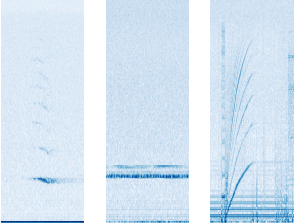
Example spectrograms of audio events found in the dataset, with time on the x-axis and frequency on the y-axis. Left: a humpback whale call (in particular, a tonal unit), Center: narrow-band noise from an unknown source, Right: hard disk noise from the HARP
This is a good representation for an image classifier, whose goal is to discriminate, because the different spectra (frequency decompositions) and time variations thereof (which are characteristic of distinct sound types) are represented in the spectrogram as visually dissimilar patterns. For the image model itself, we used ResNet-50, a convolutional neural network architecture typically used for image classification that has shown success at classifying non-speech audio. This is a supervised learning setup, where only manually labeled data could be used for training (0.2% of the entire dataset — in the next section, we describe an approach that makes use of the unlabeled data.)

The process of going from waveform to spectrogram involves choices of parameters and gain-scaling functions. Common default choices (one of which was logarithmic compression) were a good starting point, but some domain-specific tuning was needed to optimize the detection of whale calls. Humpback vocalizations are varied, but sustained, frequency-modulated, tonal units occur frequently in time. You can listen to an example below:


If the frequency didn't vary at all, a tonal unit would appear in the spectrogram as a horizontal bar. Since the calls are frequency-modulated, we actually see arcs instead of bars, but parts of the arcs are close to horizontal.

A challenge particular to this dataset was narrow-band noise, most often caused by nearby boats and the equipment itself. In a spectrogram it appears as horizontal lines, and early versions of the model would confuse it with humpback calls. This motivated us to try per-channel energy normalization (PCEN), which allows the suppression of stationary, narrow-band noise. This proved to be critical, providing a 24% reduction in error rate of whale call detection.
Spectrograms of the same 5-unit excerpt from humpback whale song beginning at 0:06 in the above recording. Top: PCEN. Bottom: log of squared magnitude. The dark blue horizontal bar along the bottom under log compression has become much lighter relative to the whale call when using PCEN
Aside from PCEN, averaging predictions over a longer period of time led to much better precision. This same effect happens for general audio event detection, but for humpback calls the increase in precision was surprisingly large. A likely explanation is that the vocalizations in our dataset are mainly in the context of whale song, a structured sequence of units than can last over 20 minutes. At the end of one unit in a song, there is a good chance another unit begins within two seconds. The input to the image model covers a short time window, but because the song is so long, model outputs from more distant time windows give extra information useful for making the correct prediction for the current time window.

Overall, evaluating on our test set of 75-second audio clips, the model identifies whether a clip contains humpback calls at over 90% precision and 90% recall. However, one should interpret these results with care; training and test data come from similar equipment and environmental conditions. That said, preliminary checks against some non-NOAA sources look promising.

Unsupervised Learning: Representation for Finding Similar Song Units
A different way to approach the question, "Where are all the humpback sounds in this data?", is to start with several examples of humpback sound and, for each of these, find more in the dataset that are similar to that example. The definition of similar here can be learned by the same ResNet we used when this was framed as a supervised problem. There, we used the labels to learn a classifier on top of the ResNet output. Here, we encourage a pair of ResNet output vectors to be close in Euclidean distance when the corresponding audio examples are close in time. With that distance function, we can retrieve many more examples of audio similar to a given one. In the future, this may be useful input for a classifier that distinguishes different humpback unit types from each other.

To learn the distance function, we used a method described in "Unsupervised Learning of Semantic Audio Representations", based on the idea that closeness in time is related to closeness in meaning. It randomly samples triplets, where each triplet is defined to consist of an anchor, a positive, and a negative. The positive and the anchor are sampled so that they start around the same time. An example of a triplet in our application would be a humpback unit (anchor), a probable repeat of the same unit by the same whale (positive) and background noise from some other month (negative). Passing the 3 samples through the ResNet (with tied weights) represents them as 3 vectors. Minimizing a loss that forces the anchor-negative distance to exceed the anchor-positive distance by a margin learns a distance function faithful to semantic similarity.

Principal component analysis (PCA) on a sample of labeled points lets us visualize the results. Separation between humpback and non-humpback is apparent. Explore for yourself using the TensorFlow Embedding Projector. Try changing Color by to each of class_label and site. Also, try changing PCA to t-SNE in the projector for a visualization that prioritizes preserving relative distances rather than sample variance.
A sample of 5000 data points in the unsupervised representation. (Orange: humpback. Blue: not humpback.)
Given individual "query" units, we retrieved the nearest neighbors in the entire corpus using Euclidean distance between embedding vectors. In some cases we found hundreds more instances of the same unit with good precision.
Manually chosen query units (boxed) and nearest neighbors using the unsupervised representation.
We intend to use these in the future to build a training set for a classifier that discriminates between song units. We could also use them to expand the training set used for learning a humpback detector.

Predictions from the Supervised Classifier on the Entire Dataset
We plotted summaries of the model output grouped by time and location. Not all sites had deployments in all years. Duty cycling (example: 5 minutes on, 15 minutes off) allows longer deployments on limited battery power, but the schedule can vary. To deal with these sources of variability, we consider the proportion of sampled time in which humpback calling was detected to the total time recorded in a month:
Time density of presence on year / month axes for the Kona and Saipan sites.
The apparent seasonal variation is consistent with a known pattern in which humpback populations spend summers feeding near Alaska and then migrate to the vicinity of the Hawaiian Islands to breed and give birth. This is a nice sanity check for the model.

We hope the predictions for the full dataset will equip experts at NOAA to reach deeper insights into the status of these populations and into the degree of any anthropogenic impacts on them. We also hope this is just one of the first few in a series of successes as Google works to accelerate the application of machine learning to the world's biggest humanitarian and environmental challenges.

Acknowledgements
We would like to thank Ann Allen (NOAA Fisheries) for providing the bulk of the ground truth data, for many useful rounds of feedback, and for some of the words in this post. Karlina Merkens (NOAA affiliate) provided further useful guidance. We also thank the NOAA Pacific Islands Fisheries Science Center as a whole for collecting and sharing the acoustic data.

Within Google, Jiayang Liu, Julie Cattiau, Aren Jansen, Rif A. Saurous, and Lauren Harrell contributed to this work. Special thanks go to Lauren, who designed the plots in the analysis section and implemented them using ggplot.

Source: Google AI Blog


Introducing the Kaggle “Quick, Draw!” Doodle Recognition Challenge


Online handwriting recognition consists of recognizing structured patterns in freeform handwritten input. While Google products like Translate, Keep and Handwriting Input use this technology to recognize handwritten text, it works for any predefined pattern for which enough training data is available. The same technology that lets you digitize handwritten text can also be used to improve your drawing abilities and build virtual worlds, and represents an exciting research direction that explores the potential of handwriting as a human-computer interaction modality. For example the “Quick, Draw!” game generated a dataset of 50M drawings (out of more than 1B that were drawn) which itself inspired many different new projects.

In order to encourage further research in this exciting field, we have launched the Kaggle "Quick, Draw!" Doodle Recognition Challenge, which tasks participants to build a better machine learning classifier for the existing “Quick, Draw!” dataset. Importantly, since the training data comes from the game itself (where drawings can be incomplete or may not match the label), this challenge requires the development of a classifier that can effectively learn from noisy data and perform well on a manually-labeled test set from a different distribution.

The Dataset
In the original “Quick, Draw!” game, the player is prompted to draw an image of a certain category (dog, cow, car, etc). The player then has 20 seconds to complete the drawing - if the computer recognizes the drawing correctly within that time, the player earns a point. Each game consists of 6 randomly chosen categories.
Because of the game mechanics, the labels in the Quick, Draw! dataset fall into the following categories:
  • Correct: the user drew the prompted category and the computer only recognized it correctly after the user was done drawing.
  • Correct, but incomplete: the user drew the prompted category and the computer recognized it correctly before the user had finished. Incompleteness can vary from nearly ready to only a fraction of the category drawn. This is probably fairly common in images that are marked as recognized correctly.
  • Correct, but not recognized correctly: The player drew the correct category but the AI never recognized it. Some players react to this by adding more details. Others scribble out and try again.
  • Incorrect: some players have different concepts in mind when they see a word - e.g. in the category seesaw, we have observed a number of saw drawings.
In addition to the labels described above, each drawing is given as a sequence of strokes, where each stroke is a sequence of touch points. While these can easily be rendered as images, using the order and direction of strokes often helps making handwriting recognizers better.

Get Started
We’ve previously published a tutorial that uses this dataset, and now we're inviting the community to build on this or other approaches to achieve even higher accuracy. You can get started by visiting the challenge website and going through the existing kernels which allow you to analyze the data and visualize it. We’re looking forward to learning about the approaches that the community comes up with for the competition and how much you can improve on our original production model.

Acknowledgements
We'd like to thank everyone who worked with us on this, particularly Jonas Jongejan and Brenda Fogg from the Creative Lab team, Julia Elliott and Walter Reade from the Kaggle team, and the handwriting recognition team.

Source: Google AI Blog


Scalable Deep Reinforcement Learning for Robotic Manipulation


How can robots acquire skills that generalize effectively to diverse, real-world objects and situations? While designing robotic systems that effectively perform repetitive tasks in controlled environments, like building products on an assembly line, is fairly routine, designing robots that can observe their surroundings and decide the best course of action while reacting to unexpected outcomes is exceptionally difficult. However, there are two tools that can help robots acquire such skills from experience: deep learning, which is excellent at handling unstructured real-world scenarios, and reinforcement learning, which enables longer-term reasoning while exhibiting more complex and robust sequential decision making. Combining these two techniques has the potential to enable robots to learn continuously from their experience, allowing them to master basic sensorimotor skills using data rather than manual engineering.

Designing reinforcement learning algorithms for robot learning introduces its own set of challenges: real-world objects span a wide variety of visual and physical properties, subtle differences in contact forces can make predicting object motion difficult and objects of interest can be obstructed from view. Furthermore, robotic sensors are inherently noisy, adding to the complexity. All of these factors makes it incredibly difficult to learn a general solution, unless there is enough variety in the training data, which takes time to collect. This motivates exploring learning algorithms that can effectively reuse past experience, similar to our previous work on grasping which benefited from large datasets. However, this previous work could not reason about the long-term consequences of its actions, which is important for learning how to grasp. For example, if multiple objects are clumped together, pushing one of them apart (called “singulation”) will make the grasp easier, even if doing so does not directly result in a successful grasp.
Examples of singulation.

To be more efficient, we need to use off-policy reinforcement learning, which can learn from data that was collected hours, days, or weeks ago. To design such an off-policy reinforcement learning algorithm that can benefit from large amounts of diverse experience from past interactions, we combined large-scale distributed optimization with a new fitted deep Q-learning algorithm that we call QT-Opt. A preprint is available on arXiv.

QT-Opt is a distributed Q-learning algorithm that supports continuous action spaces, making it well-suited to robotics problems. To use QT-Opt, we first train a model entirely offline, using whatever data we’ve already collected. This doesn’t require running the real robot, making it easier to scale. We then deploy and finetune that model on the real robot, further training it on newly collected data. As we run QT-Opt, we accumulate more offline data, letting us train better models, which lets us collect better data, and so on.

To apply this approach to robotic grasping, we used 7 real-world robots, which ran for 800 total robot hours over the course of 4 months. To bootstrap collection, we started with a hand-designed policy that succeeded 15-30% of the time. Data collection switched to the learned model when it started performing better. The policy takes a camera image and returns how the arm and gripper should move. The offline data contained grasps on over 1000 different objects.
Some of the training objects used.
In the past, we’ve seen that sharing experience across robots can accelerate learning. We scaled this training and data gathering process to ten GPUs, seven robots, and many CPUs, allowing us to collect and process a large dataset of over 580,000 grasp attempts. At the end of this process, we successfully trained a grasping policy that runs on a real world robot and generalizes to a diverse set of challenging objects that were not seen at training time.
Seven robots collecting grasp data.
Quantitatively, the QT-Opt approach succeeded in 96% of the grasp attempts across 700 trial grasps on previously unseen objects. Compared to our previous supervised-learning based grasping approach, which had a 78% success rate, our method reduced the error rate by more than a factor of five.
The objects used at evaluation time. To make the task challenging, we aimed for a large variety of object sizes, textures, and shapes.

Notably, the policy exhibits a variety of closed-loop, reactive behaviors that are often not found in standard robotic grasping systems:
  • When presented with a set of interlocking blocks that cannot be picked up together, the policy separates one of the blocks from the rest before picking it up.
  • When presented with a difficult-to-grasp object, the policy figures out it should reposition the gripper and regrasp it until it has a firm hold.
  • When grasping in clutter, the policy probes different objects until the fingers hold one of them firmly, before lifting.
  • When we perturbed the robot by intentionally swatting the object out of the gripper -- something it had not seen during training -- it automatically repositioned the gripper for another attempt.
Crucially, none of these behaviors were engineered manually. They emerged automatically from self-supervised training with QT-Opt, because they improve the model’s long-term grasp success.
Examples of the learned behaviors. In the left GIF, the policy corrects for the moved ball. In the right GIF, the policy tries several grasps until it succeeds at picking up the tricky object.

Additionally, we’ve found that QT-Opt reaches this higher success rate using less training data, albeit with taking longer to converge. This is especially exciting for robotics, where the bottleneck is usually collecting real robot data, rather than training time. Combining this with other data efficiency techniques (such as our prior work on domain adaptation for grasping) could open several interesting avenues in robotics. We’re also interested in combining QT-Opt with recent work on learning how to self-calibrate, which could further improve the generality.

Overall, the QT-Opt algorithm is a general reinforcement learning approach that’s giving us good results on real world robots. Besides the reward definition, nothing about QT-Opt is specific to robot grasping. We see this as a strong step towards more general robot learning algorithms, and are excited to see what other robotics tasks we can apply it to. You can learn more about this work in the short video below.
Acknowledgements
This research was conducted by Dmitry Kalashnikov, Alex Irpan, Peter Pastor, Julian Ibarz, Alexander Herzog, Eric Jang, Deirdre Quillen, Ethan Holly, Mrinal Kalakrishnan, Vincent Vanhoucke, and Sergey Levine. We’d also like to give special thanks to Iñaki Gonzalo and John-Michael Burke for overseeing the robot operations, Chelsea Finn, Timothy Lillicrap, and Arun Nair for valuable discussions, and other people at Google and X who’ve contributed their expertise and time towards this research. A preprint is available on arXiv.

Source: Google AI Blog


How Can Neural Network Similarity Help Us Understand Training and Generalization?


In order to solve tasks, deep neural networks (DNNs) progressively transform input data into a sequence of complex representations (i.e., patterns of activations across individual neurons). Understanding these representations is critically important, not only for interpretability, but also so that we can more intelligently design machine learning systems. However, understanding these representations has proven quite difficult, especially when comparing representations across networks. In a previous post, we outlined the benefits of Canonical Correlation Analysis (CCA) as a tool for understanding and comparing the representations of convolutional neural networks (CNNs), showing that they converge in a bottom-up pattern, with early layers converging to their final representations before later layers over the course of training.

In “Insights on Representational Similarity in Neural Networks with Canonical Correlation” we develop this work further to provide new insights into the representational similarity of CNNs, including differences between networks which memorize (e.g., networks which can only classify images they have seen before) from those which generalize (e.g., networks which can correctly classify previously unseen images). Importantly, we also extend this method to provide insights into the dynamics of recurrent neural networks (RNNs), a class of models that are particularly useful for sequential data, such as language. Comparing RNNs is difficult in many of the same ways as CNNs, but RNNs present the additional challenge that their representations change over the course of a sequence. This makes CCA, with its helpful invariances, an ideal tool for studying RNNs in addition to CNNs. As such, we have additionally open sourced the code used for applying CCA on neural networks with the hope that will help the research community better understand network dynamics.

Representational Similarity of Memorizing and Generalizing CNNs
Ultimately, a machine learning system is only useful if it can generalize to new situations it has never seen before. Understanding the factors which differentiate between networks that generalize and those that don’t is therefore essential, and may lead to new methods to improve generalization performance. To investigate whether representational similarity is predictive of generalization, we studied two types of CNNs:
  • generalizing networks: CNNs trained on data with unmodified, accurate labels and which learn solutions which generalize to novel data.
  • memorizing networks: CNNs trained on datasets with randomized labels such that they must memorize the training data and cannot, by definition, generalize (as in Zhang et al., 2017).
We trained multiple instances of each network, differing only in the initial randomized values of the network weights and the order of the training data, and used a new weighted approach to calculate the CCA distance measure (see our paper for details) to compare the representations within each group of networks and between memorizing and generalizing networks.

We found that groups of different generalizing networks consistently converged to more similar representations (especially in later layers) than groups of memorizing networks (see figure below). At the softmax, which denotes the network’s ultimate prediction, the CCA distance for each group of generalizing and memorizing networks decreases substantially, as the networks in each separate group make similar predictions.
Groups of generalizing networks (blue) converge to more similar solutions than groups of memorizing networks (red). CCA distance was calculated between groups of networks trained on real CIFAR-10 labels (“Generalizing”) or randomized CIFAR-10 labels (“Memorizing”) and between pairs of memorizing and generalizing networks (“Inter”).
Perhaps most surprisingly, in later hidden layers, the representational distance between any given pair of memorizing networks was about the same as the representational distance between a memorizing and generalizing network (“Inter” in the plot above), despite the fact that these networks were trained on data with entirely different labels. Intuitively, this result suggests that while there are many different ways to memorize the training data (resulting in greater CCA distances), there are fewer ways to learn generalizable solutions. In future work, we plan to explore whether this insight can be used to regularize networks to learn more generalizable solutions.

Understanding the Training Dynamics of Recurrent Neural Networks
So far, we have only applied CCA to CNNs trained on image data. However, CCA can also be applied to calculate representational similarity in RNNs, both over the course of training and over the course of a sequence. Applying CCA to RNNs, we first asked whether the RNNs exhibit the same bottom-up convergence pattern we observed in our previous work for CNNs. To test this, we measured the CCA distance between the representation at each layer of the RNN over the course of training with its final representation at the end of training. We found that the CCA distance for layers closer to the input dropped earlier in training than for deeper layers, demonstrating that, like CNNs, RNNs also converge in a bottom-up pattern (see figure below).
Convergence dynamics for RNNs over the course of training exhibit bottom up convergence, as layers closer to the input converge to their final representations earlier in training than later layers. For example, layer 1 converges to its final representation earlier in training than layer 2 than layer 3 and so on. Epoch designates the number of times the model has seen the entire training set while different colors represent the convergence dynamics of different layers.
Additional findings in our paper show that wider networks (e.g., networks with more neurons at each layer) converge to more similar solutions than narrow networks. We also found that trained networks with identical structures but different learning rates converge to distinct clusters with similar performance, but highly dissimilar representations. We also apply CCA to RNN dynamics over the course of a single sequence, rather than simply over the course of training, providing some initial insights into the various factors which influence RNN representations over time.

Conclusions
These findings reinforce the utility of analyzing and comparing DNN representations in order to provide insights into network function, generalization, and convergence. However, there are still many open questions: in future work, we hope to uncover which aspects of the representation are conserved across networks, both in CNNs and RNNs, and whether these insights can be used to improve network performance. We encourage others to try out the code used for the paper to investigate what CCA can tell us about other neural networks!

Acknowledgements
Special thanks to Samy Bengio, who is a co-author on this work. We also thank Martin Wattenberg, Jascha Sohl-Dickstein and Jon Kleinberg for helpful comments.

Source: Google AI Blog