Tag Archives: machine learning

Giving Lens New Reading Capabilities in Google Go


Around the world, millions of people are coming online for the first time, and many of them are among the 800 million adults worldwide who are unable to read or write, or those who are migrating to towns and cities where they are not able to speak the predominant language. As a smartphone camera-based tool, Google Lens has great potential for helping people who struggle with reading and other language-based challenges. Lens uses computer vision, machine learning and Google’s Knowledge Graph to let people turn the things they see in the real world into a visual search box, enabling them to identify objects like plants and animals, or to copy and paste text from the real world into their phone.

However, in order for Lens to be able to help the greatest number of people, we needed to create a special version that can work on even the most basic smartphones. So at I/O 2019, we announced a new version of Lens designed specifically for use in Google Go—our Search app for entry level devices—and we included a new set of features designed to help people who face reading and other language-based challenges. When users point their camera at text they don’t understand, Lens in Google Go can translate and read it out loud. It even highlights each word as it’s being read so users can follow along. If you want to try out these features for yourself, they are available today via Lens in Google Go. While Google Go was initially available only on Android Go devices and on the Google Play Store in select markets, recently, we made it available globally in the Google Play Store.
To make these reading features work, the Google Go version of Lens needs to be able to capture high quality images on a wide variety of devices, then identify the text, understand its structure, translate and overlay it in context, and finally, read it out loud.

Image Capture
Image capture on entry-level devices, like those that run Android Go, is tricky since it must work on a wide variety of devices, many of which are more resource constrained than flagship phones. To build a universal tool that can reliably capture high-quality images with minimal lag, we made Lens in Google Go an early adopter of a new Android support library called CameraX. Available in Jetpack—a suite of libraries, tools, and guidance for Android developers—CameraX is an abstraction layer over the Android Camera2 API that resolves device compatibility issues so developers don't have to write their own device-specific code.

Using CameraX, we implemented two capture strategies to balance capture latency against performance impact. On higher-end phones, which are powerful enough to provide a constant stream of high-resolution frames from which to select an image, we’ve made capture instantaneous. On less advanced devices, streaming these frames could cause camera lag since the CPU is less powerful, so we process the frame when the user taps capture to produce a single, on-demand high-resolution image.

Text Recognition
After Lens in Google Go captures an image, it needs to make sense of the shapes and letters that constitute the words, sentences and paragraphs. To do this, the image is scaled down and transferred to the Lens server, where the processing will be performed. Next, optical character recognition (OCR) is applied, which utilizes a region proposal network to detect character level bounding boxes that can be merged into lines for text recognition.
Merging these character boxes into words is a two-step, sequential process. The first step is to apply the Hough Transform, which assumes the text is distributed across parallel lines. The second step uses Text Flow, which instead traces text that may follow a curve by finding the shortest path through a graph of detected text boxes. This ensures that text with a variety of distributions, be they straight, curved or mixed, can be identified and processed.

Because the images captured by Lens in Google Go may include sources such as signage, handwriting or documents, a slew of additional challenges can arise. For example, the text can be obscured, scripts can be uniquely stylized, and images can be blurry. All of these issues can cause the OCR engine to misunderstand various characters within each word. To correct mistakes and improve word accuracy, Lens in Google Go uses the context of surrounding words to make corrections. It also utilizes the Knowledge Graph to provide contextual clues, such as whether a word is likely a proper noun and should not be spell-corrected.

All of these steps, from script detection and direction identification to text recognition, are performed by separable convolutional neural networks (CNNs) with an additional quantized long short-term memory (LSTM) network. And the models are trained on data from a variety of sources, ranging from ReCaptcha to scanned images from Google Books.
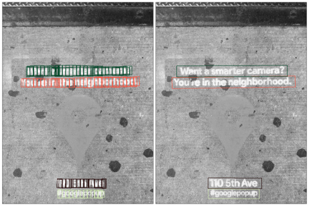
Left: Image with bounding box around recognized text. The raw OCR output from this image reads, “Cise is beauti640”. Right: By applying Knowledge Graph in addition to context from nearby words, Lens in Google Go recognizes the words, “life is beautiful”.
Understanding Structure
Once the individual words have been recognized, Lens must determine how to fit them together. The text that people come across in the real world is laid out in many different ways. A newspaper, for example, is laid out into columns, with headlines, article text, and advertisements. Meanwhile, a bus schedule, has one column for destinations and another with times. While understanding text structure comes very naturally to people, computers need to be taught how to comprehend it. Lens uses CNNs to detect coherent text blocks like columns, or text in a consistent style or color. And then, within each block, it uses signals like text-alignment, language, and the geometric relationship of the paragraphs to determine their final reading order.

One of the other challenges in detecting document structure is that people take pictures of text from different angles, often with a warped perspective. This means we cannot revert to off-the-shelf detectors that rely on axis aligned boxes, but must generalize our systems to be able to deal with homographic distortions.
Paragraph segmentation on the front page of a newspaper. Notice how “News Analysis”, which is embedded in the middle of a column, has been identified separately due to its distinct style features.
Translations in Context
To provide users with the most helpful information, translations must be both accurate and contextual. Lens uses Google Translate’s neural machine translation (NMT) algorithms, to translate entire sentences at a time, rather than going word-by-word, in order to preserve proper grammar and diction.

For the translation to be most useful, it needs to be placed in the context of the original text. For example, when translating instructions on an ATM, it is important to know which buttons correspond to which instructions. Part of the challenge is accounting for the fact that the translated text can be much shorter or longer than the original. For example, German sentences tend to be longer than English ones. To accomplish this seamless overlay, Lens redistributes the translation into lines of similar length, and chooses an appropriate font size to match. It also matches the color of the translation and its background with the original text through the use of a heuristic that assumes the background and the text differ in luminosity, and that the background takes up the majority of the space. This allows Lens to classify whether a pixel represents background or text, and then sample the average color from these two regions to ensure the translated text matches the original text.

Reading the Text Out Loud
The final challenge in delivering information in the most helpful way with Lens in Google Go is reading the text aloud. High-fidelity audio is generated using Google Text-to-Speech (TTS), a service that applies machine learning to disambiguate and detected entities such as dates, phone numbers and addresses, and uses that to generate realistic speech based on DeepMind’s WaveNet.

These reading features become more contextual and useful when they are paired with display. Lens utilizes timing annotations from the TTS service that mark the beginning of each word in order to highlight each word on screen as it’s being read, similar to a karaoke machine. Say for example, a user takes a picture of an ATM screen with different labels next to different buttons. This karaoke effect allows users to know which label applies to which button. It may also help users learn how to pronounce the words being translated.
Looking Ahead
Taken together, it is our hope that these features will have a positive impact on the day-to-day lives of millions of people. Moving forward, we will continue to work on further updates to these reading features to make the OCR more precise, including improvements to text structure understanding (e.g. multi-column text) and recognition of Indic scripts. As we address these text challenges, we continue to look for new ways that the combination of machine learning and the smartphone camera can help people as they go about their lives.

Source: Google AI Blog


Exploring Weight Agnostic Neural Networks


When training a neural network to accomplish a given task, be it image classification or reinforcement learning, one typically refines a set of weights associated with each connection within the network. Another approach to creating successful neural networks that has shown substantial progress is neural architecture search, which constructs neural network architectures out of hand-engineered components such as convolutional network components or transformer blocks. It has been shown that neural network architectures built with these components, such as deep convolutional networks, have strong inductive biases for image processing tasks, and can even perform them when their weights are randomly initialized. While neural architecture search produces new ways of arranging hand-engineered components with known inductive biases for the task domain at hand, there has been little progress in the automated discovery of new neural network architectures with such inductive biases, for various task domains.

We can look at analogies to these useful components in examples of nature vs. nurture. Just as certain precocial species in biology—who possess anti-predator behaviors from the moment of birth—can perform complex motor and sensory tasks without learning, perhaps we can construct network architectures that can perform well without training. Of course, these natural (and by analogy, artificial) neural networks are further improved through training, but their ability to perform even without learning shows that they contain biases that make them well-suited to their task.

In “Weight Agnostic Neural Networks” (WANN), we present a first step toward searching specifically for networks with these biases: neural net architectures that can already perform various tasks, even when they use a random shared weight. Our motivation in this work is to question to what extent neural network architectures alone, without learning any weight parameters, can encode solutions for a given task. By exploring such neural network architectures, we present agents that can already perform well in their environment without the need to learn weight parameters. Furthermore, in order to spur progress in this field community, we have also open-sourced the code to reproduce our WANN experiments for the broader research community.
Left: A hand-engineered, fully-connected deep neural network with 2760 weight connections. Using a learning algorithm, we can solve for the set of 2760 weight parameters so that this network can perform the BipedalWalker-v2 task. Right: A weight agnostic neural network architecture with 44 connections that can perform the same Bipedal Walker task. Unlike the fully-connected network, this WANN can still perform the task without the need to train the weight parameters of each connection. In fact, to simplify the training, the WANN is designed to perform when the values of each weight connection are identical, or shared, and it will even function if this shared weight parameter is randomly sampled.
Finding WANNs
We start with a population of minimal neural network architecture candidates, each with very few connections only, and use a well-established topology search algorithm (NEAT), to evolve the architectures by adding single connections and single nodes one by one. The key idea behind WANNs is to search for architectures by de-emphasizing weights. Unlike traditional neural architecture search methods, where all of the weight parameters of new architectures need to be trained using a learning algorithm, we take a simpler and more efficient approach. Here, during the search, all candidate architectures are first assigned a single shared weight value at each iteration, and then optimized to perform well over a wide range of shared weight values.
Operators for searching the space of network topologies
Left: A minimal network topology, with input and outputs only partially connected.
Middle: Networks are altered in one of three ways:
(1) Insert Node: a new node is inserted by splitting an existing connection.
(2) Add Connection: a new connection is added by connecting two previously unconnected nodes.
(3) Change Activation: the activation function of a hidden node is reassigned.
Right: Possible activation functions (linear, step, sin, cosine, Gaussian, tanh, sigmoid, inverse, absolute value, ReLU)
In addition to exploring a range of weight agnostic neural networks, it is important to also look for network architectures that are only as complex as they need to be. We accomplish this by optimizing for both the performance of the networks and their complexity simultaneously, using techniques drawn from multi-objective optimization.
Overview of Weight Agnostic Neural Network Search and corresponding operators for searching the space of network topologies.
Training WANN Architectures
Unlike traditional networks, we can easily train the WANN by simply finding the best single shared weight parameter that maximizes its performance. In the example below, we see that our architecture works (to some extent) for a swing-up cartpole task using constant weights:
A WANN performing a Cartpole Swing-up task at various different weight parameters, and also using fine-tuned weight parameters.
As we see in the above figure, while WANNs can perform its task using range of shared weight parameters, the performance is still not comparable to a network that learns weights for each individual connection, as normally done in network training. If we want to further improve its performance, we can use the WANN architecture, and the best shared weight as a starting point to fine-tune the weights of each individual connection using a learning algorithm, like how we would normally train any neural network. Using the weight agnostic property of the network architecture as a starting point, and fine-tuning its performance via learning, may help provide insightful analogies to how animals learn.
Through the use of multi-objective optimization for both performance and network simplicity, our method found a simple WANN for a Car Racing from pixels task that works well without explicitly training for the weights of the network.
The ability for a network architecture to function using only random weights offers other advantages too. For instance, by using copies of the same WANN architecture, but where each copy of the WANN is assigned a different distinct weight value, we can create an ensemble of multiple distinct models for the same task. This ensemble generally achieves better performance than a single model. We illustrate this with an example of an MNIST classifier evolved to work with random weights:
An MNIST classifier evolved to work with random weights.
While a conventional network with random initialization will achieve ~10% accuracy on MNIST, this particular network architecture uses random weights and when applied to MNIST achieves an accuracy much better than chance (> 80%). When an ensemble of WANNs is used, each of which assigned with a different shared weight, the accuracy increases to > 90%.

Even without ensemble methods, collapsing the number of weight values in a network to one allows the network to be rapidly tuned. The ability to quickly fine-tune weights might be useful in continual lifelong learning, where agents acquire, adapt, and transfer skills throughout their lifespan. This makes WANNs particularly well positioned to exploit the Baldwin effect, the evolutionary pressure that rewards individuals predisposed to learn useful behaviors, without being trapped in the computationally expensive trap of ‘learning to learn’.

Conclusion
We hope that this work can serve as a stepping stone to help discover novel fundamental neural network components such as the convolutional network, whose discovery and application have been instrumental to the incredible progress made in deep learning. The computational resources available to the research community have grown significantly since the time convolutional neural networks were discovered. If we are devoting such resources to automated discovery and hope to achieve more than incremental improvements in network architectures, we believe it is also worth searching for with new building blocks, not just their arrangements.

If you are interested to learn more about this work, we invite readers to read our interactive article (or pdf version of the paper for offline reading). In addition to open sourcing these experiments to the research community, we have also released a general Python implementation of NEAT called PrettyNEAT to help interested readers to explore the exciting area of neural network evolution from first principles.

Source: Google AI Blog


Bi-Tempered Logistic Loss for Training Neural Nets with Noisy Data


The quality of models produced by machine learning (ML) algorithms directly depends on the quality of the training data, but real world datasets typically contain some amount of noise that introduces challenges for ML models. Noise in the dataset can take several forms from corrupted examples (e.g., lens flare in an image of a cat) to mislabelled examples from when the data was collected (e.g., an image of cat mislabelled as a flerken).

The ability of an ML model to deal with noisy training data depends in great part on the loss function used in the training process. For classification tasks, the standard loss function used for training is the logistic loss. However, this particular loss function falls short when handling noisy training examples due to two unfortunate properties:
  1. Outliers far away can dominate the overall loss: The logistic loss function is sensitive to outliers. This is because the loss function value grows without bound as the mislabelled examples (outliers) are far away from the decision boundary. Thus, a single bad example that is located far away from the decision boundary can penalize the training process to the extent that the final trained model learns to compensate for it by stretching the decision boundary and potentially sacrificing the remaining good examples. This “large-margin” noise issue is illustrated in the left panel of the figure below.
  2. Mislabeled examples nearby can stretch the decision boundary: The output of the neural network is a vector of activation values, which reflects the margin between the example and the decision boundary for each class. The softmax transfer function is used to convert the activation values into probabilities that an example will belong to each class. As the tail of this transfer function for the logistic loss decays exponentially fast, the training process will tend to stretch the boundary closer to a mislabeled example in order to compensate for its small margin. Consequently, the generalization performance of the network will immediately deteriorate, even with a low level of label noise (right panel below).
We visualize the decision surface of a 2-layered neural network as it is trained for binary classification. Blue and orange dots represent the examples from the two classes. The network is trained with logistic loss under two types of noisy conditions: (left) large-margin noise and (right) small-margin-noise.
We tackle these two problems in a recent paper by introducing a “bi-tempered” generalization of the logistic loss endowed with two tunable parameters that handle those situations well, which we call “temperatures”—t1, which characterizes boundedness, and t2 for tail-heaviness (i.e. the rate of decline in the tail of the transfer function). These properties are illustrated below. Setting both t1 and t2 to 1.0 recovers the logistic loss function. Setting t1 lower than 1.0 increases the boundedness and setting t2 greater than 1.0 makes for a heavier-tailed transfer function. We also introduce this interactive visualization which allows you to visualize the neural network training process with the bi-tempered logistic loss.
Left: Boundedness of the loss function. When t1 is between 0 and 1, exclusive, only a finite amount of loss is incurred for each example, even if they are mislabeled. Shown is t1 = 0.8. Right: Tail-heaviness of the transfer function. The heavy-tailed transfer function applies when t2 = > 1.0 and assigns higher probability for the same amount of activation, thus preventing the boundary from drawing closer to the noisy example. Shown is t2 = 2.0.
To demonstrate the effect of each temperature, we train a two-layer feed-forward neural network for a binary classification problem on a synthetic dataset that contains a circle of points from the first class, and a concentric ring of points from the second class. You can try this yourself on your browser with our interactive visualization. We use the standard logistic loss function, which can be recovered by setting both temperatures equal to 1.0, as well as our bi-tempered logistic loss for training the network. We then demonstrate the effects of each loss function for a clean dataset, a dataset with small-margin noise, large-margin noise, and a dataset with random noise.
Logistic vs. bi-tempered logistic loss: (a) noise-free labels, (b) small-margin label noise, (c) large-margin label noise, and (d) random label noise. The temperature values (t1, t2) for the tempered loss are shown above each figure. We find that for each situation, the decision boundary recovered by training with the bi-tempered logistic loss function is better than before.
Noise Free Case:
We show the results of training the model on the noise-free dataset in column (a), using the logistic loss (top) and the bi-tempered logistic loss (bottom). The white line shows the decision boundary for each model. The values of (t1, t2), the temperatures in the bi-tempered loss function, are shown below each column of the figure. Notice that for this choice of temperatures, the loss is bounded and the transfer function is tail-heavy. As can be seen, both losses produce good decision boundaries that successfully separates the two classes.

Small-Margin Noise:
To illustrate the effect of tail-heaviness of the probabilities, we artificially corrupt a random subset of the examples that are near the decision boundary, that is, we flip the labels of these points to the opposite class. The results of training the networks on data with small-margin noise using the logistic loss as well as the bi-tempered loss is shown in column (b).

As can be seen, the logistic loss, due to the lightness of the softmax tail, stretches the boundary closer to the noisy points to compensate for their low probabilities. On the other hand, the bi-tempered loss using only the tail-heavy probability transfer function by adjusting t2 can successfully avoid the noisy examples. This can be explained by the heavier tail of the tempered exponential function, which assigns reasonably high probability values (and thus, keeps the loss value small) while maintaining the decision boundary away from the noisy examples.

Large-Margin Noise:
Next, we evaluate the performance of the two loss functions for handling large-margin noisy examples. In (c), we randomly corrupt a subset of the examples that are located far away from the decision boundary, the outer side of the ring as well as points near the center).

For this case, we only use the boundedness property of the bi-tempered loss, while keeping the softmax probabilities the same as the logistic loss. The unboundedness of the logistic loss causes the decision boundary to expand towards the noisy points to reduce their loss values. On the other hand, the bounded bi-tempered loss, bounded by adjusting t1, incurs a finite amount of loss for each noisy example. As a result, the bi-tempered loss can avoid these noisy examples and maintain a good decision boundary.

Random Noise:
Finally, we investigate the effect of random noise in the training data on the two loss functions. Note that random noise comprises both small-margin and large-margin noisy examples. Thus, we use both boundedness and tail-heaviness properties of the bi-tempered loss function by setting the temperatures to (t1, t2) = (0.2, 4.0).

As can be seen from the results in the last column, (d), the logistic loss is highly affected by the noisy examples and clearly fails to converge to a good decision boundary. On the other hand, the bi-tempered can recover a decision boundary that is almost identical to the noise-free case.

Conclusion
In this work we constructed a bounded, tempered loss function that can handle large-margin outliers and introduced heavy-tailedness in our new tempered softmax function, which can handle small-margin mislabeled examples. Using our bi-tempered logistic loss, we achieve excellent empirical performance on training neural networks on a number of large standard datasets (please see our paper for full details). Note that the state-of-the-art neural networks have been optimized along with a large variety of variables such as: architecture, transfer function, choice of optimizer, and label smoothing to name just a few. Our method introduces two additional tunable variables, namely (t1, t2). We believe that with a systematic “joint optimization” of all commonly tried variables, significant further improvements can be achieved in conjunction with our loss function. This is of course a more long-term goal. We also plan to explore the idea of annealing the temperature parameters over the training process.

Acknowledgements:
This blogpost reflects work with our co-authors Manfred Warmuth, Visiting Researcher and Tomer Koren, Senior Research Scientist, Google Research. Preprint of our paper is available here, which contains theoretical analysis of the loss function and empirical results on standard datasets at scale.

Source: Google AI Blog


Coral summer updates: Post-training quant support, TF Lite delegate, and new models!

Posted by Vikram Tank (Product Manager), Coral Team

Summer updates cartoon

Coral’s had a busy summer working with customers, expanding distribution, and building new features — and of course taking some time for R&R. We’re excited to share updates, early work, and new models for our platform for local AI with you.

The compiler has been updated to version 2.0, adding support for models built using post-training quantization—only when using full integer quantization (previously, we required quantization-aware training)—and fixing a few bugs. As the Tensorflow team mentions in their Medium post “post-training integer quantization enables users to take an already-trained floating-point model and fully quantize it to only use 8-bit signed integers (i.e. `int8`).” In addition to reducing the model size, models that are quantized with this method can now be accelerated by the Edge TPU found in Coral products.

We've also updated the Edge TPU Python library to version 2.11.1 to include new APIs for transfer learning on Coral products. The new on-device back propagation API allows you to perform transfer learning on the last layer of an image classification model. The last layer of a model is removed before compilation and implemented on-device to run on the CPU. It allows for near-real time transfer learning and doesn’t require you to recompile the model. Our previously released imprinting API, has been updated to allow you to quickly retrain existing classes or add new ones while leaving other classes alone. You can now even keep the classes from the pre-trained base model. Learn more about both options for on-device transfer learning.

Until now, accelerating your model with the Edge TPU required that you write code using either our Edge TPU Python API or in C++. But now you can accelerate your model on the Edge TPU when using the TensorFlow Lite interpreter API, because we've released a TensorFlow Lite delegate for the Edge TPU. The TensorFlow Lite Delegate API is an experimental feature in TensorFlow Lite that allows for the TensorFlow Lite interpreter to delegate part or all of graph execution to another executor—in this case, the other executor is the Edge TPU. Learn more about the TensorFlow Lite delegate for Edge TPU.

Coral has also been working with Edge TPU and AutoML teams to release EfficientNet-EdgeTPU: a family of image classification models customized to run efficiently on the Edge TPU. The models are based upon the EfficientNet architecture to achieve the image classification accuracy of a server-side model in a compact size that's optimized for low latency on the Edge TPU. You can read more about the models’ development and performance on the Google AI Blog, and download trained and compiled versions on the Coral Models page.

And, as summer comes to an end we also want to share that Arrow offers a student teacher discount for those looking to experiment with the boards in class or the lab this year.

We're excited to keep evolving the Coral platform, please keep sending us feedback at [email protected].

Learning Better Simulation Methods for Partial Differential Equations


The world’s fastest supercomputers were designed for modeling physical phenomena, yet they still are not fast enough to robustly predict the impacts of climate change, to design controls for airplanes based on airflow or to accurately simulate a fusion reactor. All of these phenomena are modeled by partial differential equations (PDEs), the class of equations that describe everything smooth and continuous in the physical world, and the most common class of simulation problems in science and engineering. To solve these equations, we need faster simulations, but in recent years, Moore’s law has been slowing. At the same time, we’ve seen huge breakthroughs in machine learning (ML) along with faster hardware optimized for it. What does this new paradigm offer for scientific computing?

In “Learning Data Driven Discretizations for Partial Differential Equations”, published in Proceedings of the National Academy of Sciences, we explore a potential path for how ML can offer continued improvements in high-performance computing, both for solving PDEs and, more broadly, for solving hard computational problems in every area of science.

For most real-world problems, closed-form solutions to PDEs don’t exist. Instead, one must find discrete equations (“discretizations”) that a computer can solve to approximate the continuous PDE. Typical approaches to solve PDEs represent equations on a grid, e.g., using finite differences. To achieve convergence, the mesh spacing of the grid needs to be smaller than the smallest feature size of the solutions. This often isn’t feasible because of an unfortunate scaling law: achieving 10x higher resolution requires 10,000x more compute, because the grid must be scaled in four dimensions—three spatial dimensions and time. Instead, in our paper we show that ML can be used to learn better representations for PDEs on coarser grids.
Satellite photo of a hurricane, at both full resolution and simulated resolution in a state of the art weather model. Cumulus clouds (e.g., in the red circle) are responsible for heavy rainfall, but in the weather model the details are entirely blurred out. Instead, models rely on crude approximations for sub-grid physics, a key source of uncertainty in climate models. Image credit: NOAA
The challenge is to retain the accuracy of high-resolution simulations while still using the coarsest grid possible. In our work we’re able to improve upon existing schemes by replacing heuristics based on deep human insight (e.g., “solutions to a PDE should always be smooth away from discontinuities”) with optimized rules based on machine learning. The rules our ML models recover are complex, and we don’t entirely understand them, but they incorporate sophisticated physical principles like the idea of “upwinding”—to accurately model what’s coming towards you in a fluid flow, you should look upstream in the direction the wind is coming from. An example of our results on a simple model of fluid dynamics are shown below:
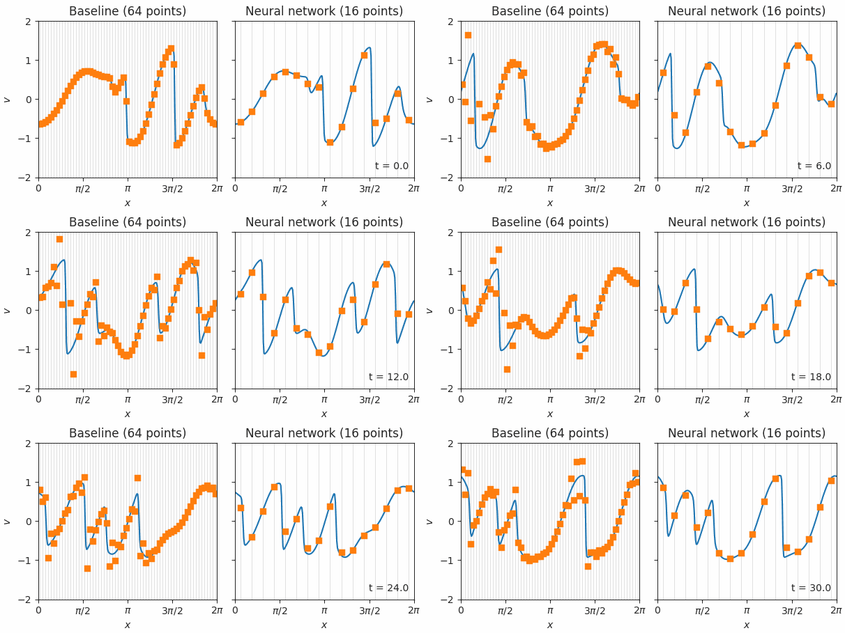
Simulations of Burgers’ equation, a model for shock waves in fluids, solved with either a standard finite volume method (left) or our neural network based method (right). The orange squares represent simulations with each method on low resolution grids. These points are fed back into the model at each time step, which then predicts how they should change. Blue lines show the exact simulations used for training. The neural network solution is much better, even on a 4x coarser grid, as indicated by the orange squares smoothly tracing the blue line.
Our research also illustrates a broader lesson about how to effectively combine machine learning and physics. Rather than attempting to learn physics from scratch, we combined neural networks with components from traditional simulation methods, including the known form of the equations we’re solving and finite volume methods. This means that laws such as conservation of momentum are exactly satisfied, by construction, and allows our machine learning models to focus on what they do best, learning optimal rules for interpolation in complex, high-dimensional spaces.

Next Steps
We are focused on scaling up the techniques outlined in our paper to solve larger scale simulation problems with real-world impacts, such as weather and climate prediction. We’re excited about the broad potential of blending machine learning into the complex algorithms of scientific computing.

Acknowledgments
Thanks to co-authors Yohai Bar-Sinari, Jason Hickey and Michael Brenner; and Google collaborators Peyman Milanfar, Pascal Getreur, Ignacio Garcia Dorado, Dmitrii Kochkov, Jiawei Zhuang and Anton Geraschenko.

Source: Google AI Blog


Innovations in Graph Representation Learning


Relational data representing relationships between entities is ubiquitous on the Web (e.g., online social networks) and in the physical world (e.g., in protein interaction networks). Such data can be represented as a graph with nodes (e.g., users, proteins), and edges connecting them (e.g., friendship relations, protein interactions). Given the widespread prevalence of graphs, graph analysis plays a fundamental role in machine learning, with applications in clustering, link prediction, privacy, and others. To apply machine learning methods to graphs (e.g., predicting new friendships, or discovering unknown protein interactions) one needs to learn a representation of the graph that is amenable to be used in ML algorithms.

However, graphs are inherently combinatorial structures made of discrete parts like nodes and edges, while many common ML methods, like neural networks, favor continuous structures, in particular vector representations. Vector representations are particularly important in neural networks, as they can be directly used as input layers. To get around the difficulties in using discrete graph representations in ML, graph embedding methods learn a continuous vector space for the graph, assigning each node (and/or edge) in the graph to a specific position in a vector space. A popular approach in this area is that of random-walk-based representation learning, as introduced in DeepWalk.

Left: The well-known Karate graph representing a social network. Right: A continuous space embedding of the nodes in the graph using DeepWalk.
Here we present the results of two recent papers on graph embedding: “Is a Single Embedding Enough? Learning Node Representations that Capture Multiple Social Contexts” presented at WWW’19 and “Watch Your Step: Learning Node Embeddings via Graph Attention” at NeurIPS’18. The first paper introduces a novel technique to learn multiple embeddings per node, enabling a better characterization of networks with overlapping communities. The second addresses the fundamental problem of hyperparameter tuning in graph embeddings, allowing one to easily deploy graph embeddings methods with less effort. We are also happy to announce that we have released the code for both papers in the Google Research github repository for graph embeddings.

Learning Node Representations that Capture Multiple Social Contexts
In virtually all cases, the crucial assumption of standard graph embedding methods is that a single embedding has to be learned for each node. Thus, the embedding method can be said to seek to identify the single role or position that characterizes each node in the geometry of the graph. Recent work observed, however, that nodes in real networks belong to multiple overlapping communities and play multiple roles—think about your social network where you participate in both your family and in your work community. This observation motivates the following research question: is it possible to develop methods where nodes are embedded in multiple vectors, representing their participation in overlapping communities?

In our WWW’19 paper, we developed Splitter, an unsupervised embedding method that allows the nodes in a graph to have multiple embeddings to better encode their participation in multiple communities. Our method is based on recent innovations in overlapping clustering based on ego-network analysis, using the persona graph concept, in particular. This method takes a graph G, and creates a new graph P (called the persona graph), where each node in G is represented by a series of replicas called the persona nodes. Each persona of a node represents an instantiation of the node in a local community to which it belongs. For each node U in the graph, we analyze the ego-network of the node (i.e., the graph connecting the node to its neighbors, in this example A, B, C, D) to discover local communities to which the node belongs. For instance, in the figure below, node U belongs to two communities: Cluster 1 (with the friends A and B, say U’s family members) and Cluster 2 (with C and D, say U’s colleagues).
Ego-net of node U
Then, we use this information to “split” node U into its two personas U1 (the family persona) and U2 (the work persona). This disentangles the two communities, so that they no longer overlap.
The ego-splitting method separating the U nodes in 2 personas.
This technique has been used to improve the state-of-the-art results in graph embedding methods, showing up to 90% reduction in link prediction (i.e., predicting which link will form in the future) error on a variety of graphs. The key reason for this improvement is the ability of the method to disambiguate highly overlapping communities found in social networks and other real-world graphs. We further validate this result with an in-depth analysis of co-authorship graphs where authors belong to overlapping research communities (e.g., machine learning and data mining).
Top Left: A typical graphs with highly overlapping communities. Top Right: A traditional embedding of the graph on the left using node2vec. Bottom Left: A persona graph of the graph above. Bottom Right: The Splitter embedding of the persona graph. Notice how the persona graph clearly disentangles the overlapping communities of the original graph and Splitter outputs well-separated embeddings.
Automatic hyper-parameter tuning via graph attention.
Graph embedding methods have shown outstanding performance on various ML-based applications, such as link prediction and node classification, but they have a number of hyper-parameters that must be manually set. For example, are nearby nodes more important to capture when learning embeddings than nodes that are further away? Even though experts may be able to fine tune these hyper-parameters, one must do so independently for each graph. To obviate such manual work, in our second paper, we proposed a method to learn the optimal hyper-parameters automatically.

Specifically, many graph embedding methods, like DeepWalk, employ random walks to explore the context around a given node (i.e. the direct neighbors, the neighbors of the neighbors, etc). Such random walks can have many hyper-parameters that allow tuning of the local exploration of the graph, thus regulating the attention given by the embeddings to nearby nodes. Different graphs may present different optimal attention patterns and hence different optimal hyperparameters (see the picture below, where we show two different attention distributions). Watch Your Step formulates a model for the performance of the embedding methods based on the above mentioned hyper-parameters. Then we optimize the hyper-parameters to maximize the performance predicted by the model, using standard backpropagation. We found that the values learned by backpropagation agree with the optimal hyper-parameters obtained by grid search.
Our new method for automatic hyper-parameter tuning, Watch Your Step, uses an attention model to learn different graph context distributions. Shown above are two example local neighborhoods about a center node (in yellow) and the context distributions (red gradient) that was learned by the model. The left-side graph shows a more diffused attention model, while the distribution on the right shows one concentrated on direct neighbors.
This work falls under the growing family of AutoML, where we want to alleviate the burden of optimizing the hyperparameters—a common problem in practical machine learning. Many AutoML methods use neural architecture search. This paper instead shows a variant, where we use the mathematical connection between the hyperparameters in the embeddings and graph-theoretic matrix formulations. The “Auto” portion corresponds to learning the graph hyperparameters by backpropagation.

We believe that our contributions will further advance the state of the research in graph embedding in various directions. Our method for learning multiple node embeddings draws a connection between the rich and well-studied field of overlapping community detection, and the more recent one of graph embedding which we believe may result in fruitful future research. An open problem in this area is the use of multiple-embedding methods for classification. Furthermore, our contribution on learning hyperparameters will foster graph embedding adoption by reducing the need for expensive manual tuning. We hope the release of these papers and code will help the research community pursue these directions.

Acknowledgements
We thank Sami Abu-el-Haija who contributed to this work and is now a Ph.D. student at USC.

Source: Google AI Blog


Introducing TensorNetwork, an Open Source Library for Efficient Tensor Calculations

Originally posted on the Google AI Blog.

Many of the world's toughest scientific challenges, like developing high-temperature superconductors and understanding the true nature of space and time, involve dealing with the complexity of quantum systems. What makes these challenges difficult is that the number of quantum states in these systems is exponentially large, making brute-force computation infeasible. To deal with this, data structures called tensor networks are used. Tensor networks let one focus on the quantum states that are most relevant for real-world problems—the states of low energy, say—while ignoring other states that aren't relevant. Tensor networks are also increasingly finding applications in machine learning (ML). However, there remain difficulties that prohibit them from widespread use in the ML community: 1) a production-level tensor network library for accelerated hardware has not been available to run tensor network algorithms at scale, and 2) most of the tensor network literature is geared toward physics applications and creates the false impression that expertise in quantum mechanics is required to understand the algorithms.

In order to address these issues, we are releasing TensorNetwork, a brand new open source library to improve the efficiency of tensor calculations, developed in collaboration with the Perimeter Institute for Theoretical Physics and X. TensorNetwork uses TensorFlow as a backend and is optimized for GPU processing, which can enable speedups of up to 100x when compared to work on a CPU. We introduce TensorNetwork in a series of papers, the first of which presents the new library and its API, and provides an overview of tensor networks for a non-physics audience. In our second paper we focus on a particular use case in physics, demonstrating the speedup that one gets using GPUs.

How are Tensor Networks Useful?

Tensors are multidimensional arrays, categorized in a hierarchy according to their order: e.g., an ordinary number is a tensor of order zero (also known as a scalar), a vector is an order-one tensor, a matrix is an order-two tensorDiagrammatic notation for tensors. and so on. While low-order tensors can easily be represented by an explicit array of numbers or with a mathematical symbol such as Tijnklm (where the number of indices represents the order of the tensor), that notation becomes very cumbersome once we start talking about high-order tensors. At that point it's useful to start using diagrammatic notation, where one simply draws a circle (or some other shape) with a number of lines, or legs, coming out of it—the number of legs being the same as the order of the tensor. In this notation, a scalar is just a circle, a vector has a single leg, a matrix has two legs, etc. Each leg of the tensor also has a dimension, which is the size of that leg. For example, a vector representing an object's velocity through space would be a three-dimensional, order-one tensor.
Diagrammatic notation for tensors.
The benefit of representing tensors in this way is to succinctly encode mathematical operations, e.g., multiplying a matrix by a vector to produce another vector, or multiplying two vectors to make a scalar. These are all examples of a more general concept called tensor contraction.
Diagrammatic notation for tensor contraction. Vector and matrix multiplication, as well as the matrix trace (i.e., the sum of the diagonal elements of a matrix), are all examples.
These are also simple examples of tensor networks, which are graphical ways of encoding the pattern of tensor contractions of several constituent tensors to form a new one. Each constituent tensor has an order determined by its own number of legs. Legs that are connected, forming an edge in the diagram, represent contraction, while the number of remaining dangling legs determines the order of the resultant tensor.
Left: The trace of the product of four matrices, tr(ABCD), which is a scalar. You can see that it has no dangling legs. Right: Three order-three tensors being contracted with three legs dangling, resulting in a new order-three tensor.
While these examples are very simple, the tensor networks of interest often represent hundreds of tensors contracted in a variety of ways. Describing such a thing would be very obscure using traditional notation, which is why the diagrammatic notation was invented by Roger Penrose in 1971.

Tensor Networks in Practice

Consider a collection of black-and-white images, each of which can be thought of as a list of N pixel values. A single pixel of a single image can be one-hot-encoded into a two-dimensional vector, and by combining these pixel encodings together we can make a 2N-dimensional one-hot encoding of the entire image. We can reshape that high-dimensional vector into an order-N tensor, and then add up all of the tensors in our collection of images to get a total tensor Ti1,i2,...,iN encapsulating the collection.
This sounds like a very wasteful thing to do: encoding images with about 50 pixels in this way would already take petabytes of memory. That's where tensor networks come in. Rather than storing or manipulating the tensor T directly, we instead represent T as the contraction of many smaller constituent tensors in the shape of a tensor network. That turns out to be much more efficient. For instance, the popular matrix product state (MPS) network would write T in terms of N much smaller tensors, so that the total number of parameters is only linear in N, rather than exponential.
The high-order tensor T is represented in terms of many low-order tensors in a matrix product state tensor network.
It's not obvious that large tensor networks can be efficiently created or manipulated while consistently avoiding the need for a huge amount of memory. But it turns out that this is possible in many cases, which is why tensor networks have been used extensively in quantum physics and, now, in machine learning. Stoudenmire and Schwab used the encoding just described to make an image classification model, demonstrating a new use for tensor networks. The TensorNetwork library is designed to facilitate exactly that kind of work, and our first paper describes how the library functions for general tensor network manipulations.

Performance in Physics Use-Cases

TensorNetwork is a general-purpose library for tensor network algorithms, and so it should prove useful for physicists as well. Approximating quantum states is a typical use-case for tensor networks in physics, and is well-suited to illustrate the capabilities of the TensorNetwork library. In our second paper, we describe a tree tensor network (TTN) algorithm for approximating the ground state of either a periodic quantum spin chain (1D) or a lattice model on a thin torus (2D), and implement the algorithm using TensorNetwork. We compare the use of CPUs with GPUs and observe significant computational speed-ups, up to a factor of 100, when using a GPU and the TensorNetwork library.
Computational time as a function of the bond dimension, χ. The bond dimension determines the size of the constituent tensors of the tensor network. A larger bond dimension means the tensor network is more powerful, but requires more computational resources to manipulate.

Conclusion and Future Work

These are the first in a series of planned papers to illustrate the power of TensorNetwork in real-world applications. In our next paper we will use TensorNetwork to classify images in the MNIST and Fashion-MNIST datasets. Future plans include time series analysis on the ML side, and quantum circuit simulation on the physics side. With the open source community, we are also always adding new features to TensorNetwork itself. We hope that TensorNetwork will become a valuable tool for physicists and machine learning practitioners.

Acknowledgements

The TensorNetwork library was developed by Chase Roberts, Adam Zalcman, and Bruce Fontaine of Google AI; Ashley Milsted, Martin Ganahl, and Guifre Vidal of the Perimeter Institute; and Jack Hidary and Stefan Leichenauer of X. We'd also like to thank Stavros Efthymiou at X for valuable contributions.

by Chase Roberts, Research Engineer, Google AI and Stefan Leichenauer, Research Scientist, X 

Introducing Google Research Football: A Novel Reinforcement Learning Environment


The goal of reinforcement learning (RL) is to train smart agents that can interact with their environment and solve complex tasks, with real-world applications towards robotics, self-driving cars, and more. The rapid progress in this field has been fueled by making agents play games such as the iconic Atari console games, the ancient game of Go, or professionally played video games like Dota 2 or Starcraft 2, all of which provide challenging environments where new algorithms and ideas can be quickly tested in a safe and reproducible manner. The game of football is particularly challenging for RL, as it requires a natural balance between short-term control, learned concepts, such as passing, and high level strategy.

Today we are happy to announce the release of the Google Research Football Environment, a novel RL environment where agents aim to master the world’s most popular sport—football. Modeled after popular football video games, the Football Environment provides a physics based 3D football simulation where agents control either one or all football players on their team, learn how to pass between them, and manage to overcome their opponent’s defense in order to score goals. The Football Environment provides several crucial components: a highly-optimized game engine, a demanding set of research problems called Football Benchmarks, as well as the Football Academy, a set of progressively harder RL scenarios. In order to facilitate research, we have released a beta version of the underlying open-source code on Github.

Football Engine
The core of the Football Environment is an advanced football simulation, called Football Engine, which is based on a heavily modified version of Gameplay Football. Based on input actions for the two opposing teams, it simulates a match of football including goals, fouls, corner and penalty kicks, and offsides. The Football Engine is written in highly optimized C++ code, allowing it to be run on off-the-shelf machines, both with GPU and without GPU-based rendering enabled. This allows it to reach a performance of approximately 25 million steps per day on a single hexa-core machine.
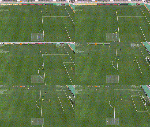
The Football Engine is an advanced football simulation that supports all the major football rules such as kickoffs (top left), goals (top right), fouls, cards (bottom left), corner and penalty kicks (bottom right), and offside.
The Football Engine has additional features geared specifically towards RL. First, it allows learning from both different state representations, which contain semantic information such as the player’s locations, as well as learning from raw pixels. Second, to investigate the impact of randomness, it can be run in both a stochastic mode (enabled by default), in which there is randomness in both the environment and opponent AI actions, and in a deterministic mode, where there is no randomness. Third, the Football Engine is out of the box compatible with the widely used OpenAI Gym API. Finally, researchers can get a feeling for the game by playing against each other or their agents, using either keyboards or gamepads.

Football Benchmarks
With the Football Benchmarks, we propose a set of benchmark problems for RL research based on the Football Engine. The goal in these benchmarks is to play a “standard” game of football against a fixed rule-based opponent that was hand-engineered for this purpose. We provide three versions: the Football Easy Benchmark, the Football Medium Benchmark, and the Football Hard Benchmark, which only differ in the strength of the opponent.

As a reference, we provide benchmark results for two state-of-the-art reinforcement learning algorithms: DQN and IMPALA, which both can be run in multiple processes on a single machine or concurrently on many machines. We investigate both the setting where the only rewards provided to the algorithm are the goals scored and the setting where we provide additional rewards for moving the ball closer to the goal.

Our results indicate that the Football Benchmarks are interesting research problems of varying difficulties. In particular, the Football Easy Benchmark appears to be suitable for research on single-machine algorithms while the Football Hard Benchmark proves to be challenging even for massively distributed RL algorithms. Based on the nature of the environment and the difficulty of the benchmarks, we expect them to be useful for investigating current scientific challenges such as sample-efficient RL, sparse rewards, or model based RL.
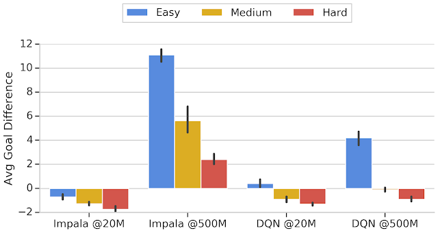
The average goal difference of agent versus opponent at different difficulty levels for different baselines. The Easy opponent can be beaten by a DQN agent trained for 20 million steps, while the Medium and Hard opponents require a distributed algorithm such as IMPALA that is trained for 200 million steps.
Football Academy & Future Directions
As training agents for the full Football Benchmarks can be challenging, we also provide Football Academy, a diverse set of scenarios of varying difficulty. This allows researchers to get the ball rolling on new research ideas, allows testing of high-level concepts (such as passing), and provides a foundation to investigate curriculum learning research ideas, where agents learn from progressively harder scenarios. Examples of the Football Academy scenarios include settings where agents have to learn how to score against the empty goal, where they have to learn how to quickly pass between players, and where they have to learn how to execute a counter-attack. Using a simple API, researchers can further define their own scenarios and train agents to solve them.

Top: A successful policy that runs towards the goal (as required, since a number of opponents chase our player) and scores against the goal-keeper. Second: A beautiful way to drive and finish a counter-attack. Third: A simple way to solve a 2-vs-1 play. Bottom: The agent scores after a corner kick.
The Football Benchmarks and the Football Academy consider the standard RL setup, in which agents compete against a fixed opponent, i.e., where the opponent can be considered a part of the environment. Yet, in reality, football is a two-player game where two different teams compete and where one has to adapt to the actions and strategy of the opposing team. The Football Engine provides a unique opportunity for research into this setting and, once we complete our on-going effort to implement self-play, even more interesting research settings can be investigated.

Acknowledgments
This project was undertaken together with Anton Raichuk, Piotr Stańczyk, Michał Zając, Lasse Espeholt, Carlos Riquelme, Damien Vincent‎, Marcin Michalski, Olivier Bousquet‎ and Sylvain Gelly at Google Research, Zürich. We also wish to thank Lucas Beyer, Nal Kalchbrenner, Tim Salimans and the rest of the Google Brain team for helpful discussions, comments, technical help and code contributions. Finally, we would like to thank Bastiaan Konings Schuiling, who authored and open-sourced the original version of this game.

Source: Google AI Blog


Introducing TensorNetwork, an Open Source Library for Efficient Tensor Calculations


Many of the world's toughest scientific challenges, like developing high-temperature superconductors and understanding the true nature of space and time, involve dealing with the complexity of quantum systems. What makes these challenges difficult is that the number of quantum states in these systems is exponentially large, making brute-force computation infeasible. To deal with this, data structures called tensor networks are used. Tensor networks let one focus on the quantum states that are most relevant for real-world problems—the states of low energy, say—while ignoring other states that aren't relevant. Tensor networks are also increasingly finding applications in machine learning (ML). However, there remain difficulties that prohibit them from widespread use in the ML community: 1) a production-level tensor network library for accelerated hardware has not been available to run tensor network algorithms at scale, and 2) most of the tensor network literature is geared toward physics applications and creates the false impression that expertise in quantum mechanics is required to understand the algorithms.

In order to address these issues, we are releasing TensorNetwork, a brand new open source library to improve the efficiency of tensor calculations, developed in collaboration with the Perimeter Institute for Theoretical Physics and X. TensorNetwork uses TensorFlow as a backend and is optimized for GPU processing, which can enable speedups of up to 100x when compared to work on a CPU. We introduce TensorNetwork in a series of papers, the first of which presents the new library and its API, and provides an overview of tensor networks for a non-physics audience. In our second paper we focus on a particular use case in physics, demonstrating the speedup that one gets using GPUs.

How are Tensor Networks Useful?
Tensors are multidimensional arrays, categorized in a hierarchy according to their order: e.g., an ordinary number is a tensor of order zero (also known as a scalar), a vector is an order-one tensor, a matrix is an order-two tensor, and so on. While low-order tensors can easily be represented by an explicit array of numbers or with a mathematical symbol such as Tijnklm (where the number of indices represents the order of the tensor), that notation becomes very cumbersome once we start talking about high-order tensors. At that point it’s useful to start using diagrammatic notation, where one simply draws a circle (or some other shape) with a number of lines, or legs, coming out of it—the number of legs being the same as the order of the tensor. In this notation, a scalar is just a circle, a vector has a single leg, a matrix has two legs, etc. Each leg of the tensor also has a dimension, which is the size of that leg. For example, a vector representing an object’s velocity through space would be a three-dimensional, order-one tensor.


Diagrammatic notation for tensors.
The benefit of representing tensors in this way is to succinctly encode mathematical operations, e.g., multiplying a matrix by a vector to produce another vector, or multiplying two vectors to make a scalar. These are all examples of a more general concept called tensor contraction.

Diagrammatic notation for tensor contraction. Vector and matrix multiplication, as well as the matrix trace (i.e., the sum of the diagonal elements of a matrix), are all examples.
These are also simple examples of tensor networks, which are graphical ways of encoding the pattern of tensor contractions of several constituent tensors to form a new one. Each constituent tensor has an order determined by its own number of legs. Legs that are connected, forming an edge in the diagram, represent contraction, while the number of remaining dangling legs determines the order of the resultant tensor.
Left: The trace of the product of four matrices, tr(ABCD), which is a scalar. You can see that it has no dangling legs. Right: Three order-three tensors being contracted with three legs dangling, resulting in a new order-three tensor.
While these examples are very simple, the tensor networks of interest often represent hundreds of tensors contracted in a variety of ways. Describing such a thing would be very obscure using traditional notation, which is why the diagrammatic notation was invented by Roger Penrose in 1971.

Tensor Networks in Practice
Consider a collection of black-and-white images, each of which can be thought of as a list of N pixel values. A single pixel of a single image can be one-hot-encoded into a two-dimensional vector, and by combining these pixel encodings together we can make a 2N-dimensional one-hot encoding of the entire image. We can reshape that high-dimensional vector into an order-N tensor, and then add up all of the tensors in our collection of images to get a total tensor Ti1,i2,...,iN encapsulating the collection.

This sounds like a very wasteful thing to do: encoding images with about 50 pixels in this way would already take petabytes of memory. That’s where tensor networks come in. Rather than storing or manipulating the tensor T directly, we instead represent T as the contraction of many smaller constituent tensors in the shape of a tensor network. That turns out to be much more efficient. For instance, the popular matrix product state (MPS) network would write T in terms of N much smaller tensors, so that the total number of parameters is only linear in N, rather than exponential.
The high-order tensor T is represented in terms of many low-order tensors in a matrix product state tensor network.
It’s not obvious that large tensor networks can be efficiently created or manipulated while consistently avoiding the need for a huge amount of memory. But it turns out that this is possible in many cases, which is why tensor networks have been used extensively in quantum physics and, now, in machine learning. Stoudenmire and Schwab used the encoding just described to make an image classification model, demonstrating a new use for tensor networks. The TensorNetwork library is designed to facilitate exactly that kind of work, and our first paper describes how the library functions for general tensor network manipulations.

Performance in Physics Use-Cases
TensorNetwork is a general-purpose library for tensor network algorithms, and so it should prove useful for physicists as well. Approximating quantum states is a typical use-case for tensor networks in physics, and is well-suited to illustrate the capabilities of the TensorNetwork library. In our second paper, we describe a tree tensor network (TTN) algorithm for approximating the ground state of either a periodic quantum spin chain (1D) or a lattice model on a thin torus (2D), and implement the algorithm using TensorNetwork. We compare the use of CPUs with GPUs and observe significant computational speed-ups, up to a factor of 100, when using a GPU and the TensorNetwork library.
Computational time as a function of the bond dimension, χ. The bond dimension determines the size of the constituent tensors of the tensor network. A larger bond dimension means the tensor network is more powerful, but requires more computational resources to manipulate.
Conclusion and Future Work
These are the first in a series of planned papers to illustrate the power of TensorNetwork in real-world applications. In our next paper we will use TensorNetwork to classify images in the MNIST and Fashion-MNIST datasets. Future plans include time series analysis on the ML side, and quantum circuit simulation on the physics side. With the open source community, we are also always adding new features to TensorNetwork itself. We hope that TensorNetwork will become a valuable tool for physicists and machine learning practitioners.

Acknowledgements
The TensorNetwork library was developed by Chase Roberts, Adam Zalcman, and Bruce Fontaine of Google AI; Ashley Milsted, Martin Ganahl, and Guifre Vidal of the Perimeter Institute; and Jack Hidary and Stefan Leichenauer of X. We’d also like to thank Stavros Efthymiou at X for valuable contributions.

Source: Google AI Blog


Coral updates: Project tutorials, a downloadable compiler, and a new distributor

Posted by Vikram Tank (Product Manager), Coral Team

coral hardware

We’re committed to evolving Coral to make it even easier to build systems with on-device AI. Our team is constantly working on new product features, and content that helps ML practitioners, engineers, and prototypers create the next generation of hardware.

To improve our toolchain, we're making the Edge TPU Compiler available to users as a downloadable binary. The binary works on Debian-based Linux systems, allowing for better integration into custom workflows. Instructions on downloading and using the binary are on the Coral site.

We’re also adding a new section to the Coral site that showcases example projects you can build with your Coral board. For instance, Teachable Machine is a project that guides you through building a machine that can quickly learn to recognize new objects by re-training a vision classification model directly on your device. Minigo shows you how to create an implementation of AlphaGo Zero and run it on the Coral Dev Board or USB Accelerator.

Our distributor network is growing as well: Arrow will soon sell Coral products.