Understanding sequential data — such as language, music or videos — is a challenging task, especially when there is dependence on extensive surrounding context. For example, if a person or an object disappears from view in a video only to re-appear much later, many models will forget how it looked. In the language domain, long short-term memory (LSTM) neural networks cover enough context to translate sentence-by-sentence. In this case, the context window (i.e., the span of data taken into consideration in the translation) covers from dozens to about a hundred words. The more recent Transformer model not only improved performance in sentence-by-sentence translation, but could be used to generate entire Wikipedia articles through multi-document summarization. This is possible because the context window used by Transformer extends to thousands of words. With such a large context window, Transformer could be used for applications beyond text, including pixels or musical notes, enabling it to be used to generate music and images.
However, extending Transformer to even larger context windows runs into limitations. The power of Transformer comes from attention, the process by which it considers all possible pairs of words within the context window to understand the connections between them. So, in the case of a text of 100K words, this would require assessment of 100K x 100K word pairs, or 10 billion pairs for each step, which is impractical. Another problem is with the standard practice of storing the output of each model layer. For applications using large context windows, the memory requirement for storing the output of multiple model layers quickly becomes prohibitively large (from gigabytes with a few layers to terabytes in models with thousands of layers). This means that realistic Transformer models, using numerous layers, can only be used on a few paragraphs of text or generate short pieces of music.
Today, we introduce the Reformer, a Transformer model designed to handle context windows of up to 1 million words, all on a single accelerator and using only 16GB of memory. It combines two crucial techniques to solve the problems of attention and memory allocation that limit Transformer’s application to long context windows. Reformer uses locality-sensitive-hashing (LSH) to reduce the complexity of attending over long sequences and reversible residual layers to more efficiently use the memory available.
The Attention Problem
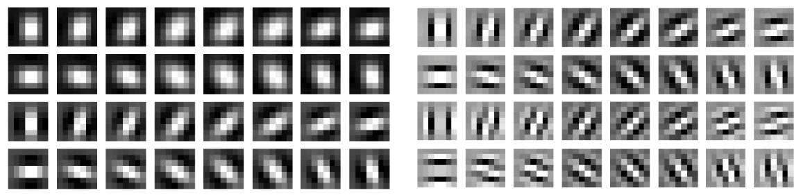
The first challenge when applying a Transformer model to a very large text sequence is how to handle the attention layer. LSH accomplishes this by computing a hash function that matches similar vectors together, instead of searching through all possible pairs of vectors. For example, in a translation task, where each vector from the first layer of the network represents a word (even larger contexts in subsequent layers), vectors corresponding to the same words in different languages may get the same hash. In the figure below, different colors depict different hashes, with similar words having the same color. When the hashes are assigned, the sequence is rearranged to bring elements with the same hash together and divided into segments (or chunks) to enable parallel processing. Attention is then applied within these much shorter chunks (and their adjoining neighbors to cover the overflow), greatly reducing the computational load.
 |
| Locality-sensitive-hashing: Reformer takes in an input sequence of keys, where each key is a vector representing individual words (or pixels, in the case of images) in the first layer and larger contexts in subsequent layers. LSH is applied to the sequence, after which the keys are sorted by their hash and chunked. Attention is applied only within a single chunk and its immediate neighbors. |
While LSH solves the problem with attention, there is still a memory issue. A single layer of a network often requires up to a few GB of memory and usually fits on a single GPU, so even a model with long sequences could be executed if it only had one layer. But when training a multi-layer model with gradient descent, activations from each layer need to be saved for use in the backward pass. A typical Transformer model has a dozen or more layers, so memory quickly runs out if used to cache values from each of those layers.
The second novel approach implemented in Reformer is to recompute the input of each layer on-demand during back-propagation, rather than storing it in memory. This is accomplished by using reversible layers, where activations from the last layer of the network are used to recover activations from any intermediate layer, by what amounts to running the network in reverse. In a typical residual network, each layer in the stack keeps adding to vectors that pass through the network. Reversible layers, instead, have two sets of activations for each layer. One follows the standard procedure just described and is progressively updated from one layer to the next, but the other captures only the changes to the first. Thus, to run the network in reverse, one simply subtracts the activations applied at each layer.
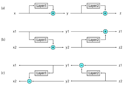 |
| Reversible layers: (A) In a standard residual network, the activations from each layer are used to update the inputs into the next layer. (B) In a reversible network, two sets of activations are maintained, only one of which is updated after each layer. (C) This approach enables running the network in reverse in order to recover all intermediate values. |
The novel application of these two approaches in Reformer makes it highly efficient, enabling it to process text sequences of lengths up to 1 million words on a single accelerator using only 16GB of memory. Since Reformer has such high efficiency, it can be applied directly to data with context windows much larger than virtually all current state-of-the-art text domain datasets. Perhaps Reformer’s ability to deal with such large datasets will stimulate the community to create them.
One area where there is no shortage of large-context data is image generation, so we experiment with the Reformer on images. In this colab, we present examples of how Reformer can be used to “complete” partial images. Starting with the image fragments shown in the top row of the figure below, Reformer can generate full frame images (bottom row), pixel-by-pixel.
 |
| Top: Image fragments used as input to Reformer. Bottom: “Completed” full-frame images. Original images are from the Imagenet64 dataset. |
Conclusion
We believe Reformer gives the basis for future use of Transformer models, both for long text and applications outside of natural language processing. Following our tradition of doing research in the open, we have already started exploring how to apply it to even longer sequences and how to improve handling of positional encodings. Read the Reformer paper (selected for oral presentation at ICLR 2020), explore our code and develop your own ideas too. Few long-context datasets are widely used in deep learning yet, but in the real world long context is everywhere. Maybe you can find a new application for Reformer — start with this colab and chat with us if you have any problems or questions!
Acknowledgements
This research was conducted by Nikita Kitaev, Łukasz Kaiser and Anselm Levskaya. Additional thanks go to Afroz Mohiuddin, Jonni Kanerva and Piotr Kozakowski for their work on Trax and to the whole JAX team for their support.


 Posted by