Tag Archives: Audio

SoundStorm: Efficient parallel audio generation

Posted by Zalán Borsos, Research Software Engineer, and Marco Tagliasacchi, Senior Staff Research Scientist, Google Research

The recent progress in generative AI unlocked the possibility of creating new content in several different domains, including text, vision and audio. These models often rely on the fact that raw data is first converted to a compressed format as a sequence of tokens. In the case of audio, neural audio codecs (e.g., SoundStream or EnCodec) can efficiently compress waveforms to a compact representation, which can be inverted to reconstruct an approximation of the original audio signal. Such a representation consists of a sequence of discrete audio tokens, capturing the local properties of sounds (e.g., phonemes) and their temporal structure (e.g., prosody). By representing audio as a sequence of discrete tokens, audio generation can be performed with Transformer-based sequence-to-sequence models — this has unlocked rapid progress in speech continuation (e.g., with AudioLM), text-to-speech (e.g., with SPEAR-TTS), and general audio and music generation (e.g., AudioGen and MusicLM). Many generative audio models, including AudioLM, rely on auto-regressive decoding, which produces tokens one by one. While this method achieves high acoustic quality, inference (i.e., calculating an output) can be slow, especially when decoding long sequences.

To address this issue, in “SoundStorm: Efficient Parallel Audio Generation”, we propose a new method for efficient and high-quality audio generation. SoundStorm addresses the problem of generating long audio token sequences by relying on two novel elements: 1) an architecture adapted to the specific nature of audio tokens as produced by the SoundStream neural codec, and 2) a decoding scheme inspired by MaskGIT, a recently proposed method for image generation, which is tailored to operate on audio tokens. Compared to the autoregressive decoding approach of AudioLM, SoundStorm is able to generate tokens in parallel, thus decreasing the inference time by 100x for long sequences, and produces audio of the same quality and with higher consistency in voice and acoustic conditions. Moreover, we show that SoundStorm, coupled with the text-to-semantic modeling stage of SPEAR-TTS, can synthesize high-quality, natural dialogues, allowing one to control the spoken content (via transcripts), speaker voices (via short voice prompts) and speaker turns (via transcript annotations), as demonstrated by the examples below:

Input: Text (transcript used to drive the audio generation in bold)	Something really funny happened to me this morning. \| Oh wow, what? \| Well, uh I woke up as usual. \| Uhhuh \| Went downstairs to have uh breakfast. \| Yeah \| Started eating. Then uh 10 minutes later I realized it was the middle of the night. \| Oh no way, that's so funny!	I didn't sleep well last night. \| Oh, no. What happened? \| I don't know. I I just couldn't seem to uh to fall asleep somehow, I kept tossing and turning all night. \| That's too bad. Maybe you should uh try going to bed earlier tonight or uh maybe you could try reading a book. \| Yeah, thanks for the suggestions, I hope you're right. \| No problem. I I hope you get a good night's sleep

Input: Audio prompt

Output: Audio prompt + generated audio

SoundStorm design

In our previous work on AudioLM, we showed that audio generation can be decomposed into two steps: 1) semantic modeling, which generates semantic tokens from either previous semantic tokens or a conditioning signal (e.g., a transcript as in SPEAR-TTS, or a text prompt as in MusicLM), and 2) acoustic modeling, which generates acoustic tokens from semantic tokens. With SoundStorm we specifically address this second, acoustic modeling step, replacing slower autoregressive decoding with faster parallel decoding.

SoundStorm relies on a bidirectional attention-based Conformer, a model architecture that combines a Transformer with convolutions to capture both local and global structure of a sequence of tokens. Specifically, the model is trained to predict audio tokens produced by SoundStream given a sequence of semantic tokens generated by AudioLM as input. When doing this, it is important to take into account the fact that, at each time step t, SoundStream uses up to Q tokens to represent the audio using a method known as residual vector quantization (RVQ), as illustrated below on the right. The key intuition is that the quality of the reconstructed audio progressively increases as the number of generated tokens at each step goes from 1 to Q.

At inference time, given the semantic tokens as input conditioning signal, SoundStorm starts with all audio tokens masked out, and fills in the masked tokens over multiple iterations, starting from the coarse tokens at RVQ level q = 1 and proceeding level-by-level with finer tokens until reaching level q = Q.

There are two crucial aspects of SoundStorm that enable fast generation: 1) tokens are predicted in parallel during a single iteration within a RVQ level and, 2) the model architecture is designed in such a way that the complexity is only mildly affected by the number of levels Q. To support this inference scheme, during training a carefully designed masking scheme is used to mimic the iterative process used at inference.

SoundStorm model architecture. T denotes the number of time steps and Q the number of RVQ levels used by SoundStream. The semantic tokens used as conditioning are time-aligned with the SoundStream frames.

Measuring SoundStorm performance

We demonstrate that SoundStorm matches the quality of AudioLM's acoustic generator, replacing both AudioLM's stage two (coarse acoustic model) and stage three (fine acoustic model). Furthermore, SoundStorm produces audio 100x faster than AudioLM's hierarchical autoregressive acoustic generator (top half below) with matching quality and improved consistency in terms of speaker identity and acoustic conditions (bottom half below).

Runtimes of SoundStream decoding, SoundStorm and different stages of AudioLM on a TPU-v4.

Acoustic consistency between the prompt and the generated audio. The shaded area represents the inter-quartile range.

Safety and risk mitigation

We acknowledge that the audio samples produced by the model may be influenced by the unfair biases present in the training data, for instance in terms of represented accents and voice characteristics. In our generated samples, we demonstrate that we can reliably and responsibly control speaker characteristics via prompting, with the goal of avoiding unfair biases. A thorough analysis of any training data and its limitations is an area of future work in line with our responsible AI Principles.

In turn, the ability to mimic a voice can have numerous malicious applications, including bypassing biometric identification and using the model for the purpose of impersonation. Thus, it is crucial to put in place safeguards against potential misuse: to this end, we have verified that the audio generated by SoundStorm remains detectable by a dedicated classifier using the same classifier as described in our original AudioLM paper. Hence, as a component of a larger system, we believe that SoundStorm would be unlikely to introduce additional risks to those discussed in our earlier papers on AudioLM and SPEAR-TTS. At the same time, relaxing the memory and computational requirements of AudioLM would make research in the domain of audio generation more accessible to a wider community. In the future, we plan to explore other approaches for detecting synthesized speech, e.g., with the help of audio watermarking, so that any potential product usage of this technology strictly follows our responsible AI Principles.

Conclusion

We have introduced SoundStorm, a model that can efficiently synthesize high-quality audio from discrete conditioning tokens. When compared to the acoustic generator of AudioLM, SoundStorm is two orders of magnitude faster and achieves higher temporal consistency when generating long audio samples. By combining a text-to-semantic token model similar to SPEAR-TTS with SoundStorm, we can scale text-to-speech synthesis to longer contexts and generate natural dialogues with multiple speaker turns, controlling both the voices of the speakers and the generated content. SoundStorm is not limited to generating speech. For example, MusicLM uses SoundStorm to synthesize longer outputs efficiently (as seen at I/O).

Acknowledgments

The work described here was authored by Zalán Borsos, Matt Sharifi, Damien Vincent, Eugene Kharitonov, Neil Zeghidour and Marco Tagliasacchi. We are grateful for all discussions and feedback on this work that we received from our colleagues at Google.

Source: Google AI Blog

Who Said What? Recorder’s On-device Solution for Labeling Speakers

Posted by Quan Wang, Senior Staff Software Engineer, and Fan Zhang, Staff Software Engineer, Google

In 2019 we launched Recorder, an audio recording app for Pixel phones that helps users create, manage, and edit audio recordings. It leverages recent developments in on-device machine learning to transcribe speech, recognize audio events, suggest tags for titles, and help users navigate transcripts.

Nonetheless, some Recorder users found it difficult to navigate long recordings that have multiple speakers because it's not clear who said what. During the Made By Google event this year, we announced the "speaker labels" feature for the Recorder app. This opt-in feature annotates a recording transcript with unique and anonymous labels for each speaker (e.g., "Speaker 1", "Speaker 2", etc.) in real time during the recording. It significantly improves the readability and usability of the recording transcripts. This feature is powered by Google's new speaker diarization system named Turn-to-Diarize, which was first presented at ICASSP 2022.

Left: Recorder transcript without speaker labels. Right: Recorder transcript with speaker labels.

System Architecture

Our speaker diarization system leverages several highly optimized machine learning models and algorithms to allow diarizing hours of audio in a real-time streaming fashion with limited computational resources on mobile devices. The system mainly consists of three components: a speaker turn detection model that detects a change of speaker in the input speech, a speaker encoder model that extracts voice characteristics from each speaker turn, and a multi-stage clustering algorithm that annotates speaker labels to each speaker turn in a highly efficient way. All components run fully on the device.

Architecture of the Turn-to-Diarize system.

Detecting Speaker Turns

The first component of our system is a speaker turn detection model based on a Transformer Transducer (T-T), which converts the acoustic features into text transcripts augmented with a special token <st> representing a speaker turn. Unlike preceding customized systems that use role-specific tokens (e.g., <doctor> and <patient>) for conversations, this model is more generic and can be trained on and deployed to various application domains.

In most applications, the output of a diarization system is not directly shown to users, but combined with a separate automatic speech recognition (ASR) system that is trained to have smaller word errors. Therefore, for the diarization system, we are relatively more tolerant to word token errors than errors of the <st> token. Based on this intuition, we propose a new token-level loss function that allows us to train a small speaker turn detection model with high accuracy on predicted <st> tokens. Combined with edit-based minimum Bayes risk (EMBR) training, this new loss function significantly improved the interval-based F1 score on seven evaluation datasets.

Extracting Voice Characteristics

Once the audio recording has been segmented into homogeneous speaker turns, we use a speaker encoder model to extract an embedding vector (i.e., d-vector) to represent the voice characteristics of each speaker turn. This approach has several advantages over prior work that extracts embedding vectors from small fixed-length segments. First, it avoids extracting an embedding from a segment containing speech from multiple speakers. At the same time, each embedding covers a relatively large time range that contains sufficient signals from the speaker. It also reduces the total number of embeddings to be clustered, thus making the clustering step less expensive. These embeddings are processed entirely on-device until speaker labeling of the transcript is completed, and then deleted.

Multi-Stage Clustering

After the audio recording is represented by a sequence of embedding vectors, the last step is to cluster these embedding vectors, and assign a speaker label to each. However, since audio recordings from the Recorder app can be as short as a few seconds, or as long as up to 18 hours, it is critical for the clustering algorithm to handle sequences of drastically different lengths.

For this we propose a multi-stage clustering strategy to leverage the benefits of different clustering algorithms. First, we use the speaker turn detection outputs to determine whether there are at least two different speakers in the recording. For short sequences, we use agglomerative hierarchical clustering (AHC) as the fallback algorithm. For medium-length sequences, we use spectral clustering as our main algorithm, and use the eigen-gap criterion for accurate speaker count estimation. For long sequences, we reduce computational cost by using AHC to pre-cluster the sequence before feeding it to the main algorithm. During the streaming, we keep a dynamic cache of previous AHC cluster centroids that can be reused for future clustering calls. This mechanism allows us to enforce an upper bound on the entire system with constant time and space complexity.

This multi-stage clustering strategy is a critical optimization for on-device applications where the budget for CPU, memory, and battery is very small, and allows the system to run in a low power mode even after diarizing hours of audio. As a tradeoff between quality and efficiency, the upper bound of the computational cost can be flexibly configured for devices with different computational resources.

Diagram of the multi-stage clustering strategy.

Correction and Customization

In our real-time streaming speaker diarization system, as the model consumes more audio input, it accumulates confidence on predicted speaker labels, and may occasionally make corrections to previously predicted low-confidence speaker labels. The Recorder app automatically updates the speaker labels on the screen during recording to reflect the latest and most accurate predictions.

At the same time, the Recorder app's UI allows the user to rename the anonymous speaker labels (e.g., "Speaker 2") to customized labels (e.g., "car dealer") for better readability and easier memorization for the user within each recording.

Recorder allows the user to rename the speaker labels for better readability.

Future Work

Currently, our diarization system mostly runs on the CPU block of Google Tensor, Google's custom-built chip that powers more recent Pixel phones. We are working on delegating more computations to the TPU block, which will further reduce the overall power consumption of the diarization system. Another future work direction is to leverage multilingual capabilities of speaker encoder and speech recognition models to expand this feature to more languages.

Acknowledgments

The work described in this post represents joint efforts from multiple teams within Google. Contributors include Quan Wang, Yiling Huang, Evan Clark, Qi Cao, Han Lu, Guanlong Zhao, Wei Xia, Hasim Sak, Alvin Zhou, Jason Pelecanos, Luiza Timariu, Allen Su, Fan Zhang, Hugh Love, Kristi Bradford, Vincent Peng, Raff Tsai, Richard Chou, Yitong Lin, Ann Lu, Kelly Tsai, Hannah Bowman, Tracy Wu, Taral Joglekar, Dharmesh Mokani, Ajay Dudani, Ignacio Lopez Moreno, Diego Melendo Casado, Nino Tasca, Alex Gruenstein.

Source: Google AI Blog

AudioLM: a Language Modeling Approach to Audio Generation

Posted by Zalán Borsos, Research Software Engineer, and Neil Zeghidour, Research Scientist, Google Research

Generating realistic audio requires modeling information represented at different scales. For example, just as music builds complex musical phrases from individual notes, speech combines temporally local structures, such as phonemes or syllables, into words and sentences. Creating well-structured and coherent audio sequences at all these scales is a challenge that has been addressed by coupling audio with transcriptions that can guide the generative process, be it text transcripts for speech synthesis or MIDI representations for piano. However, this approach breaks when trying to model untranscribed aspects of audio, such as speaker characteristics necessary to help people with speech impairments recover their voice, or stylistic components of a piano performance.

In “AudioLM: a Language Modeling Approach to Audio Generation”, we propose a new framework for audio generation that learns to generate realistic speech and piano music by listening to audio only. Audio generated by AudioLM demonstrates long-term consistency (e.g., syntax in speech, melody in music) and high fidelity, outperforming previous systems and pushing the frontiers of audio generation with applications in speech synthesis or computer-assisted music. Following our AI Principles, we've also developed a model to identify synthetic audio generated by AudioLM.

From Text to Audio Language Models
In recent years, language models trained on very large text corpora have demonstrated their exceptional generative abilities, from open-ended dialogue to machine translation or even common-sense reasoning. They have further shown their capacity to model other signals than texts, such as natural images. The key intuition behind AudioLM is to leverage such advances in language modeling to generate audio without being trained on annotated data.

However, some challenges need to be addressed when moving from text language models to audio language models. First, one must cope with the fact that the data rate for audio is significantly higher, thus leading to much longer sequences — while a written sentence can be represented by a few dozen characters, its audio waveform typically contains hundreds of thousands of values. Second, there is a one-to-many relationship between text and audio. This means that the same sentence can be rendered by different speakers with different speaking styles, emotional content and recording conditions.

To overcome both challenges, AudioLM leverages two kinds of audio tokens. First, semantic tokens are extracted from w2v-BERT, a self-supervised audio model. These tokens capture both local dependencies (e.g., phonetics in speech, local melody in piano music) and global long-term structure (e.g., language syntax and semantic content in speech, harmony and rhythm in piano music), while heavily downsampling the audio signal to allow for modeling long sequences.

However, audio reconstructed from these tokens demonstrates poor fidelity. To overcome this limitation, in addition to semantic tokens, we rely on acoustic tokens produced by a SoundStream neural codec, which capture the details of the audio waveform (such as speaker characteristics or recording conditions) and allow for high-quality synthesis. Training a system to generate both semantic and acoustic tokens leads simultaneously to high audio quality and long-term consistency.

Training an Audio-Only Language Model
AudioLM is a pure audio model that is trained without any text or symbolic representation of music. AudioLM models an audio sequence hierarchically, from semantic tokens up to fine acoustic tokens, by chaining several Transformer models, one for each stage. Each stage is trained for the next token prediction based on past tokens, as one would train a text language model. The first stage performs this task on semantic tokens to model the high-level structure of the audio sequence.

In the second stage, we concatenate the entire semantic token sequence, along with the past coarse acoustic tokens, and feed both as conditioning to the coarse acoustic model, which then predicts the future tokens. This step models acoustic properties such as speaker characteristics in speech or timbre in music.

In the third stage, we process the coarse acoustic tokens with the fine acoustic model, which adds even more detail to the final audio. Finally, we feed acoustic tokens to the SoundStream decoder to reconstruct a waveform.

After training, one can condition AudioLM on a few seconds of audio, which enables it to generate consistent continuation. In order to showcase the general applicability of the AudioLM framework, we consider two tasks from different audio domains:

Speech continuation, where the model is expected to retain the speaker characteristics, prosody and recording conditions of the prompt while producing new content that is syntactically correct and semantically consistent.
Piano continuation, where the model is expected to generate piano music that is coherent with the prompt in terms of melody, harmony and rhythm.

In the video below, you can listen to examples where the model is asked to continue either speech or music and generate new content that was not seen during training. As you listen, note that everything you hear after the gray vertical line was generated by AudioLM and that the model has never seen any text or musical transcription, but rather just learned from raw audio. We release more samples on this webpage.

To validate our results, we asked human raters to listen to short audio clips and decide whether it is an original recording of human speech or a synthetic continuation generated by AudioLM. Based on the ratings collected, we observed a 51.2% success rate, which is not statistically significantly different from the 50% success rate achieved when assigning labels at random. This means that speech generated by AudioLM is hard to distinguish from real speech for the average listener.

Our work on AudioLM is for research purposes and we have no plans to release it more broadly at this time. In alignment with our AI Principles, we sought to understand and mitigate the possibility that people could misinterpret the short speech samples synthesized by AudioLM as real speech. For this purpose, we trained a classifier that can detect synthetic speech generated by AudioLM with very high accuracy (98.6%). This shows that despite being (almost) indistinguishable to some listeners, continuations generated by AudioLM are very easy to detect with a simple audio classifier. This is a crucial first step to help protect against the potential misuse of AudioLM, with future efforts potentially exploring technologies such as audio “watermarking”.

Conclusion
We introduce AudioLM, a language modeling approach to audio generation that provides both long-term coherence and high audio quality. Experiments on speech generation show not only that AudioLM can generate syntactically and semantically coherent speech without any text, but also that continuations produced by the model are almost indistinguishable from real speech by humans. Moreover, AudioLM goes well beyond speech and can model arbitrary audio signals such as piano music. This encourages the future extensions to other types of audio (e.g., multilingual speech, polyphonic music, and audio events) as well as integrating AudioLM into an encoder-decoder framework for conditioned tasks such as text-to-speech or speech-to-speech translation.

Acknowledgments
The work described here was authored by Zalán Borsos, Raphaël Marinier, Damien Vincent, Eugene Kharitonov, Olivier Pietquin, Matt Sharifi, Olivier Teboul, David Grangier, Marco Tagliasacchi and Neil Zeghidour. We are grateful for all discussions and feedback on this work that we received from our colleagues at Google.

Source: Google AI Blog

Lyra V2 – a better, faster, and more versatile speech codec

Since we open sourced the first version of Lyra on GitHub last year, we are delighted to see a vibrant community growing around it, with thousands of stars, hundreds of forks, and many comments and pull requests. There are people who fixed and formatted our code, built continuous integration for the project, and even added support for Web Assembly.

We are incredibly grateful for all these contributions, and we also heard the community's feedback, asking us to improve Lyra. Some examples of what developers wanted were to run Lyra on more platforms, develop applications in more languages; and for a model that computes faster with more bitrate options and lower latency, and better audio quality with fewer artifacts.

That's why we are now releasing Lyra V2, with a new architecture that enjoys a wider platform support, provides scalable bitrate capabilities, has better performance, and generates higher quality audio. With this release, we hope to continue to evolve with the community, and with its collective creativity, see new applications being developed and new directions emerging.

New Architecture

Lyra V2 is based on an end-to-end neural audio codec called SoundStream. The architecture has a residual vector quantizer (RVQ) sitting before and after the transmission channel, which quantizes the encoded information into a bitstream and reconstructs it on the decoder side.

The integration of RVQ into the architecture allows changing the bitrate of Lyra V2 at any time by selecting the number of quantizers to use. When more quantizers are used, higher quality audio is generated (at a cost of a higher bitrate). In Lyra V2, we support three different bitrates: 3.2 kps, 6 kbps, and 9.2 kbps. This enables developers to choose a bitrate most suitable for their network condition and quality requirements.

Lyra V2's model is exported in TensorFlow Lite, TensorFlow's lightweight cross-platform solution for mobile and embedded devices, which supports various platforms and hardware accelerations. The code is tested on Android phones and Linux, with experimental Mac and Windows support. Operation on iOS and other embedded platforms is not currently supported, although we expect it is possible with additional effort. Moreover, this paradigm opens Lyra to any future platform supported by TensorFlow Lite.

Better Performance

With the new architecture, the delay is reduced from 100 ms with the previous version to 20 ms. In this regard, Lyra V2 is comparable to the most widely used audio codec Opus for WebRTC, which has a typical delay of 26.5 ms, 46.5 ms, and 66.5 ms.

Lyra V2 also encodes and decodes five times faster than the previous version. On a Pixel 6 Pro phone, Lyra V2 takes 0.57 ms to encode and decode a 20 ms audio frame, which is 35 times faster than real time. The reduced complexity means that more phones can run Lyra V2 in real time than V1, and that the overall battery consumption is lowered.

Higher Quality

Driven by the advance of machine learning research over the years, the quality of the generated audio is also improved. Our listening tests show that the audio quality (measured in MUSHRA score, an indication of subjective quality) of Lyra V2 at 3.2 kbps, 6 kbps, and
9.2 kbps measures up to Opus at 10 kbps, 13 kbps, and 14 kbps respectively.

	Sample 1	Sample 2
Original
Opus @6kbps
LyraV1
Opus @10kbps
LyraV2 @3.2kbps
Opus @13k
LyraV2 @6kbps
Opus @14kbps
LyraV2 @9.2kbps

This makes Lyra V2 a competitive alternative to other state-of-the-art telephony codecs. While Lyra V1 already compares favorably to the Adaptive Multi-Rate (AMR-NB) codec, Lyra V2 further outperforms Enhanced Voice Services (EVS) and Adaptive Multi-Rate Wideband (AMR-WB), and is on par with Opus, all the while using only 50% - 60% of their bandwidth.

	Sample 1	Sample 2
Original
AMR-NB
LyraV1
EVS
AMR-WB
Opus @13kbps
LyraV2 @6kbps

This means more devices can be connected in bandwidth-constrained environments, or that additional information can be sent over the network to reduce voice choppiness through forward error correction and packet loss concealment.

Open Source Release

Lyra V2 continues to provide what is already in Lyra V1 (the build tools, the testing frameworks, the C++ encoding and decoding API, the signal processing toolchain, and the example Android app). Developers who have experience with the Lyra V1 API will find that the V2 API looks familiar, but with a few changes. For example, now it's possible to change bitrates during encoding (more information is available in the release notes). In addition, the model definitions and weights are included as .tflite files. As with V1, this release is a beta version and the API and bitstream are expected to change. The code for running Lyra is open sourced under the Apache license. We can’t wait to see what innovative applications people will create with the new and improved Lyra!

By Ｈengchin Yeh - Chrome

Acknowledgements

The following people helped make the open source release possible: from Chrome: Alejandro Luebs, Michael Chinen, Andrew Storus, Tom Denton, Felicia Lim, Bastiaan Kleijn, Jan Skoglund, Yaowu Xu, Jamieson Brettle, Omer Osman, Matt Frost, Jim Bankoski; and from Google Research: Neil Zeghidour, Marco Tagliasacchi

Source: Google Open Source Blog

Music Conditioned 3D Dance Generation with AIST++

Posted by Shan Yang, Software Engineer and Angjoo Kanazawa, Research Scientist, Google Research

Dancing is a universal language found in nearly all cultures, and is an outlet many people use to express themselves on contemporary media platforms today. The ability to dance by composing movement patterns that align to music beats is a fundamental aspect of human behavior. However, dancing is a form of art that requires practice. In fact, professional training is often required to equip a dancer with a rich repertoire of dance motions needed to create expressive choreography. While this process is difficult for people, it is even more challenging for a machine learning (ML) model, because the task requires the ability to generate a continuous motion with high kinematic complexity, while capturing the non-linear relationship between the movements and the accompanying music.

In “AI Choreographer: Music-Conditioned 3D Dance Generation with AIST++”, presented at ICCV 2021, we propose a full-attention cross-modal Transformer (FACT) model can mimic and understand dance motions, and can even enhance a person’s ability to choreograph dance. Together with the model, we released a large-scale, multi-modal 3D dance motion dataset, AIST++, which contains 5.2 hours of 3D dance motion in 1408 sequences, covering 10 dance genres, each including multi-view videos with known camera poses. Through extensive user studies on AIST++, we find that the FACT model outperforms recent state-of-the-art methods, both qualitatively and quantitatively.

We present a novel full-attention cross-modal transformer (FACT) network that can generate realistic 3D dance motion (right) conditioned on music and a new 3D dance dataset, AIST++ (left).

We generate the proposed 3D motion dataset from the existing AIST Dance Database — a collection of videos of dance with musical accompaniment, but without any 3D information. AIST contains 10 dance genres: Old School (Break, Pop, Lock and Waack) and New School (Middle Hip-Hop, LA-style Hip-Hop, House, Krump, Street Jazz and Ballet Jazz). Although it contains multi-view videos of dancers, these cameras are not calibrated.

For our purposes, we recovered the camera calibration parameters and the 3D human motion in terms of parameters used by the widely used SMPL 3D model. The resulting database, AIST++, is a large-scale, 3D human dance motion dataset that contains a wide variety of 3D motion, paired with music. Each frame includes extensive annotations:

9 views of camera intrinsic and extrinsic parameters;
17 COCO-format human joint locations in both 2D and 3D;
24 SMPL pose parameters along with the global scaling and translation.

The motions are equally distributed among all 10 dance genres, covering a wide variety of music tempos in beat per minute (BPM). Each genre of dance contains 85% basic movements and 15% advanced movements (longer choreographies freely designed by the dancers).

The AIST++ dataset also contains multi-view synchronized image data, making it useful for other research directions, such as 2D/3D pose estimation. To our knowledge, AIST++ is the largest 3D human dance dataset with 1408 sequences, 30 subjects and 10 dance genres, and with both basic and advanced choreographies.

An example of a 3D dance sequence in the AIST++ dataset. Left: Three views of the dance video from the AIST database. Right: Reconstructed 3D motion visualized in 3D mesh (top) and skeletons (bottom).

Because AIST is an instructional database, it records multiple dancers following the same choreography for different music with varying BPM, a common practice in dance. This posits a unique challenge in cross-modal sequence-to-sequence generation as the model needs to learn the one-to-many mapping between audio and motion. We carefully construct non-overlapping train and test subsets on AIST++ to ensure neither choreography nor music is shared across the subsets.

Full Attention Cross-Modal Transformer (FACT) Model
Using this data, we train the FACT model to generate 3D dance from music. The model begins by encoding seed motion and audio inputs using separate motion and audio transformers. The embeddings are then concatenated and sent to a cross-modal transformer, which learns the correspondence between both modalities and generates N future motion sequences. These sequences are then used to train the model in a self-supervised manner. All three transformers are jointly learned end-to-end. At test time, we apply this model in an autoregressive framework, where the predicted motion serves as the input to the next generation step. As a result, the FACT model is capable of generating long range dance motion frame-by-frame.

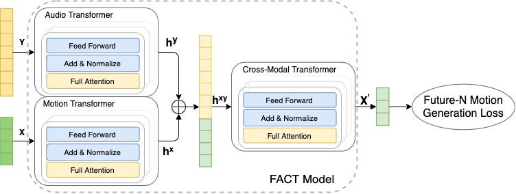
The FACT network takes in a music piece (Y) and a 2-second sequence of seed motion (X), then generates long-range future motions that correlate with the input music.

FACT involves three key design choices that are critical for producing realistic 3D dance motion from music.

All of the transformers use a full-attention mask, which can be more expressive than typical causal models because internal tokens have access to all inputs.
We train the model to predict N futures beyond the current input, instead of just the next motion. This encourages the network to pay more attention to the temporal context, and helps prevent the model from motion freezing or diverging after a few generation steps.
We fuse the two embeddings (motion and audio) early and employ a deep 12-layer cross-modal transformer module, which is essential for training a model that actually pays attention to the input music.

Results
We evaluate the performance based on three metrics:

Motion Quality: We calculate the Frechet Inception Distance (FID) between the real dance motion sequences in the AIST++ test set and 40 model generated motion sequences, each with 1200 frames (20 secs). We denote the FID based on the geometric and kinetic features as FID_g and FID_k, respectively.

Generation Diversity: Similar to prior work, to evaluate the model’s ability to generate divers dance motions, we calculate the average Euclidean distance in the feature space across 40 generated motions on the AIST++ test set, again comparing geometric feature space (Dist_g) and in the kinetic feature space (Dist_k).

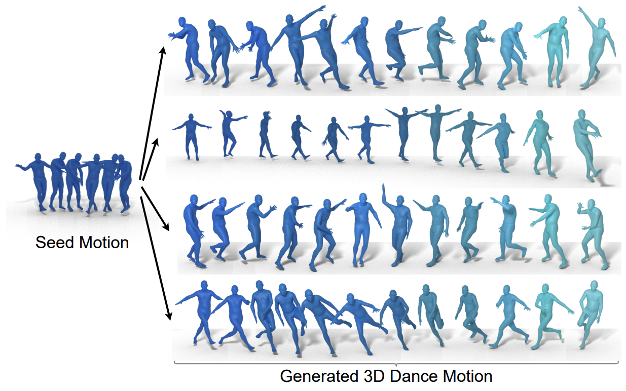
Four different dance choreographies (right) generated using different music, but the same two second seed motion (left). The genres of the conditioning music are: Break, Ballet Jazz, Krump and Middle Hip-hop. The seed motion comes from hip-hop dance.

Motion-Music Correlation: Because there is no well-designed metric to measure the correlation between input music (music beats) and generated 3D motion (kinematic beats), we propose a novel metric, called Beat Alignment Score (BeatAlign).

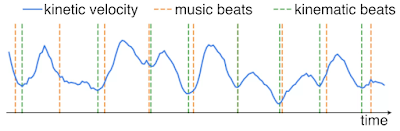
Kinetic velocity (blue curve) and kinematic beats (green dotted line) of the generated dance motion, as well as the music beats (orange dotted line). The kinematic beats are extracted by finding local minima from the kinetic velocity curve.

Quantitative Evaluation
We compare the performance of FACT on each of these metrics to that of other state-of-the-art methods.

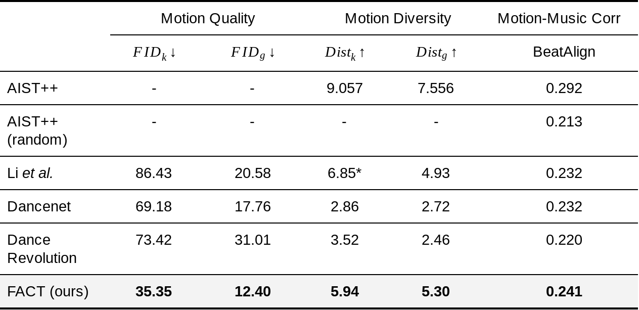
Compared to three recent state-of-the-art methods (Li et al., Dancenet, and Dance Revolution), the FACT model generates motions that are more realistic, better correlated with input music, and more diversified when conditioned on different music. *Note that the Li et al. generated motions are discontinuous, making the average kinetic feature distance abnormally high.

We also perceptually evaluate the motion-music correlation with a user study in which each participant is asked to watch 10 videos showing one of our results and one random counterpart, and then select which dancer is more in sync with the music. The study consisted of 30 participants, ranging from professional dancers to people who rarely dance. Compared to each baseline, 81% prefered the FACT model output to that of Li et al., 71% prefered FACT to Dancenet, and 77% prefered it Dance Revolution. Interestingly, 75% of participants preferred the unpaired AIST++ dance motion to that generated by FACT, which is unsurprising since the original dance captures are highly expressive.

Qualitative Results
Compared with prior methods like DanceNet (left) and Li et. al. (middle), 3D dance generated using the FACT model (right) is more realistic and better correlated with input music.

More generated 3D dances using the FACT model.

Conclusion and Discussion
We present a model that can not only learn the audio-motion correspondence, but also can generate high quality 3D motion sequences conditioned on music. Because generating 3D movement from music is a nascent area of study, we hope our work will pave the way for future cross-modal audio to 3D motion generation. We are also releasing AIST++, the largest 3D human dance dataset to date. This proposed, multi-view, multi-genre, cross-modal 3D motion dataset can not only help research in the conditional 3D motion generation research but also human understanding research in general. We are releasing the code in our GitHub repository and the trained model here.

While our results show a promising direction in this problem of music conditioned 3D motion generation, there are more to be explored. First, our approach is kinematic-based and we do not reason about physical interactions between the dancer and the floor. Therefore the global translation can lead to artifacts, such as foot sliding and floating. Second, our model is currently deterministic. Exploring how to generate multiple realistic dances per music is an exciting direction.

Acknowledgements
We gratefully acknowledge the contribution of other co-authors, including Ruilong Li and David Ross. We thank Chen Sun, Austin Myers, Bryan Seybold and Abhijit Kundu for helpful discussions. We thank Emre Aksan and Jiaman Li for sharing their code. We also thank Kevin Murphy for the early attempts in this direction, as well as Peggy Chi and Pan Chen for the help on user study experiments.

Source: Google AI Blog

Pixel Buds A-Series: Rich sound with an iconic design

When we first introduced our truly wireless Pixel Buds, we aimed to pack plenty of functionality into a surprisingly small product. Now, we’re making that same premium sound quality, along with hands-free help from Google Assistant and real-time translation.

Introducing Pixel Buds A-Series: rich sound, clear calls and Google helpfulness, all in a low-profile design, for ₹ 9,999.

A premium audio experience

Our research shows that most people describe great sound as full, clear and natural. This is what guides our audio tuning process and shows up in other devices, like Nest Audio. And Pixel Buds A-Series are no exception. Custom-designed 12 mm dynamic speaker drivers deliver full, clear and natural sound, with the option for even more power in those low tones with Bass Boost.

To experience the full range of the speaker’s capabilities, especially in the low frequencies, a good seal is essential. We’ve scanned thousands of ears to make Pixel Buds A-Series fit securely with a gentle seal. In order to keep the fit comfortable over time, a spatial vent reduces in-ear pressure.

Each earbud also connects to the main device playing audio, and has strong individual transmission power, to keep your sound clear and uninterrupted.

The stabilizer arc ensures a gentle, but secure fit while spatial vents prevent that plugged ear feeling.

Sound quality can also be affected by your environment. The new Pixel Buds A-Series come with Adaptive Sound, which increases or decreases the volume based on your surroundings. This comes in handy when you're moving from the quiet of your home to somewhere noisy like a city street, or while jogging past a loud construction site.

And your calls will have great sound, too. To make sure your calls are as clear as they can be, Pixel Buds A-Series use beamforming mics to focus on your voice and reduce outside noise, making your calls crystal clear (though of course, overall call quality depends on signal strength, environment, network, and other factors). Once your call is over, quickly get back to your music with a simple “Ok Google, play my music.”

Stylish and hardworking

For Pixel Buds A-Series, we wanted to bring back the iconic Clearly White, but added a twist with new gray undertones. We use nature for inspiration in our colors all the time, and our design team was looking to create soothing tones that evoke a sense of comfort and relaxation.

Pixel Buds’ design is inspired by the idea that great things can come in small packages: Pixel Buds A-Series include up to five hours of listening time on a single charge or up to 24 hours using the charging case. And with the ability to get a quick charge — about 15 minutes in the case gives you up to three hours of listening time — you can keep listening anywhere.1

They’re comfortable enough for those long listening sessions, and don’t worry if some of that time is devoted to a sweaty workout or a run in the rain: The earbuds are also sweat and water-resistant.2

Hands-free access to the best of Google

Google Assistant is built right into the Pixel Buds A-Series. You can get quick hands-free help to check the weather, get an answer, change the volume, or have notifications read to you with a simple “Ok Google.”

You can do more than just ask questions, though — for example, you can get real-time translation in more than 40 languages (including Bengali, Hindi, and Tamil) right in your ear while using a Pixel or Android 6.0+ phone. Say “Ok Google, help me speak French” to start a conversation. For more information, including available languages and minimum requirements, visit g.co/pixelbuds/help.

Pixel Buds A-Series work with any phone running bluetooth as standard wireless earbuds, delivering a quality listening experience. Features like the Google Assistant, Fast Pair, Find my Device, Adaptive Sound, and more work on all Pixel and Android devices running Android 6.0+.

Pixel Buds A-Series will be available for purchase on 25th August 2021 at Flipkart, Reliance Digital, and Tata Cliq, and will be coming to more retail outlets subsequently.

Posted by Austine Chang, Product Manager

1. All listening times are approximate and were measured using music playback with pre-production hardware and software, with fully charged Pixel Buds A-Series and case, and other features disabled. Case is used to recharge Pixel Buds A-Series when their batteries are depleted. Charging times are approximate. Use of other features will decrease battery life. Battery life depends on device, features enabled, usage, environment and many other factors. Actual battery life may be lower.

2. Pixel Buds A-Series (earbuds only) have a water protection rating of IPx4 under IEC standard 60529. Water resistance is not a permanent condition and may be compromised by normal wear and tear, repair, disassembly, or damage.

Source: Official Google India Blog

SoundStream: An End-to-End Neural Audio Codec

Posted by Neil Zeghidour, Research Scientist and Marco Tagliasacchi, Staff Research Scientist, Google Research

Audio codecs are used to efficiently compress audio to reduce either storage requirements or network bandwidth. Ideally, audio codecs should be transparent to the end user, so that the decoded audio is perceptually indistinguishable from the original and the encoding/decoding process does not introduce perceivable latency.

Over the past few years, different audio codecs have been successfully developed to meet these requirements, including Opus and Enhanced Voice Services (EVS). Opus is a versatile speech and audio codec, supporting bitrates from 6 kbps (kilobits per second) to 510 kbps, which has been widely deployed across applications ranging from video conferencing platforms, like Google Meet, to streaming services, like YouTube. EVS is the latest codec developed by the 3GPP standardization body targeting mobile telephony. Like Opus, it is a versatile codec operating at multiple bitrates, 5.9 kbps to 128 kbps. The quality of the reconstructed audio using either of these codecs is excellent at medium-to-low bitrates (12–20 kbps), but it degrades sharply when operating at very low bitrates (⪅3 kbps). While these codecs leverage expert knowledge of human perception as well as carefully engineered signal processing pipelines to maximize the efficiency of the compression algorithms, there has been recent interest in replacing these handcrafted pipelines by machine learning approaches that learn to encode audio in a data-driven manner.

Earlier this year, we released Lyra, a neural audio codec for low-bitrate speech. In “SoundStream: an End-to-End Neural Audio Codec”, we introduce a novel neural audio codec that extends those efforts by providing higher-quality audio and expanding to encode different sound types, including clean speech, noisy and reverberant speech, music, and environmental sounds. SoundStream is the first neural network codec to work on speech and music, while being able to run in real-time on a smartphone CPU. It is able to deliver state-of-the-art quality over a broad range of bitrates with a single trained model, which represents a significant advance in learnable codecs.

Learning an Audio Codec from Data
The main technical ingredient of SoundStream is a neural network, consisting of an encoder, decoder and quantizer, all of which are trained end-to-end. The encoder converts the input audio stream into a coded signal, which is compressed using the quantizer and then converted back to audio using the decoder. SoundStream leverages state-of-the-art solutions in the field of neural audio synthesis to deliver audio at high perceptual quality, by training a discriminator that computes a combination of adversarial and reconstruction loss functions that induce the reconstructed audio to sound like the uncompressed original input. Once trained, the encoder and decoder can be run on separate clients to efficiently transmit high-quality audio over a network.

SoundStream training and inference. During training, the encoder, quantizer and decoder parameters are optimized using a combination of reconstruction and adversarial losses, computed by a discriminator, which is trained to distinguish between the original input audio and the reconstructed audio. During inference, the encoder and quantizer on a transmitter client send the compressed bitstream to a receiver client that can then decode the audio signal.

Learning a Scalable Codec with Residual Vector Quantization
The encoder of SoundStream produces vectors that can take an indefinite number of values. In order to transmit them to the receiver using a limited number of bits, it is necessary to replace them by close vectors from a finite set (called a codebook), a process known as vector quantization. This approach works well at bitrates around 1 kbps or lower, but quickly reaches its limits when using higher bitrates. For example, even at a bitrate as low as 3 kbps, and assuming the encoder produces 100 vectors per second, one would need to store a codebook with more than 1 billion vectors, which is infeasible in practice.

In SoundStream, we address this issue by proposing a new residual vector quantizer (RVQ), consisting of several layers (up to 80 in our experiments). The first layer quantizes the code vectors with moderate resolution, and each of the following layers processes the residual error from the previous one. By splitting the quantization process in several layers, the codebook size can be reduced drastically. As an example, with 100 vectors per second at 3 kbps, and using 5 quantizer layers, the codebook size goes from 1 billion to 320. Moreover, we can easily increase or decrease the bitrate by adding or removing quantizer layers, respectively.

Because network conditions can vary while transmitting audio, ideally a codec should be “scalable” so that it can change its bitrate from low to high depending on the state of the network. While most traditional codecs are scalable, previous learnable codecs need to be trained and deployed specifically for each bitrate.

To circumvent this limitation, we leverage the fact that the number of quantization layers in SoundStream controls the bitrate, and propose a new method called “quantizer dropout”. During training, we randomly drop some quantization layers to simulate a varying bitrate. This pushes the decoder to perform well at any bitrate of the incoming audio stream, and thus helps SoundStream to become “scalable” so that a single trained model can operate at any bitrate, performing as well as models trained specifically for these bitrates.

Comparison of SoundStream models (higher is better) that are trained at 18 kbps with quantizer dropout (bitrate scalable), without quantizer dropout (not bitrate scalable) and evaluated with a variable number of quantizers, or trained and evaluated at a fixed bitrate (bitrate specific). The bitrate-scalable model (a single model for all bitrates) does not lose any quality when compared to bitrate-specific models (a different model for each bitrate), thanks to quantizer dropout.

A State-of-the-Art Audio Codec
SoundStream at 3 kbps outperforms Opus at 12 kbps and approaches the quality of EVS at 9.6 kbps, while using 3.2x–4x fewer bits. This means that encoding audio with SoundStream can provide a similar quality while using a significantly lower amount of bandwidth. Moreover, at the same bitrate, SoundStream outperforms the current version of Lyra, which is based on an autoregressive network. Unlike Lyra, which is already deployed and optimized for production usage, SoundStream is still at an experimental stage. In the future, Lyra will incorporate the components of SoundStream to provide both higher audio quality and reduced complexity.

SoundStream at 3kbps vs. state-of-the-art codecs. MUSHRA score is an indication of subjective quality (the higher the better).

The demonstration of SoundStream’s performance compared to Opus, EVS, and the original Lyra codec is presented in these audio examples, a selection of which are provided below.

Speech

Reference
Lyra (3kbps)
Opus (6kbps)
EVS (5.9kbps)
SoundStream (3kbps)

Music

Reference
Lyra (3kbps)
Opus (6kbps)
EVS (5.9kbps)
SoundStream (3kbps)

Joint Audio Compression and Enhancement
In traditional audio processing pipelines, compression and enhancement (the removal of background noise) are typically performed by different modules. For example, it is possible to apply an audio enhancement algorithm at the transmitter side, before audio is compressed, or at the receiver side, after audio is decoded. In such a setup, each processing step contributes to the end-to-end latency. Conversely, we design SoundStream in such a way that compression and enhancement can be carried out jointly by the same model, without increasing the overall latency. In the following examples, we show that it is possible to combine compression with background noise suppression, by activating and deactivating denoising dynamically (no denoising for 5 seconds, denoising for 5 seconds, no denoising for 5 seconds, etc.).

Original noisy audio
Denoised output*

* Demonstrated by turning denoising on and off every 5 seconds.

Conclusion
Efficient compression is necessary whenever one needs to transmit audio, whether when streaming a video, or during a conference call. SoundStream is an important step towards improving machine learning-driven audio codecs. It outperforms state-of-the-art codecs, such as Opus and EVS, can enhance audio on demand, and requires deployment of only a single scalable model, rather than many.

SoundStream will be released as a part of the next, improved version of Lyra. By integrating SoundStream with Lyra, developers can leverage the existing Lyra APIs and tools for their work, providing both flexibility and better sound quality. We will also release it as a separate TensorFlow model for experimentation.

AcknowledgmentsThe work described here was authored by Neil Zeghidour, Alejandro Luebs, Ahmed Omran, Jan Skoglund and Marco Tagliasacchi. We are grateful for all discussions and feedback on this work that we received from our colleagues at Google.

Source: Google AI Blog

Applying Advanced Speech Enhancement in Cochlear Implants

Posted by Samuel J. Yang, Research Scientist and Dick Lyon, Principal Scientist, Google Research

For the ~466 million people in the world who are deaf or hard of hearing, the lack of easy access to accessibility services can be a barrier to participating in spoken conversations encountered daily. While hearing aids can help alleviate this, simply amplifying sound is insufficient for many. One additional option that may be available is the cochlear implant (CI), which is an electronic device that is surgically inserted into a part of the inner ear, called the cochlea, and stimulates the auditory nerve electrically via external sound processors. While many individuals with these cochlear implants can learn to interpret these electrical stimulations as audible speech, the listening experience can be quite varied and particularly challenging in noisy environments.

Modern cochlear implants drive electrodes with pulsatile signals (i.e., discrete stimulation pulses) that are computed by external sound processors. The main challenge still facing the CI field is how to best process sounds — to convert sounds to pulses on electrodes — in a way that makes them more intelligible to users. Recently, to stimulate progress on this problem, scientists in industry and academia organized a CI Hackathon to open the problem up to a wider range of ideas.

In this post, we share exploratory research demonstrating that a speech enhancement preprocessor — specifically, a noise suppressor — can be used at the input of a CI’s processor to enhance users’ understanding of speech in noisy environments. We also discuss how we built on this work in our entry for the CI Hackathon and how we will continue developing this work.

Improving CIs with Noise Suppression
In 2019, a small internal project demonstrated the benefits of noise suppression at the input of a CI’s processor. In this project, participants listened to 60 pre-recorded and pre-processed audio samples and ranked them by their listening comfort. CI users listened to the audio using their devices' existing strategy for generating electrical pulses.

Audio without background noise


Audio with background noise


Audio with background noise + noise suppression

Background audio clip from “IMG_0991.MOV” by Kenny MacCarthy, license: CC-BY 2.0.

As shown below, both listening comfort and intelligibility usually increased, sometimes dramatically, when speech with noise (the lightest bar) was processed with noise suppression.

CI users in an early research study have improved listening comfort — qualitatively scored from "very poor" (0.0) to "OK" (0.5) to "very good" (1.0) — and speech intelligibility (i.e., the fraction of words in a sentence correctly transcribed) when trying to listen to noisy audio samples of speech with noise suppression applied.

For the CI Hackathon, we built on the project above, continuing to leverage our use of a noise suppressor while additionally exploring an approach to compute the pulses too

Overview of the Processing Approach
The hackathon considered a CI with 16 electrodes. Our approach decomposes the audio into 16 overlapping frequency bands, corresponding to the positions of the electrodes in the cochlea. Next, because the dynamic range of sound easily spans multiple orders of magnitude more than what we expect the electrodes to represent, we aggressively compress the dynamic range of the signal by applying "per-channel energy normalization" (PCEN). Finally, the range-compressed signals are used to create the electrodogram (i.e., what the CI displays on the electrodes).

In addition, the hackathon required a submission be evaluated in multiple audio categories, including music, which is an important but notoriously difficult category of sounds for CI users to enjoy. However, the speech enhancement network was trained to suppress non-speech sounds, including both noise and music, so we needed to take extra measures to avoid suppressing instrumental music (note that in general, music suppression might be preferred by some users in certain contexts). To do this, we created a “mix” of the original audio with the noise-suppressed audio so that enough of the music would pass through to remain audible. We varied in real-time the fraction of original audio mixed from 0% to 40% (0% if all of the input is estimated as speech, up to 40% as more of the input is estimated as non-speech) based on the estimate from the open-source YAMNet classifier on every ~1 second window of audio of whether the input is speech or non-speech.

The Conv-TasNet Speech Enhancement Model
To implement a speech enhancement module that suppresses non-speech sounds, such as noise and music, we use the Conv-TasNet model, which can separate different kinds of sounds. To start, the raw audio waveforms are transformed and processed into a form that can be used by a neural network. The model transforms short, 2.5 millisecond frames of input audio with a learnable analysis transform to generate features optimized for sound separation. The network then produces two “masks” from those features: one mask for speech and one mask for noise. These masks indicate the degree to which each feature corresponds to either speech or noise. Separated speech and noise are reconstructed back to the audio domain by multiplying the masks with the analysis features, applying a synthesis transform back to audio-domain frames, and stitching the resulting short frames together. As a final step, the speech and noise estimates are processed by a mixture consistency layer, which improves the quality of the estimated waveforms by ensuring that they sum up to the original input mixture waveform.

Block diagram of the speech enhancement system, which is based on Conv-TasNet.

The model is both causal and low latency: for each 2.5 milliseconds of input audio, the model produces estimates of separated speech and noise, and thus could be used in real-time. For the hackathon, to demonstrate what could be possible with increased compute power in future hardware, we chose to use a model variant with 2.9 million parameters. This model size is too large to be practically implemented in a CI today, but demonstrates what kind of performance would be possible with more capable hardware in the future.

Listening to the Results
As we optimized our models and overall solution, we used the hackathon-provided vocoder (which required a fixed temporal spacing of electrical pulses) to produce audio simulating what CI users might perceive. We then conducted blind A-B listening tests as typical hearing users.

Listening to the vocoder simulations below, the speech in the reconstructed sounds — from the vocoder processing the electrodograms — is reasonably intelligible when the input sound doesn't contain too much background noise, however there is still room to improve the clarity of the speech. Our submission performed well in the speech-in-noise category and achieved second place overall.

Simulated audio with fixed temporal spacing

Vocoder simulation of what CI users might perceive from audio from an electrodogram with fixed temporal spacing, with background noise and noise suppression applied.

A bottleneck on quality is that the fixed temporal spacing of stimulation pulses sacrifices fine-time structure in the audio. A change to the processing to produce pulses timed to peaks in the filtered sound waveforms captures more information about the pitch and structure of sound than is conventionally represented in implant stimulation patterns.

Simulated audio with adaptive spacing and fine time structure

Vocoder simulation, using the same vocoder as above, but on an electrodogram from the modified processing that synchronizes stimulation pulses to peaks of the sound waveform.

It's important to note that this second vocoder output is overly optimistic about how well it might sound to a real CI user. For instance, the simple vocoder used here does not model how current spread in the cochlea blurs the stimulus, making it harder to resolve different frequencies. But this at least suggests that preserving fine-time structure is valuable and that the electrodogram itself is not the bottleneck.

Ideally, all processing approaches would be evaluated by a broad range of CI users, with the electrodograms implemented directly on their CIs rather than relying upon vocoder simulations.

Conclusion and a Call to Collaborate
We are planning to follow up on this experience in two main directions. First, we plan to explore the application of noise suppression to other hearing-accessibility modalities, including hearing aids, transcription, and vibrotactile sensory substitution. Second, we'll take a deeper dive into the creation of electrodogram patterns for cochlear implants, exploiting fine temporal structure that is not accommodated in the usual CIS (continous interleaved sampling) patterns that are standard in the industry. According to Louizou: “It remains a puzzle how some single-channel patients can perform so well given the limited spectral information they receive''. Therefore, using fine temporal structure might be a critical step towards achieving an improved CI experience.

Google is committed to building technology with and for people with disabilities. If you are interested in collaborating to improve the state of the art in cochlear implants (or hearing aids), please reach out to [email protected].

Acknowledgements
We would like to thank the Cochlear Impact hackathon organizers for giving us this opportunity and partnering with us. The participating team within Google is Samuel J. Yang, Scott Wisdom, Pascal Getreuer, Chet Gnegy, Mihajlo Velimirović, Sagar Savla, and Richard F. Lyon with guidance from Dan Ellis and Manoj Plakal.

Source: Google AI Blog

Applying Advanced Speech Enhancement in Cochlear Implants

Posted by Samuel J. Yang, Research Scientist and Dick Lyon, Principal Scientist, Google Research

Audio without background noise


Audio with background noise


Audio with background noise + noise suppression

Background audio clip from “IMG_0991.MOV” by Kenny MacCarthy, license: CC-BY 2.0.

As shown below, both listening comfort and intelligibility usually increased, sometimes dramatically, when speech with noise (the lightest bar) was processed with noise suppression.

For the CI Hackathon, we built on the project above, continuing to leverage our use of a noise suppressor while additionally exploring an approach to compute the pulses too

Block diagram of the speech enhancement system, which is based on Conv-TasNet.

Simulated audio with fixed temporal spacing

Vocoder simulation of what CI users might perceive from audio from an electrodogram with fixed temporal spacing, with background noise and noise suppression applied.

Simulated audio with adaptive spacing and fine time structure

Vocoder simulation, using the same vocoder as above, but on an electrodogram from the modified processing that synchronizes stimulation pulses to peaks of the sound waveform.

Ideally, all processing approaches would be evaluated by a broad range of CI users, with the electrodograms implemented directly on their CIs rather than relying upon vocoder simulations.

Source: Google AI Blog

Lyra – enabling voice calls for the next billion users

The past year has shown just how vital online communication is to our lives. Never before has it been more important to clearly understand one another online, regardless of where you are and whatever network conditions are available. That’s why in February we introduced Lyra: a revolutionary new audio codec using machine learning to produce high-quality voice calls.

As part of our efforts to make the best codecs universally available, we are open sourcing Lyra, allowing other developers to power their communications apps and take Lyra in powerful new directions. This release provides the tools needed for developers to encode and decode audio with Lyra, optimized for the 64-bit ARM android platform, with development on Linux. We hope to expand this codebase and develop improvements and support for additional platforms in tandem with the community.

The Lyra Architecture

Lyra’s architecture is separated into two pieces, the encoder and decoder. When someone talks into their phone the encoder captures distinctive attributes from their speech. These speech attributes, also called features, are extracted in chunks of 40ms, then compressed and sent over the network. It is the decoder’s job to convert the features back into an audio waveform that can be played out over the listener’s phone speaker. The features are decoded back into a waveform via a generative model. Generative models are a particular type of machine learning model well suited to recreate a full audio waveform from a limited number of features. The Lyra architecture is very similar to traditional audio codecs, which have formed the backbone of internet communication for decades. Whereas these traditional codecs are based on digital signal processing (DSP) techniques, the key advantage for Lyra comes from the ability of the generative model to reconstruct a high-quality voice signal.

The Impact

While mobile connectivity has steadily increased over the past decade, the explosive growth of on-device compute power has outstripped access to reliable high speed wireless infrastructure. For regions where this contrast exists—in particular developing countries where the next billion internet users are coming online—the promise that technology will enable people to be more connected has remained elusive. Even in areas with highly reliable connections, the emergence of work-from-anywhere and telecommuting have further strained mobile data limits. While Lyra compresses raw audio down to 3kbps for quality that compares favourably to other codecs, such as Opus, it is not aiming to be a complete alternative, but can save meaningful bandwidth in these kinds of scenarios.

These trends provided motivation for Lyra and are the reason our open source library focuses on its potential for real time voice communication. There are also other applications we recognize Lyra may be uniquely well suited for, from archiving large amounts of speech, and saving battery by leveraging the computationally cheap Lyra encoder, to alleviating network congestion in emergency situations where many people are trying to make calls at once. We are excited to see the creativity the open source community is known for applied to Lyra in order to come up with even more unique and impactful applications.

The Open Source Release

The Lyra code is written in C++ for speed, efficiency, and interoperability, using the Bazel build framework with Abseil and the GoogleTest framework for thorough unit testing. The core API provides an interface for encoding and decoding at the file and packet levels. The complete signal processing toolchain is also provided, which includes various filters and transforms. Our example app integrates with the Android NDK to show how to integrate the native Lyra code into a Java-based android app. We also provide the weights and vector quantizers that are necessary to run Lyra.

We are releasing Lyra as a beta version today because we wanted to enable developers and get feedback as soon as possible. As a result, we expect the API and bitstream to change as it is developed. All of the code for running Lyra is open sourced under the Apache license, except for a math kernel, for which a shared library is provided until we can implement a fully open solution over more platforms. We look forward to seeing what people do with Lyra now that it is open sourced. Check out the code and demo on GitHub, let us know what you think, and how you plan to use it!

By Andrew Storus and Michael Chinen – Chrome

Acknowledgements

The following people helped make the open source release possible:
Yero Yeh, Alejandro Luebs, Jamieson Brettle, Tom Denton, Felicia Lim, Bastiaan Kleijn, Jan Skoglund, Yaowu Xu, Jim Bankoski (Chrome), Chenjie Gu, Zach Gleicher, Tom Walters, Norman Casagrande, Luis Cobo, Erich Elsen (DeepMind).