Tag Archives: machine learning

Machine Learning Communities: Q2 ‘22 highlights and achievements

Posted by Nari Yoon, Hee Jung, DevRel Community Manager / Soonson Kwon, DevRel Program Manager

Let’s explore highlights and accomplishments of vast Google Machine Learning communities over the second quarter of the year! We are enthusiastic and grateful about all the activities by the global network of ML communities. Here are the highlights!

TensorFlow/Keras

TFUG Agadir hosted #MLReady phase as a part of #30DaysOfML. #MLReady aimed to prepare the attendees with the knowledge required to understand the different types of problems which deep learning can solve, and helped attendees be prepared for the TensorFlow Certificate.

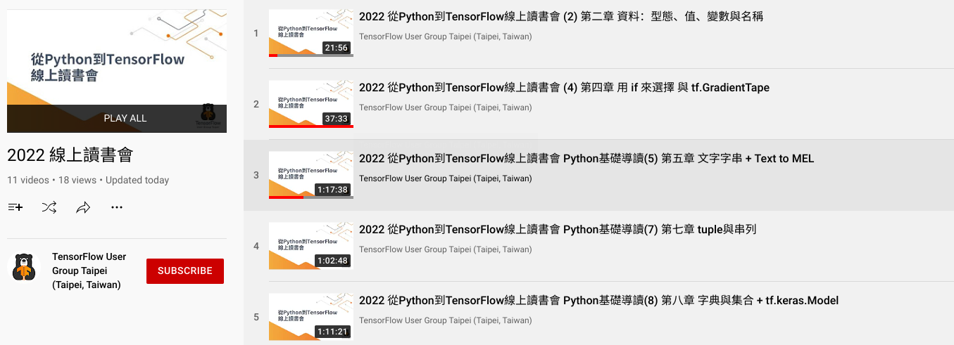
TFUG Taipei hosted the basic Python and TensorFlow courses named From Python to TensorFlow. The aim of these events is to help everyone learn about the basics of Python and TensorFlow, including TensorFlow Hub, TensorFlow API. The event videos are shared every week via Youtube playlist.

TFUG New York hosted Introduction to Neural Radiance Fields for TensorFlow users. The talk included Volume Rendering, 3D view synthesis, and links to a minimal implementation of NeRF using Keras and TensorFlow. In the event, ML GDE Aritra Roy Gosthipaty (India) had a talk focusing on breaking the concepts of the academic paper, NeRF: Representing Scenes as Neural Radiance Fields for View Synthesis into simpler and more ingestible snippets.

TFUG Turkey, GDG Edirne and GDG Mersin organized a TensorFlow Bootcamp 22 and ML GDE M. Yusuf Sarıgöz (Turkey) participated as a speaker, TensorFlow Ecosystem: Get most out of auxiliary packages. Yusuf demonstrated the inner workings of TensorFlow, how variables, tensors and operations interact with each other, and how auxiliary packages are built upon this skeleton.

TFUG Mumbai hosted the June Meetup and 110 folks gathered. ML GDE Sayak Paul (India) and TFUG mentor Darshan Despande shared knowledge through sessions. And ML workshops for beginners went on and participants built up machine learning models without writing a single line of code.

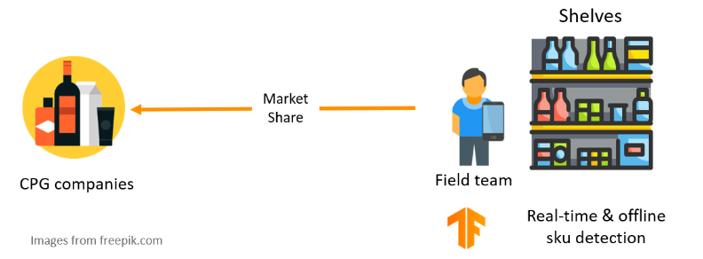
ML GDE Hugo Zanini (Brazil) wrote Realtime SKU detection in the browser using TensorFlow.js. He shared a solution for a well-known problem in the consumer packaged goods (CPG) industry: real-time and offline SKU detection using TensorFlow.js.

ML GDE Gad Benram (Portugal) wrote Can a couple TensorFlow lines reduce overfitting? He explained how just a few lines of code can generate data augmentations and boost a model’s performance on the validation set.

ML GDE Victor Dibia (USA) wrote How to Build An Android App and Integrate Tensorflow ML Models sharing how to run machine learning models locally on Android mobile devices, How to Implement Gradient Explanations for a HuggingFace Text Classification Model (Tensorflow 2.0) explaining in 5 steps about how to verify the model is focusing on the right tokens to classify text. He also wrote how to finetune a HuggingFace model for text classification, using Tensorflow 2.0.

ML GDE Karthic Rao (India) released a new series ML for JS developers with TFJS. This series is a combination of short portrait and long landscape videos. You can learn how to build a toxic word detector using TensorFlow.js.

ML GDE Sayak Paul (India) implemented the DeiT family of ViT models, ported the pre-trained params into the implementation, and provided code for off-the-shelf inference, fine-tuning, visualizing attention rollout plots, distilling ViT models through attention. (code | pretrained model | tutorial)

ML GDE Sayak Paul (India) and ML GDE Aritra Roy Gosthipaty (India) inspected various phenomena of a Vision Transformer, shared insights from various relevant works done in the area, and provided concise implementations that are compatible with Keras models. They provide tools to probe into the representations learned by different families of Vision Transformers. (tutorial | code)

JAX/Flax

ML GDE Aakash Nain (India) had a special talk, Introduction to JAX for ML GDEs, TFUG organizers and ML community network organizers. He covered the fundamentals of JAX/Flax so that more and more people try out JAX in the near future.

ML GDE Seunghyun Lee (Korea) started a project, Training and Lightweighting Cookbook in JAX/FLAX. This project attempts to build a neural network training and lightweighting cookbook including three kinds of lightweighting solutions, i.e., knowledge distillation, filter pruning, and quantization.

ML GDE Yucheng Wang (China) wrote History and features of JAX and explained the difference between JAX and Tensorflow.

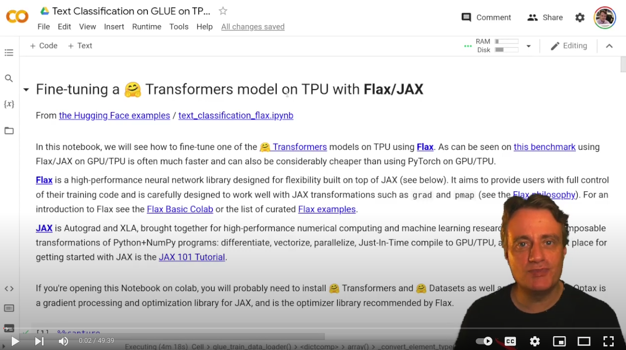
ML GDE Martin Andrews (Singapore) shared a video, Practical JAX : Using Hugging Face BERT on TPUs. He reviewed the Hugging Face BERT code, written in JAX/Flax, being fine-tuned on Google’s Colab using Google TPUs. (Notebook for the video)

ML GDE Soumik Rakshit (India) wrote Implementing NeRF in JAX. He attempts to create a minimal implementation of 3D volumetric rendering of scenes represented by Neural Radiance Fields.

Kaggle

ML GDEs’ Kaggle notebooks were announced as the winner of Google OSS Expert Prize on Kaggle: Sayak Paul and Aritra Roy Gosthipaty’s Masked Image Modeling with Autoencoders in March; Sayak Paul’s Distilling Vision Transformers in April; Sayak Paul & Aritra Roy Gosthipaty’s Investigating Vision Transformer Representations; Soumik Rakshit’s Tensorflow Implementation of Zero-Reference Deep Curve Estimation in May and Aakash Nain’s The Definitive Guide to Augmentation in TensorFlow and JAX in June.

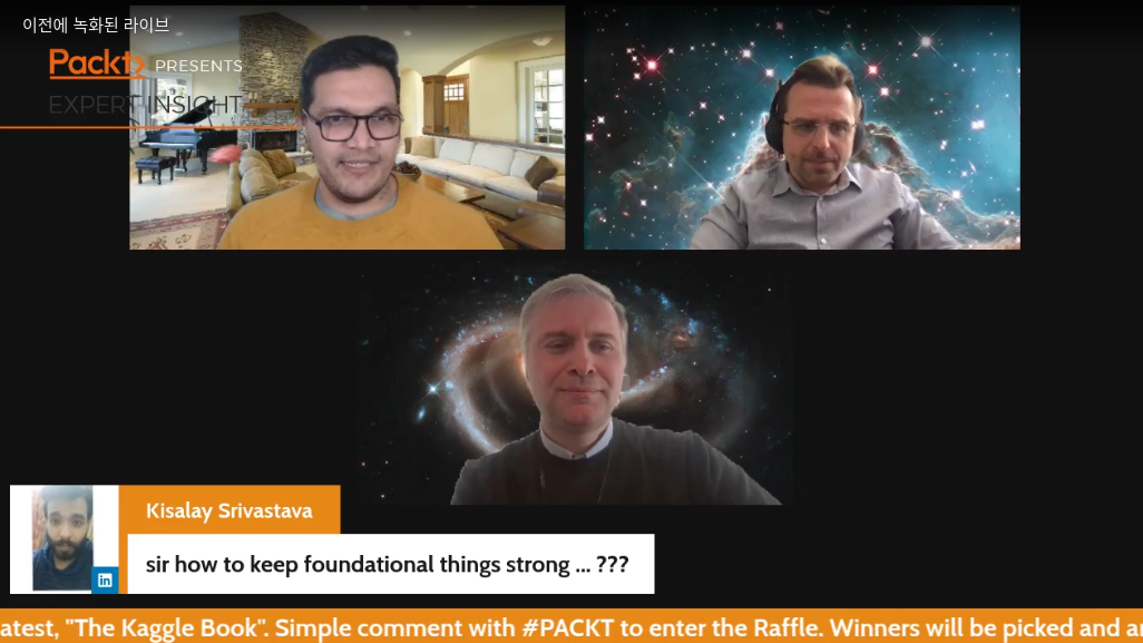
ML GDE Luca Massaron (Italy) published The Kaggle Book with Konrad Banachewicz. This book details competition analysis, sample code, end-to-end pipelines, best practices, and tips & tricks. And in the online event, Luca and the co-author talked about how to compete on Kaggle.


ML GDE Ertuğrul Demir (Turkey) wrote Kaggle Handbook: Fundamentals to Survive a Kaggle Shake-up covering bias-variance tradeoff, validation set, and cross validation approach. In the second post of the series, he showed more techniques using analogies and case studies.


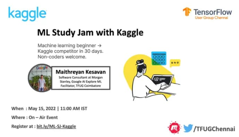
TFUG Chennai hosted ML Study Jam with Kaggle and created study groups for the interested participants. More than 60% of members were active during the whole program and many of them shared their completion certificates.

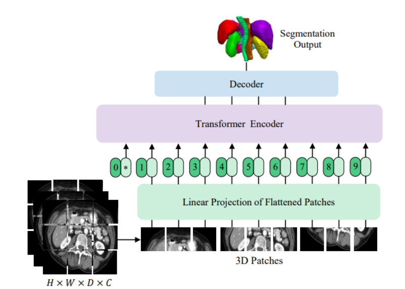
TFUG Mysuru organizer Usha Rengaraju shared a Kaggle notebook which contains the implementation of the research paper: UNETR - Transformers for 3D Biomedical Image Segmentation. The model automatically segments the stomach and intestines on MRI scans.

TFX

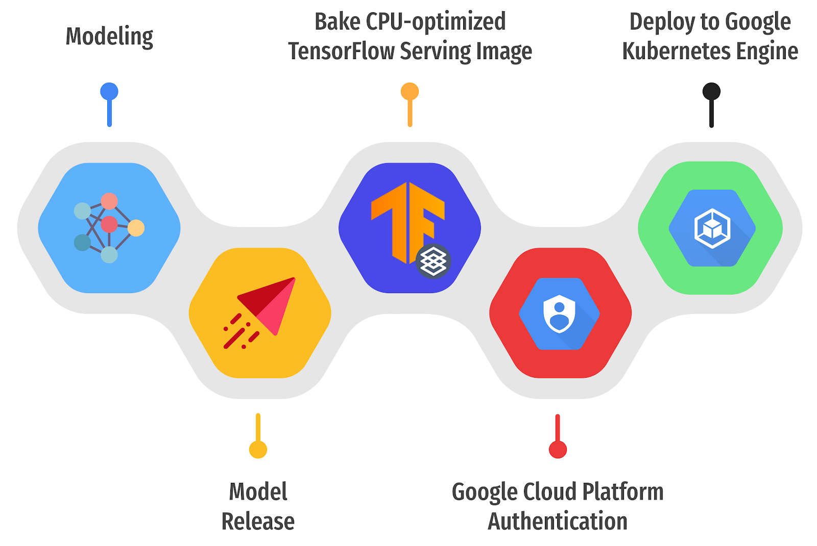
ML GDE Sayak Paul (India) and ML GDE Chansung Park (Korea) shared how to deploy a deep learning model with Docker, Kubernetes, and Github actions, with two promising ways - FastAPI (for REST) and TF Serving (for gRPC).

ML GDE Ukjae Jeong (Korea) and ML Engineers at Karrot Market, a mobile commerce unicorn with 23M users, wrote Why Karrot Uses TFX, and How to Improve Productivity on ML Pipeline Development.

ML GDE Jun Jiang (China) had a talk introducing the concept of MLOps, the production-level end-to-end solutions of Google & TensorFlow, and how to use TFX to build the search and recommendation system & scientific research platform for large-scale machine learning training.

ML GDE Piero Esposito (Brazil) wrote Building Deep Learning Pipelines with Tensorflow Extended. He showed how to get started with TFX locally and how to move a TFX pipeline from local environment to Vertex AI; and provided code samples to adapt and get started with TFX.

TFUG São Paulo (Brazil) had a series of online webinars on TensorFlow and TFX. In the TFX session, they focused on how to put the models into production. They talked about the data structures in TFX and implementation of the first pipeline in TFX: ingesting and validating data.

TFUG Stockholm hosted MLOps, TensorFlow in Production, and TFX covering why, what and how you can effectively leverage MLOps best practices to scale ML efforts and had a look at how TFX can be used for designing and deploying ML pipelines.

Cloud AI

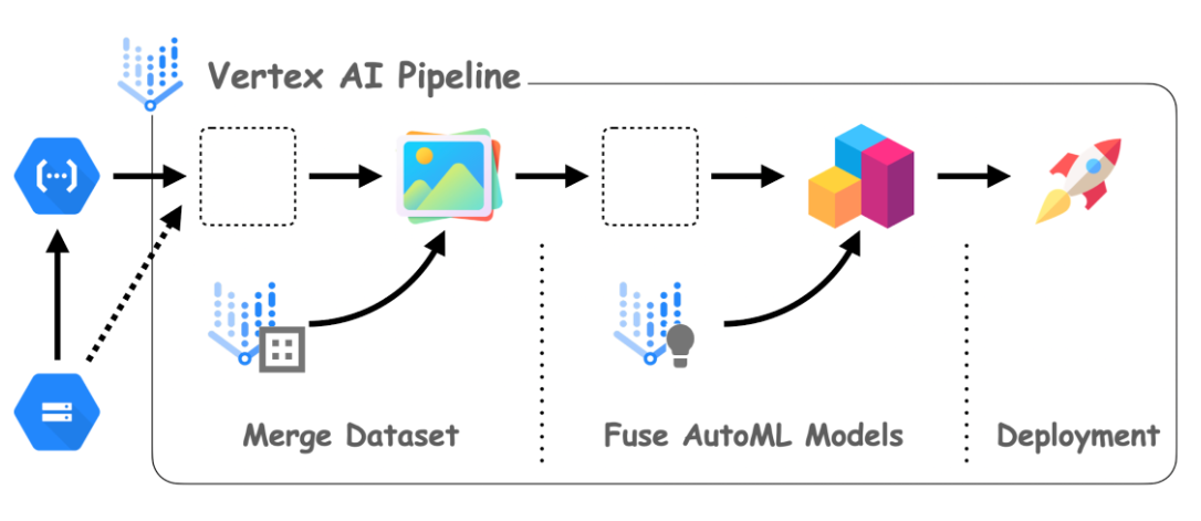
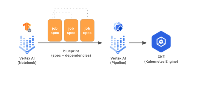
ML GDE Chansung Park (Korea) wrote MLOps System with AutoML and Pipeline in Vertex AI on GCP official blog. He showed how Google Cloud Storage and Google Cloud Functions can help manage data and handle events in the MLOps system.

He also shared the Github repository, Continuous Adaptation with VertexAI's AutoML and Pipeline. This contains two notebooks to demonstrate how to automate to produce a new AutoML model when the new dataset comes in.

TFUG Northwest (Portland) hosted The State and Future of AI + ML/MLOps/VertexAI lab walkthrough. In this event, ML GDE Al Kari (USA) outlined the technology landscape of AI, ML, MLOps and frameworks. Googler Andrew Ferlitsch had a talk about Google Cloud AI’s definition of the 8 stages of MLOps for enterprise scale production and how Vertex AI fits into each stage. And MLOps engineer Chris Thompson covered how easy it is to deploy a model using the Vertex AI tools.

Research

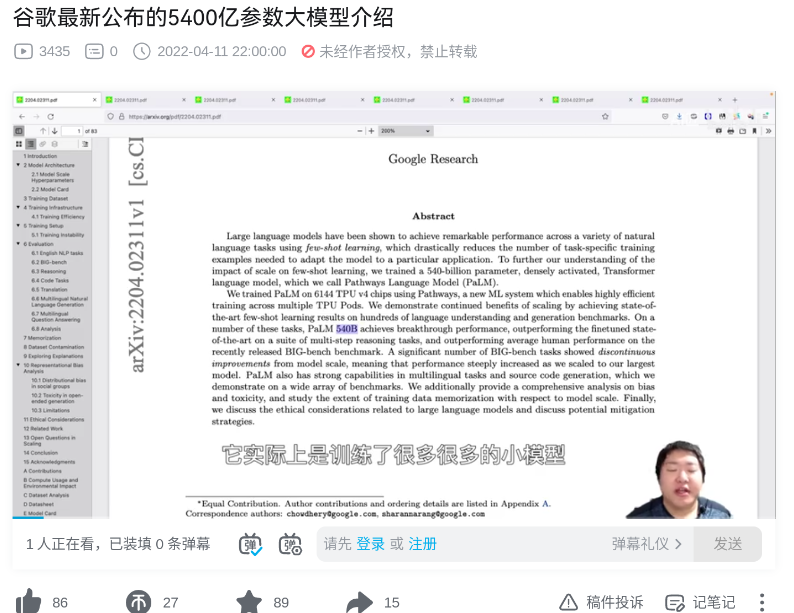
ML GDE Qinghua Duan (China) released a video which introduces Google’s latest 540 billion parameter model. He introduced the paper PaLM, and described the basic training process and innovations.

ML GDE Rumei LI (China) wrote blog postings reviewing papers, DeepMind's Flamingo and Google's PaLM.

Simplified Transfer Learning for Chest Radiography Model Development

Every year, nearly a billion chest X-ray (CXR) images are taken globally to aid in the detection and management of health conditions ranging from collapsed lungs to infectious diseases. Generally, CXRs are cheaper and more accessible than other forms of medical imaging. However, existing challenges continue to impede the optimal use of CXRs. For example, in some areas, trained radiologists that can accurately interpret CXR images are in short supply. In addition, interpretation variability between experts, workflow differences between institutions, and the presence of rare conditions familiar only to subspecialists all contribute to making high-quality CXR interpretation a challenge.

Recent research has leveraged machine learning (ML) to explore potential solutions for some of these challenges. There is significant interest and effort devoted to building deep learning models that detect abnormalities in CXRs and improve access, accuracy, and efficiency to identify diseases and conditions that affect the heart and lungs. However, building robust CXR models requires large labeled training datasets, which can be prohibitively expensive and time-consuming to create. In some cases, such as working with underrepresented populations or studying rare medical conditions, only limited data are available. Additionally, CXR images vary in quality across populations, geographies, and institutions, making it difficult to build robust models that perform well globally.

In “Simplified Transfer Learning for Chest Radiography Models Using Less Data”, published in the journal Radiology, we describe how Google Health utilizes advanced ML methods to generate pre-trained “CXR networks” that can convert CXR images to embeddings (i.e., information-rich numerical vectors) to enable the development of CXR models using less data and fewer computational resources. We demonstrate that even with less data and compute, this approach has enabled performance comparable to state-of-the-art deep learning models across various prediction tasks. We are also excited to announce the release of CXR Foundation, a tool that utilizes our CXR-specific network to enable developers to create custom embeddings for their CXR images. We believe this work will help accelerate the development of CXR models, aiding in disease detection and contributing to more equitable health access throughout the world.

Developing a Chest X-ray Network
A common approach to building medical ML models is to pre-train a model on a generic task using non-medical datasets and then refine the model on a target medical task. This process of transfer learning may improve the target task performance or at least speed up convergence by applying the understanding of natural images to medical images. However, transfer learning may still require large labeled medical datasets for the refinement step.

Expanding on this standard approach, our system supports modeling CXR-specific tasks through a three-step model training setup composed of (1) generic image pre-training similar to traditional transfer learning, (2) CXR-specific pre-training, and (3) task-specific training. The first and third steps are common in ML: first pre-training on a large dataset and labels that are not specific to the desired task, and then fine-tuning on the task of interest.

We built a CXR-specific image classifier that employs supervised contrastive learning (SupCon). SupCon pulls together representations of images that have the same label (e.g., abnormal) and pushes apart representations of images that have a different label (e.g., one normal image and one abnormal image). We pre-trained this model on de-identified CXR datasets of over 800,000 images generated in partnership with Northwestern Medicine and Apollo Hospitals in the US and India, respectively. We then leveraged noisy abnormality labels from natural language processing of radiology reports to build our “CXR-specific” network.

This network creates embeddings (i.e., information-rich numerical vectors that can be used to distinguish classes from each other) that can more easily train models for specific medical prediction tasks, such as image finding (e.g., airspace opacity), clinical condition (e.g., tuberculosis), or patient outcome (e.g., hospitalization). For example, the CXR network can generate embeddings for every image in a given CXR dataset. For these images, the generated embeddings and the labels for the desired target task (such as tuberculosis) are used as examples to train a small ML model.

Left: Training a CXR model for a given task generally requires a large number of labeled images and a significant amount of computational resources to create a foundation of neural network layers. Right: With the CXR network and tool providing this foundation, each new task requires only a fraction of the labeled images, computational resources, and neural network parameters compared to rebuilding the entire network from scratch.

Effects of CXR Pre-training
We visualized these embedding layers at each step of the process using airspace opacity as an example (see the figure below). Before SupCon-based pre-training, there was poor separation of normal and abnormal CXR embeddings. After SupCon-based pre-training, the positive examples were grouped more closely together, and the negative examples more closely together as well, indicating that the model had identified that images from each category resembled themselves.

Visualizations of the t-distributed stochastic neighbor embedding for generic vs. CXR-specific network embeddings. Embeddings are information-rich numerical vectors that alone can distinguish classes from each other, in this case, airspace opacity positive vs. negative.

Our research suggests that adding the second stage of pre-training enables high-quality models to be trained with up to 600-fold less data in comparison to traditional transfer learning approaches that leverage pre-trained models on generic, non-medical datasets. We found this to be true regardless of model architecture (e.g., ResNet or EfficientNet) or dataset used for natural image pre-training (e.g., ImageNet or JFT-300M). With this approach, researchers and developers can significantly reduce dataset size requirements.

Top: In a deep learning model, the neural network contains multiple layers of artificial neurons, with the first layer taking the CXR image as input, intermediate layers doing additional computation, and the final layer making the classification (e.g., airspace opacity: present vs. absent). The embedding layer is usually one of the last layers. Bottom left: The traditional transfer learning approach involves a two-step training setup where a generic pre-trained network is optimized directly on a prediction task of interest. Our proposed three-step training setup generates a CXR network using a SupCon ML technique (step 2) before optimization for prediction tasks of interest (step 3). Bottom right: Using the embeddings involves either training smaller models (the first two strategies) or fine-tuning the whole network if there are sufficient data (strategy 3).

Results
After training the initial model, we measured performance using the area under the curve (AUC) metric with both linear and non-linear models applied to CXR embeddings; and a non-linear model produced by fine-tuning the entire network. On public datasets, such as ChestX-ray14 and CheXpert, our work substantially and consistently improved the data-accuracy tradeoff for models developed across a range of training dataset sizes and several findings. For example, when evaluating the tool’s ability to develop tuberculosis models, data efficiency gains were more striking: models trained on the embeddings of just 45 images achieved non-inferiority to radiologists in detecting tuberculosis on an external validation dataset. For both tuberculosis and severe COVID-19 outcomes, we show that non-linear classifiers trained on frozen embeddings outperformed a model that was fine-tuned on the entire dataset.

Comparing CXR-specific networks for transfer learning (red), with a baseline transfer learning approach (blue) across a variety of CXR abnormalities (top left), tuberculosis (bottom left), and COVID-19 outcomes (bottom right). This approach improves performance at the same dataset size, or reduces the dataset size required to reach the same performance. Interestingly, using the CXR network with simpler ML models that are faster to train (red) performs better than training the full network (black) at dataset sizes up to 85 images.

Conclusion and Future Work
To accelerate CXR modeling efforts with low data and computational requirements, we are releasing our CXR Foundation tool, along with scripts to train linear and nonlinear classifiers. Via these embeddings, this tool will allow researchers to jump-start CXR modeling efforts using simpler transfer learning methods. This approach can be particularly useful for predictive modeling using small datasets, and for adapting CXR models when there are distribution shifts in patient populations (whether over time or across different institutions). We are excited to continue working with partners, such as Northwestern Medicine and Apollo Hospitals, to explore the impact of this technology further. By enabling researchers with limited data and compute to develop CXR models, we're hoping more developers can solve the most impactful problems for their populations.

Acknowledgements
Key contributors to this project at Google include Christina Chen, Yun Liu, Dilip Krishnan, Zaid Nabulsi, Atilla Kiraly, Arnav Agharwal, Eric Wu, Yuanzhen Li, Aaron Maschinot, Aaron Sarna, Jenny Huang, Marilyn Zhang, Charles Lau, Neeral Beladia, Daniel Tse, Krish Eswaran, and Shravya Shetty. Significant contributions and input were also made by collaborators Sreenivasa Raju Kalidindi, Mozziyar Etemadi, Florencia Garcia-Vicente, and David Melnick. For the ChestX-ray14 dataset, we thank the NIH Clinical Center for making it publicly available. The authors would also like to acknowledge many members of the Google Health Radiology and labeling software teams. Sincere appreciation also goes to the radiologists who enabled this work with their image interpretation and annotation efforts throughout the study; Jonny Wong for coordinating the imaging annotation work; Craig Mermel and Akinori Mitani for providing feedback on the manuscript; Nicole Linton and Lauren Winer for feedback on the blogpost; and Tom Small for the animation.

Source: Google AI Blog


Enabling Creative Expression with Concept Activation Vectors

Advances in computer vision and natural language processing continue to unlock new ways of exploring billions of images available on public and searchable websites. Today’s visual search tools make it possible to search with your camera, voice, text, images, or multiple modalities at the same time. However, it remains difficult to input subjective concepts, such as visual tones or moods, into current systems. For this reason, we have been working collaboratively with artists, photographers, and image researchers to explore how machine learning (ML) might enable people to use expressive queries as a way of visually exploring datasets.

Today, we are introducing Mood Board Search, a new ML-powered research tool that uses mood boards as a query over image collections. This enables people to define and evoke visual concepts on their own terms. Mood Board Search can be useful for subjective queries, such as “peaceful”, or for words and individual images that may not be specific enough to produce useful results in a standard search, such as “abstract details in overlooked scenes” or “vibrant color palette that feels part memory, part dream". We developed, and will continue to develop, this research tool in alignment with our AI Principles.

Search Using Mood Boards
With Mood Board Search, our goal is to design a flexible and approachable interface so people without ML expertise can train a computer to recognize a visual concept as they see it. The tool interface is inspired by mood boards, commonly used by people in creative fields to communicate the “feel” of an idea using collections of visual materials.

With Mood Board Search, users can train a computer to recognize visual concepts in image collections.

To get started, simply drag and drop a small number of images that represent the idea you want to convey. Mood Board Search returns the best results when the images share a consistent visual quality, so results are more likely to be relevant with mood boards that share visual similarities in color, pattern, texture, or composition.

It’s also possible to signal which images are more important to a visual concept by upweighting or downweighting images, or by adding images that are the opposite of the concept. Then, users can review and inspect search results to understand which part of an image best matches the visual concept. Focus mode does this by revealing a bounding box around part of the image, while AI crop cuts in directly, making it easier to draw attention to new compositions.

Supported interactions, like AI crop, allow users to see which part of an image best matches their visual concept.

Powered by Concept Activation Vectors (CAVs)
Mood Board Search takes advantage of pre-trained computer vision models, such as GoogLeNet and MobileNet, and a machine learning approach called Concept Activation Vectors (CAVs).

CAVs are a way for machines to represent images (what we understand) using numbers or directions in a neural net’s embedding space (which can be thought of as what machines understand). CAVs can be used as part of a technique, Testing with CAVs (TCAV), to quantify the degree to which a user-defined concept is important to a classification result; e.g., how sensitive a prediction of "zebra" is to the presence of stripes. This is a research approach we open-sourced in 2018, and the work has since been widely applied to medical applications and science to build ML applications that can provide better explanations for what machines see. You can learn more about embedding vectors in general in this Google AI blog post, and our approach to working with TCAVs in Been Kim’s Keynote at ICLR.

In Mood Board Search, we use CAVs to find a model's sensitivity to a mood board created by the user. In other words, each mood board creates a CAV — a direction in embedding space — and the tool searches an image dataset, surfacing images that are the closest match to the CAV. However, the tool takes it one step further, by segmenting each image in the dataset in 15 different ways, to uncover as many relevant compositions as possible. This is the approach behind features like Focus mode and AI crop.

Three artists created visual concepts to share their way of seeing, shown here in an experimental app by design invention studio, Nord Projects.

Because embedding vectors can be learned and re-used across models, tools like Mood Board Search can help us express our perspective to other people. Early collaborations with creative communities have shown value in being able to create and share subjective experiences with others, resulting in feelings of being able to “break out of visually-similar echo chambers” or “see the world through another person’s eyes”. Even misalignment between model and human understanding of a concept frequently resulted in unexpected and inspiring connections for collaborators. Taken together, these findings point towards new ways of designing collaborative ML systems that embrace personal and collective subjectivity.

Conclusions and Future Work
Today, we’re open-sourcing the code to Mood Board Search, including three visual concepts made by our collaborators, and a Mood Board Search Python Library for people to tap the power of CAVs directly into their own websites and apps. While these tools are early-stage prototypes, we believe this capability can have a wide-range of applications from exploring unorganized image collections to externalizing ways of seeing into collaborative and shareable artifacts. Already, an experimental app by design invention studio Nord Projects, made using Mood Board Search, investigates the opportunities for running CAVs in camera, in real-time. In future work, we plan to use Mood Board Search to learn about new forms of human-machine collaboration and expand ML models and inputs — like text and audio — to allow even deeper subjective discoveries, regardless of medium.

If you’re interested in a demo of this work for your team or organization, email us at [email protected].

Acknowledgments
This blog presents research by (in alphabetical order): Kira Awadalla, Been Kim, Eva Kozanecka, Alison Lentz, Alice Moloney, Emily Reif, and Oliver Siy, in collaboration with design invention studio Nord Projects. We thank our co-author, Eva Kozanecka, our artist collaborators, Alexander Etchells, Tom Hatton, Rachel Maggart, the Imaging team at The British Library for their participation in beta previews, and Blaise Agüera y Arcas, Jess Holbrook, Fernanda Viegas, and Martin Wattenberg for their support of this research project.

Source: Google AI Blog


MLGO: A Machine Learning Framework for Compiler Optimization

The question of how to compile faster and smaller code arose together with the birth of modem computers. Better code optimization can significantly reduce the operational cost of large datacenter applications. The size of compiled code matters the most to mobile and embedded systems or software deployed on secure boot partitions, where the compiled binary must fit in tight code size budgets. With advances in the field, the headroom has been heavily squeezed with increasingly complicated heuristics, impeding maintenance and further improvements.

Recent research has shown that machine learning (ML) can unlock more opportunities in compiler optimization by replacing complicated heuristics with ML policies. However, adopting ML in general-purpose, industry-strength compilers remains a challenge.

To address this, we introduce “MLGO: a Machine Learning Guided Compiler Optimizations Framework”, the first industrial-grade general framework for integrating ML techniques systematically in LLVM (an open-source industrial compiler infrastructure that is ubiquitous for building mission-critical, high-performance software). MLGO uses reinforcement learning (RL) to train neural networks to make decisions that can replace heuristics in LLVM. We describe two MLGO optimizations for LLVM: 1) reducing code size with inlining; and 2) improving code performance with register allocation (regalloc). Both optimizations are available in the LLVM repository, and have been deployed in production.

How Does MLGO Work? With Inlining-for-Size As a Case Study
Inlining helps reduce code size by making decisions that enable the removal of redundant code. In the example below, the caller function foo() calls the callee function bar(), which itself calls baz(). Inlining both callsites returns a simple foo() function that reduces the code size.

Inlining reduces code size by removing redundant code.

In real code, there are thousands of functions calling each other, and thus comprise a call graph. During the inlining phase, the compiler traverses over the call graph on all caller-callee pairs, and makes decisions on whether to inline a caller-callee pair or not. It is a sequential decision process as previous inlining decisions will alter the call graph, affecting later decisions and the final result. In the example above, the call graph foo()bar()baz() needs a “yes” decision on both edges to make the code size reduction happen.

Before MLGO, the inline / no-inline decision was made by a heuristic that, over time, became increasingly difficult to improve. MLGO substitutes the heuristic with an ML model. During the call graph traversal, the compiler seeks advice from a neural network on whether to inline a particular caller-callee pair by feeding in relevant features (i.e., inputs) from the graph, and executes the decisions sequentially until the whole call graph is traversed.

Illustration of MLGO during inlining. “#bbs”, “#users”, and “callsite height” are example caller-callee pair features.

MLGO trains the decision network (policy) with RL using policy gradient and evolution strategies algorithms. While there is no ground truth about best decisions, online RL iterates between training and running compilation with the trained policy to collect data and improve the policy. In particular, given the current model under training, the compiler consults the model for inline / no-inline decision making during the inlining stage. After the compilation finishes, it produces a log of the sequential decision process (state, action, reward). The log is then passed to the trainer to update the model. This process repeats until we obtain a satisfactory model.

Compiler behavior during training. The compiler compiles the source code foo.cpp to an object file foo.o with a sequence of optimization passes, one of which is the inline pass.

The trained policy is then embedded into the compiler to provide inline / no-inline decisions during compilation. Unlike the training scenario, the policy does not produce a log. The TensorFlow model is embedded with XLA AOT, which converts the model into executable code. This avoids TensorFlow runtime dependency and overhead, minimizing the extra time and memory cost introduced by ML model inference at compilation time.

Compiler behavior in production.

We trained the inlining-for-size policy on a large internal software package containing 30k modules. The trained policy is generalizable when applied to compile other software and achieves a 3% ~ 7% size reduction. In addition to the generalizability across software, generalizability across time is also important — both the software and compiler are under active development so the trained policy needs to retain good performance for a reasonable time. We evaluated the model’s performance on the same set of software three months later and found only slight degradation.

Inlining-for-size policy size reduction percentages. The x-axis presents different software and the y-axis represents the percentage size reduction. “Training” is the software on which the model was trained and “Infra[1|2|3]” are different internal software packages.

The MLGO inlining-for-size training has been deployed on Fuchsia — a general purpose open source operating system designed to power a diverse ecosystem of hardware and software, where binary size is critical. Here, MLGO showed a 6.3% size reduction for C++ translation units.

Register-Allocation (for performance)
As a general framework, we used MLGO to improve the register allocation pass, which improves the code performance in LLVM. Register Allocation solves the problem of assigning physical registers to live ranges (i.e., variables).

As the code executes, different live ranges are completed at different times, freeing up registers for use by subsequent processing stages. In the example below, each “add” and “multiply” instruction requires all operands and the result to be in physical registers. The live range x is allocated to the green register and is completed before either live ranges in the blue or yellow registers. After x is completed, the green register becomes available and is assigned to live range t.

Register allocation example.

When it's time to allocate live range q, there are no available registers, so the register allocation pass must decide which (if any) live range can be "evicted" from its register to make room for q. This is referred to as the “live range eviction” problem, and is the decision for which we train the model to replace original heuristics. In this particular example, it evicts z from the yellow register, and assigns it to q and the first half of z.

We now consider the unassigned second half of live range z. We have a conflict again, and this time the live range t is evicted and split, and the first half of t and the final part of z end up using the green register. The middle part of z corresponds to the instruction q = t * y, where z is not being used, so it is not assigned to any register and its value is stored in the stack from the yellow register, which later gets reloaded to the green register. The same happens to t. This adds extra load/store instructions to the code and degrades performance. The goal of the register allocation algorithm is to reduce such inefficiencies as much as possible. This is used as the reward to guide RL policy training.

Similar to the inlining-for-size policy, the register allocation (regalloc-for-performance) policy is trained on a large Google internal software package, and is generalizable across different software, with 0.3% ~1.5% improvements in queries per second (QPS) on a set of internal large-scale datacenter applications. The QPS improvement has persisted for months after its deployment, showing the model’s generalizability across the time horizon.

Conclusion and Future Work
We propose MLGO, a framework for integrating ML techniques systematically in an industrial compiler, LLVM. MLGO is a general framework that can be expanded to be: 1) deeper, e.g., adding more features, and applying better RL algorithms; and 2) broader, by applying it to more optimization heuristics beyond inlining and regalloc. We are enthusiastic about the possibilities MLGO can bring to the compiler optimization domain and look forward to its further adoption and to future contributions from the research community.

Try it Yourself
Check out the open-sourced end-to-end data collection and training solution on github and a demo that uses policy gradient to train an inlining-for-size policy.

Acknowledgements
We’d like to thank MLGO’s contributors and collaborators Eugene Brevdo, Jacob Hegna, Gaurav Jain, David Li, Zinan Lin, Kshiteej Mahajan, Jack Morris, Girish Mururu, Jin Xin Ng, Robert Ormandi, Easwaran Raman, Ondrej Sykora, Maruf Zaber, Weiye Zhao. We would also like to thank Petr Hosek, Yuqian Li, Roland McGrath, Haowei Wu for trusting us and deploying MLGO in Fuchsia as MLGO’s very first customer; thank David Blaikie, Eric Christopher, Brooks Moses, Jordan Rupprecht for helping to deploy MLGO in Google internal large-scale datacenter applications; and thank Ed Chi, Tipp Moseley for their leadership support.

Source: Google AI Blog


ML in Action: Campaign to Collect and Share Machine Learning Use Cases

Posted by Hee Jung, Developer Relations Community Manager / Soonson Kwon, Developer Relations Program Manager

ML in Action is a virtual event to collect and share cool and useful machine learning (ML) use cases that leverage multiple Google ML products. This is the first run of an ML use case campaign by the ML Developer Programs team.

Let us announce the winners right now, right here. They have showcased practical uses of ML, and how ML was adapted to real life situations. We hope these projects can spark new applied ML project ideas and provide opportunities for ML community leaders to discuss ML use cases.

4 Winners of "ML in Action" are:

Detecting Food Quality with Raspberry Pi and TensorFlow

By George Soloupis, ML Google Developer Expert (Greece)

This project helps people with smell impairment by identifying food degradation. The idea came suddenly when a friend revealed that he has no sense of smell due to a bike crash. Even with experiences attending a lot of IT meetings, this issue was unaddressed and the power of machine learning is something we could rely on. Hence the goal. It is to create a prototype that is affordable, accurate and usable by people with minimum knowledge of computers.

The basic setting of the food quality detection is this. Raspberry Pi collects data from air sensors over time during the food degradation process. This single board computer was very useful! With the GUI, it’s easy to execute Python scripts and see the results on screen. Eight sensors collected data of the chemical elements such as NH3, H2s, O3, CO, and CH4. After operating the prototype for one day, categories were set following the results. The first hours of the food out of the refrigerator as “good” and the rest as “bad”. Then the dataset was evaluated with the help of TensorFlow and the inference was done with TensorFlow Lite.

Since there were no open source prototypes out there with similar goals, it was a complete adventure. Sensors on PCBs and standalone sensors were used to get the best mixture of accuracy, stability and sensitivity. A logic level converter has been used to minimize the use of resistors, and capacitors have been placed for stability. And the result, a compact prototype! The Raspberry Pi could attach directly on with slots for eight sensors. It is developed in such a way that sensors can be replaced at any time. Users can experiment with different sensors. And the inference time values are sent through the bluetooth to a mobile device. As an end result a user with no advanced technical knowledge will be able to see food quality on an app built on Android (Kotlin).

Reference: Github, more to read

* This project is supported by Google Impact Fund.


Election Watch: Applying ML in Analyzing Elections Discourse and Citizen Participation in Nigeria

By Victor Dibia, ML Google Developer Expert (USA)

This project explores the use of GCP tools in ingesting, storing and analyzing data on citizen participation and election discourse in Nigeria. It began on the premise that the proliferation of social media interactions provides an interesting lens to study human behavior, and ask important questions about election discourse in Nigeria as well as interrogate social/demographic questions.

It is based on data collected from twitter between September 2018 to March 2019 (tweets geotagged to Nigeria and tweets containing election related keywords). Overall, the data set contains 25.2 million tweets and retweets, 12.6 million original tweets, 8.6 million geotagged tweets and 3.6 million tweets labeled (using an ML model) as political.

By analyzing election discourse, we can learn a few important things including - issues that drive election discourse, how social media was utilized by candidates, and how participation was distributed across geographic regions in the country. Finally, in a country like Nigeria where updated demographics data is lacking (e.g., on community structures, wealth distribution etc), this project shows how social media can be used as a surrogate to infer relative statistics (e.g., existence of diaspora communities based on election discussion and wealth distribution based on device type usage across the country).

Data for the project was collected using python scripts that wrote tweets from the Twitter streaming api (matching certain criteria) to BigQuery. BigQuery queries were then used to generate aggregate datasets used for visualizations/analysis and training machine learning models (political text classification models to label political text and multi class classification models to label general discourse). The models were built using Tensorflow 2.0 and trained on Colab notebooks powered by GCP GPU compute VMs.

References: Election Watch website, ML models descriptions one, two


Bioacoustic Sound Detector (To identify bird calls in soundscapes)

By Usha Rengaraju, TFUG Organizer (India)

 
(Bird image is taken by Krisztian Toth @unsplash)

“Visionary Perspective Plan (2020-2030) for the conservation of avian diversity, their ecosystems, habitats and landscapes in the country” proposed by the Indian government to help in the conservation of birds and their habitats inspired me to take up this project.

Extinction of bird species is an increasing global concern as it has a huge impact on food chains. Bioacoustic monitoring can provide a passive, low labor, and cost-effective strategy for studying endangered bird populations. Recent advances in machine learning have made it possible to automatically identify bird songs for common species with ample training data. This innovation makes it easier for researchers and conservation practitioners to accurately survey population trends and they’ll be able to regularly and more effectively evaluate threats and adjust their conservation actions.

This project is an implementation of a Bioacoustic monitor using Masked Autoencoders in TensorFlow and Cloud TPUs. The project will be presented as a browser based application using Flask. The deep learning prototype can process continuous audio data and then acoustically recognize the species.

The goal of the project when I started was to build a basic prototype for monitoring of rare bird species in India. In future I would like to expand the project to monitor other endangered species as well.

References: Kaggle Notebook, Colab Notebook, Github, the dataset and more to read


Persona Labs' Digital Personas

By Martin Andrews and Sam Witteveen, ML Google Developer Experts (Singapore)

Over the last 3 years, Red Dragon AI (a company co-founded by Martin and Sam) has been developing real-time digital “Personas”. The key idea is to enable users to interact with life-like Personas in a format similar to a Zoom call : Speaking to them and seeing them respond in real time, just as a human would. Naturally, each Persona can be tailored to tasks required (by adjusting the appearance, voice, and ‘motivation’ of the dialog system behind the scenes and their corresponding backend APIs).

The components required to make the Personas work effectively include dynamic face models, expression generation models, Text-to-Speech (TTS), dialog backend(s) and Speech Recognition (ASR). Much of this was built on GCP, with GPU VMs running the (many) Deep Learning models and combining the outputs into dynamic WebRTC video that streams to users via a browser front-end.

Much of the previous years’ work focussed on making the Personas’ faces behave in a life-like way, while making sure that the overall latency (i.e. the time between the Persona hearing the user asking a question, to their lips starting the response) is kept low, and the rendering of individual images matches the 25 frames-per-second video rate required. As you might imagine, there were many Deep Learning modeling challenges, coupled with hard engineering issues to overcome.

In terms of backend technologies, Google Cloud GPUs were used to train the Deep Learning models (built using TensorFlow/TFLite, PyTorch/ONNX & more recently JAX/Flax), and the real-time serving is done by Nvidia T4 GPU-enabled VMs, launched as required. Google ASR is currently used as a streaming backend for speech recognition, and Google’s WaveNet TTS is used when multilingual TTS is needed. The system also makes use of Google’s serverless stack with CloudRun and Cloud Functions being used in some of the dialog backends.

Visit the Persona’s website (linked below) and you can see videos that demonstrate several aspects : What the Personas look like; their Multilingual capability; potential applications; etc. However, the videos can’t really demonstrate what the interactivity ‘feels like’. For that, it’s best to get a live demo from Sam and Martin - and see what real-time Deep Learning model generation looks like!

Reference: The Persona Labs website

LIMoE: Learning Multiple Modalities with One Sparse Mixture of Experts Model

Sparse models stand out among the most promising approaches for the future of deep learning. Instead of every part of a model processing every input (“dense” modeling), sparse models employing conditional computation learn to route individual inputs to different “experts” in a potentially huge network. This has many benefits. First, model size can increase while keeping computational cost constant — an effective and environmentally friendlier way to scale models, which is often key to high performance. Sparsity also naturally compartmentalizes neural networks. Dense models that learn many different tasks simultaneously (multitask) or sequentially (continual learning) often suffer negative interference, where too much task variety means it is better to just train one model per task, or catastrophic forgetting, where the model becomes worse at earlier tasks as new ones are added. Sparse models help avoid both these phenomena — by not applying the whole model to all inputs, “experts” in the model can specialize on different tasks or data types while still taking advantage of shared parts of the model.

Research on sparsity has long been pursued at Google Research. Pathways summarizes the research vision of building one single large model that diligently handles thousands of tasks and numerous data modalities. So far there has been considerable progress in sparse unimodal models for language (Switch, Task-MoE, GLaM) and computer vision (Vision MoE). Today, we take another important step towards the Pathways vision by studying large sparse models that simultaneously handle images and text with modality-agnostic routing. A relevant approach is multimodal contrastive learning, which requires a solid understanding of both images and text in order to align pictures with their correct text description. The strongest models that tackle this task to date rely on independent networks for each modality (a “two-tower” approach).

In “Multimodal Contrastive Learning with LIMoE: the Language Image Mixture of Experts”, we present the first large-scale multimodal architecture using a sparse mixture of experts. It simultaneously processes both images and text, but uses sparsely activated experts that naturally specialize. On zero-shot image classification, LIMoE outperforms both comparable dense multimodal models and two-tower approaches. The largest LIMoE achieves 84.1% zero-shot ImageNet accuracy, comparable to more expensive state-of-the-art models. Sparsity enables LIMoE to scale up gracefully and learn to handle very different inputs, addressing the tension between being a jack-of-all-trades generalist and a master-of-one specialist.

The LIMoE architecture contains many “experts” and routers decide which tokens (parts of an image or sentence) go to which experts. After being processed by expert layers (gray) and shared dense layers (brown), a final output layer computes a single vector representation for either an image or a text.

Sparse Mixture of Expert Models
Transformers represent data as a sequence of vectors (or tokens). Though originally developed for text, they can be applied to most things that are representable as a sequence of tokens, e.g., images, videos, and audio. Recent large-scale MoE models add expert layers to the Transformer architecture (e.g., gShard and ST-MoE in natural language processing, and Vision MoE for vision tasks).

A standard Transformer consists of many “blocks”, each containing various different layers. One of these layers is a feed-forward network (FFN). For LIMoE and the works cited above, this single FFN is replaced by an expert layer that contains many parallel FFNs, each of which is an expert. Given a sequence of tokens to process, a simple router learns to predict which experts should handle which tokens. Only a small number of experts are activated per token, meaning although the model capacity is significantly increased by virtue of having so many experts, the actual computational cost is controlled by using them sparsely. If only one expert is activated, the model's cost is roughly equivalent to the standard Transformer model.

LIMoE does precisely that, activating one expert per example, thereby matching the computational cost of the dense baselines. What’s different is that the LIMoE router might see tokens of either image or text data.

A unique failure mode of MoE models occurs when they try to send all tokens to the same expert. Typically this is addressed with auxiliary losses, extra training objectives that encourage balanced expert usage. We found that dealing with multiple modalities interacted with sparsity to cause new failure modes that existing auxiliary losses could not address. To overcome this, we developed new auxiliary losses (more details in the paper) and used routing prioritization (BPR) during training, two innovations that resulted in stable and high performance multimodal models.

The new auxiliary losses (LIMoE aux) and routing prioritization (BPR) stabilized and improved overall performance (left) and increased the success rate of routing behavior (middle and right). A low success rate means the router does not use all the experts available and drops many tokens due to individual expert capacity being reached, which usually indicates the sparse model is not learning well. The combination introduced for LIMoE ensures high routing success rates for both images and text and consequently leads to significantly better performance.

Contrastive Learning with LIMoE
In multimodal contrastive learning, models are trained on paired image-text data (e.g., a photo and its caption). Typically, an image model extracts a representation of images, and a different text model extracts a representation of text. The contrastive learning objective encourages the image and text representations to be close for the same image-text pair and far away for content from different pairs. Such models with aligned representations can be adapted to new tasks without extra training data (“zero-shot”), e.g., an image will be classified as a dog if its representation is closer to the representation of the word “dog” than the word “cat”. This idea scales to thousands of classes and is referred to as zero-shot image classification.

CLIP and ALIGN (both two-tower models) scaled this process to achieve 76.2% and 76.4% zero-shot classification accuracy on the popular ImageNet dataset. We study one-tower models which compute both image and text representations. We find this reduces performance for dense models, likely due to negative interference or insufficient capacity. However, a compute-matched LIMoE not only improves over the one-tower dense model, but also outperforms two-tower dense models. We trained a series of models in a comparable training regimen to CLIP. Our dense L/16 model achieves 73.5% zero-shot accuracy, whereas LIMoE-L/16 gets to 78.6%, even outperforming CLIP’s more expensive, two-tower L/14 model (76.2%). As shown below, LIMoE’s use of sparsity provides a remarkable performance boost over dense models with equivalent cost.

For a given compute cost (x-axis), LIMoE models (circles, solid line) are significantly better than their dense baselines (triangles, dashed line). The architecture indicates the size of the underlying transformer, increasing from left (S/32) to right (L/16). Following standard convention, S (small), B (base), and L (large) refer to model scale. The number refers to the patch size, where smaller patches imply a larger architecture.

LiT and BASIC pushed zero-shot accuracy for dense two-tower models to 84.5% and 85.6% respectively. In addition to scaling, these approaches made use of specialized pre-training methods, repurposing image models that were already of exceptionally high quality. LIMoE-H/14 does not benefit from any pre-training or modality-specific components, but still achieved a comparable 84.1% zero-shot accuracy training from scratch. The scale of these models is also interesting to compare: LiT and BASIC are 2.1B and 3B parameter models. LIMoE-H/14 has 5.6B parameters in total, but via sparsity it only applies 675M parameters per token making it significantly more lightweight.

Data seen during training
Model   Pre-training     Image-text     Total      Parameters per token     ImageNet accuracy  
CLIP - 12.8B 12.8B ~200M 76.2%
ALIGN - 19.8B 19.8B ~410M 76.4%
LiT 25.8B 18.2B 44.0B 1.1B 84.5%
BASIC 19.7B 32.8B 52.5B 1.5B 85.6%
LIMoE H/14    - 23.3B 23.3B 675M 84.1%

Understanding LIMoE’s Behavior
LIMoE was motivated by the intuition that sparse conditional computation enables a generalist multimodal model to still develop the specialization needed to excel at understanding each modality. We analyzed LIMoE’s expert layers and uncovered a few interesting phenomena.

First, we see the emergence of modality-specialized experts. In our training setup there are many more image tokens than text tokens, so all experts tend to process at least some images, but some experts process either mostly images, mostly text, or both.

Distributions for an eight expert LIMoE; percentages indicate the amount of image tokens processed by the expert. There are one or two experts clearly specialized on text (shown by the mostly blue experts), usually two to four image specialists (mostly red), and the remainder are somewhere in the middle.

There are also some clear qualitative patterns among the image experts — e.g., in most LIMoE models, there is an expert that processes all image patches that contain text. In the example below, one expert processes fauna and greenery, and another processes human hands.

LIMoE chooses an expert for each token. Here we show which image tokens go to which experts on one of the layers of LIMoE-H/14. Despite not being trained to do so, we observe the emergence of semantic experts that specialize in specific topics such as plants or wheels.

Moving Forward
Multimodal models that handle many tasks are a promising route forward, and there are two key ingredients for success: scale, and the ability to avoid interference between distinct tasks and modalities while taking advantage of synergies. Sparse conditional computation is an excellent way of doing both. It enables performant and efficient generalist models that also have the capacity and flexibility for the specialization necessary to excel at individual tasks, as demonstrated by LIMoE’s solid performance with less compute.

Acknowledgements
We thank our co-authors on this work: Joan Puigcerver, Rodolphe Jenatton and Neil Houlsby. We also thank Andreas Steiner, Xiao Wang and Xiaohua Zhai, who led early explorations into dense single-tower models for contrastive multimodal learning, and also were instrumental in providing data access. We enjoyed useful discussions with André Susano Pinto, Maxim Neumann, Barret Zoph, Liam Fedus, Wei Han and Josip Djolonga. Finally, we would also like to thank and acknowledge Tom Small for the awesome animated figure used in this post.

Source: Google AI Blog


GraphWorld: Advances in Graph Benchmarking

Graphs are very common representations of natural systems that have connected relational components, such as social networks, traffic infrastructure, molecules, and the internet. Graph neural networks (GNNs) are powerful machine learning (ML) models for graphs that leverage their inherent connections to incorporate context into predictions about items within the graph or the graph as a whole. GNNs have been effectively used to discover new drugs, help mathematicians prove theorems, detect misinformation, and improve the accuracy of arrival time predictions in Google Maps.

A surge of interest in GNNs during the last decade has produced thousands of GNN variants, with hundreds introduced each year. In contrast, methods and datasets for evaluating GNNs have received far less attention. Many GNN papers re-use the same 5–10 benchmark datasets, most of which are constructed from easily labeled academic citation networks and molecular datasets. This means that the empirical performance of new GNN variants can be claimed only for a limited class of graphs. Confounding this issue are recently published works with rigorous experimental designs that cast doubt on the performance rankings of popular GNN models reported in seminal papers.

Recent workshops and conference tracks devoted to GNN benchmarking have begun addressing these issues. The recently-introduced Open Graph Benchmark (OGB) is an open-source package for benchmarking GNNs on a handful of massive-scale graph datasets across a variety of tasks, facilitating consistent GNN experimental design. However, the OGB datasets are sourced from many of the same domains as existing datasets, such as citation and molecular networks. This means that OGB does not solve the dataset variety problem we mention above. Therefore, we ask: how can the GNN research community keep up with innovation by experimenting on graphs with the large statistical variance seen in the real-world?

To match the scale and pace of GNN research, in “GraphWorld: Fake Graphs Bring Real Insights for GNNs”, we introduce a methodology for analyzing the performance of GNN architectures on millions of synthetic benchmark datasets. Whereas GNN benchmark datasets featured in academic literature are just individual “locations” on a fully-diverse “world” of potential graphs, GraphWorld directly generates this world using probability models, tests GNN models at every location on it, and extracts generalizable insights from the results. We propose GraphWorld as a complementary GNN benchmark that allows researchers to explore GNN performance on regions of graph space that are not covered by popular academic datasets. Furthermore, GraphWorld is cost-effective, running hundreds-of-thousands of GNN experiments on synthetic data with less computational cost than one experiment on a large OGB dataset.

Illustration of the GraphWorld pipeline. The user provides configurations for the graph generator and the GNN models to test. GraphWorld spawns workers, each one simulating a new graph with diverse properties and testing all specified GNN models. The test metrics from the workers are then aggregated and stored for the user.

The Limited Variety of GNN Benchmark Datasets
To illustrate the motivation for GraphWorld, we compare OGB graphs to a much larger collection (5,000+) of graphs from the Network Repository. While the vast majority of Network Repository graphs are unlabelled, and therefore cannot be used in common GNN experiments, they represent a large space of graphs that are available in the real world. We computed two properties of the OGB and Network Repository graphs: the clustering coefficient (how interconnected nodes are to nearby neighbors) and the degree distribution gini coefficient (the inequality among the nodes' connection counts). We found that OGB datasets exist in a limited and sparsely-populated region of this metric space.

The distribution of graphs from the Open Graph Benchmark does not match the larger population of graphs from the Network Repository.

Dataset Generators in GraphWorld
A researcher using GraphWorld to investigate GNN performance on a given task first chooses a parameterized generator (example below) that can produce graph datasets for stress-testing GNN models on the task. A generator parameter is an input that controls high-level features of the output dataset. GraphWorld uses parameterized generators to produce populations of graph datasets that are varied enough to test the limits of state-of-the-art GNN models.

For instance, a popular task for GNNs is node classification, in which a GNN is trained to infer node labels that represent some unknown property of each node, such as user interests in a social network. In our paper, we chose the well-known stochastic block model (SBM) to generate datasets for this task. The SBM first organizes a pre-set number of nodes into groups or "clusters", which serve as node labels to be classified. It then generates connections between nodes according to various parameters that (each) control a different property of the resulting graph.

One SBM parameter that we expose to GraphWorld is the "homophily" of the clusters, which controls the likelihood that two nodes from the same cluster are connected (relative to two nodes from different clusters). Homophily is a common phenomenon in social networks in which users with similar interests (e.g., the SBM clusters) are more likely to connect. However, not all social networks have the same level of homophily. GraphWorld uses the SBM to generate graphs with high homophily (below on the left), graphs with low homophily (below on the right), and millions more graphs with any level of homophily in-between. This allows a user to analyze GNN performance on graphs with all levels of homophily without depending on the availability of real-world datasets curated by other researchers.

Examples of graphs produced by GraphWorld using the stochastic block model. The left graph has high homophily among node classes (represented by different colors); the right graph has low homophily.

GraphWorld Experiments and Insights
Given a task and parameterized generator for that task, GraphWorld uses parallel computing (e.g., Google Cloud Platform Dataflow) to produce a world of GNN benchmark datasets by sampling the generator parameter values. Simultaneously, GraphWorld tests an arbitrary list of GNN models (chosen by the user, e.g., GCN, GAT, GraphSAGE) on each dataset, and then outputs a massive tabular dataset joining graph properties with the GNN performance results.

In our paper, we describe GraphWorld pipelines for node classification, link prediction, and graph classification tasks, each featuring different dataset generators. We found that each pipeline took less time and computational resources than state-of-the-art experiments on OGB graphs, which means that GraphWorld is accessible to researchers with low budgets.

The animation below visualizes GNN performance data from the GraphWorld node classification pipeline (using the SBM as the dataset generator). To illustrate the impact of GraphWorld, we first map classic academic graph datasets to an x-y plane that measures the cluster homophily (x-axis) and the average of the node degrees (y-axis) within each graph (similar to the scatterplot above that includes the OGB datasets, but with different measurements). Then, we map each simulated graph dataset from GraphWorld to the same plane, and add a third z-axis that measures GNN model performance over each dataset. Specifically, for a particular GNN model (like GCN or GAT), the z-axis measures the mean reciprocal rank of the model against the 13 other GNN models evaluated in our paper, where a value closer to 1 means the model is closer to being the top performer in terms of node classification accuracy.

The animation illustrates two related conclusions. First, GraphWorld generates regions of graph datasets that extend well-beyond the regions covered by the standard datasets. Second, and most importantly, the rankings of GNN models change when graphs become dissimilar from academic benchmark graphs. Specifically, the homophily of classic datasets like Cora and CiteSeer are high, meaning that nodes are well-separated in the graph according to their classes. We find that as GNNs traverse toward the space of less-homophilous graphs, their rankings change quickly. For example, the comparative mean reciprocal rank of GCN moves from higher (green) values in the academic benchmark region to lower (red) values away from that region. This shows that GraphWorld has the potential to reveal critical headroom in GNN architecture development that would be invisible with only the handful of individual datasets that academic benchmarks provide.

Relative performance results of three GNN variants (GCN, APPNP, FiLM) across 50,000 distinct node classification datasets. We find that academic GNN benchmark datasets exist in GraphWorld regions where model rankings do not change. GraphWorld can discover previously unexplored graphs that reveal new insights about GNN architectures.

Conclusion
GraphWorld breaks new ground in GNN experimentation by allowing researchers to scalably test new models on a high-dimensional surface of graph datasets. This allows fine-grained analysis of GNN architectures against graph properties on entire subspaces of graphs that are distal from Cora-like graphs and those in the OGB, which appear only as individual points in a GraphWorld dataset. A key feature of GraphWorld is its low cost, which enables individual researchers without access to institutional resources to quickly understand the empirical performance of new models.

With GraphWorld, researchers can also investigate novel random/generative graph models for more-nuanced GNN experimentation, and potentially use GraphWorld datasets for GNN pre-training. We look forward to supporting these lines of inquiry with our open-source GraphWorld repository and follow-up projects.

Acknowledgements
GraphWorld is joint work with Brandon Mayer and Bryan Perozzi from Google Research. Thanks to Tom Small for visualizations.

Source: Google AI Blog


Alpa: Automated Model-Parallel Deep Learning

Over the last several years, the rapidly growing size of deep learning models has quickly exceeded the memory capacity of single accelerators. Earlier models like BERT (with a parameter size of < 1GB) can efficiently scale across accelerators by leveraging data parallelism in which model weights are duplicated across accelerators while only partitioning and distributing the training data. However, recent large models like GPT-3 (with a parameter size of 175GB) can only scale using model parallel training, where a single model is partitioned across different devices.

While model parallelism strategies make it possible to train large models, they are more complex in that they need to be specifically designed for target neural networks and compute clusters. For example, Megatron-LM uses a model parallelism strategy to split the weight matrices by rows or columns and then synchronizes results among devices. Device placement or pipeline parallelism partitions different operators in a neural network into multiple groups and the input data into micro-batches that are executed in a pipelined fashion. Model parallelism often requires significant effort from system experts to identify an optimal parallelism plan for a specific model. But doing so is too onerous for most machine learning (ML) researchers whose primary focus is to run a model and for whom the model’s performance becomes a secondary priority. As such, there remains an opportunity to automate model parallelism so that it can easily be applied to large models.

In “Alpa: Automating Inter- and Intra-Operator Parallelism for Distributed Deep Learning”, published at OSDI 2022, we describe a method for automating the complex model parallelism process. We demonstrate that with only one line of code Alpa can transform any JAX neural network into a distributed version with an optimal parallelization strategy that can be executed on a user-provided device cluster. We are also excited to release Alpa’s code to the broader research community.

Alpa Design
We begin by grouping existing ML parallelization strategies into two categories, inter-operator parallelism and intra-operator parallelism. Inter-operator parallelism assigns distinct operators to different devices (e.g., device placement) that are often accelerated with a pipeline execution schedule (e.g., pipeline parallelism). With intra-operator parallelism, which includes data parallelism (e.g., Deepspeed-Zero), operator parallelism (e.g., Megatron-LM), and expert parallelism (e.g., GShard-MoE), individual operators are split and executed on multiple devices, and often collective communication is used to synchronize the results across devices.

The difference between these two approaches maps naturally to the heterogeneity of a typical compute cluster. Inter-operator parallelism has lower communication bandwidth requirements because it is only transmitting activations between operators on different accelerators. But, it suffers from device underutilization because of its pipeline data dependency, i.e., some operators are inactive while waiting on the outputs from other operators. In contrast, intra-operator parallelism doesn’t have the data dependency issue, but requires heavier communication across devices. In a GPU cluster, the GPUs within a node have higher communication bandwidth that can accommodate intra-operator parallelism. However, GPUs across different nodes are often connected with much lower bandwidth (e.g., ethernet) so inter-operator parallelism is preferred.

By leveraging heterogeneous mapping, we design Alpa as a compiler that conducts various passes when given a computational graph and a device cluster from a user. First, the inter-operator pass slices the computational graph into subgraphs and the device cluster into submeshes (i.e., a partitioned device cluster) and identifies the best way to assign a subgraph to a submesh. Then, the intra-operator pass finds the best intra-operator parallelism plan for each pipeline stage from the inter-operator pass. Finally, the runtime orchestration pass generates a static plan that orders the computation and communication and executes the distributed computational graph on the actual device cluster.

An overview of Alpa. In the sliced subgraphs, red and blue represent the way the operators are partitioned and gray represents operators that are replicated. Green represents the actual devices (e.g., GPUs).

Intra-Operator Pass
Similar to previous research (e.g., Mesh-TensorFlow and GSPMD), intra-operator parallelism partitions a tensor on a device mesh. This is shown below for a typical 3D tensor in a Transformer model with a given batch, sequence, and hidden dimensions. The batch dimension is partitioned along device mesh dimension 0 (mesh0), the hidden dimension is partitioned along mesh dimension 1 (mesh1), and the sequence dimension is replicated to each processor.

A 3D tensor that is partitioned on a 2D device mesh.

With the partitions of tensors in Alpa, we further define a set of parallelization strategies for each individual operator in a computational graph. We show example parallelization strategies for matrix multiplication in the figure below. Defining parallelization strategies on operators leads to possible conflicts on the partitions of tensors because one tensor can be both the output of one operator and the input of another. In this case, re-partition is needed between the two operators, which incurs additional communication costs.

The parallelization strategies for matrix multiplication.

Given the partitions of each operator and re-partition costs, we formulate the intra-operator pass as a Integer-Linear Programming (ILP) problem. For each operator, we define a one-hot variable vector to enumerate the partition strategies. The ILP objective is to minimize the sum of compute and communication cost (node cost) and re-partition communication cost (edge cost). The solution of the ILP translates to one specific way to partition the original computational graph.

Inter-Operator Pass
The inter-operator pass slices the computational graph and device cluster for pipeline parallelism. As shown below, the boxes represent micro-batches of input and the pipeline stages represent a submesh executing a subgraph. The horizontal dimension represents time and shows the pipeline stage at which a micro-batch is executed. The goal of the inter-operator pass is to minimize the total execution latency, which is the sum of the entire workload execution on the device as illustrated in the figure below. Alpa uses a Dynamic Programming (DP) algorithm to minimize the total latency. The computational graph is first flattened, and then fed to the intra-operator pass where the performance of all possible partitions of the device cluster into submeshes are profiled.

Pipeline parallelism. For a given time, this figure shows the micro-batches (colored boxes) that a partitioned device cluster and a sliced computational graph (e.g., stage 1, 2, 3) is processing.

Runtime Orchestration
After the inter- and intra-operator parallelization strategies are complete, the runtime generates and dispatches a static sequence of execution instructions for each device submesh. These instructions include RUN a specific subgraph, SEND/RECEIVE tensors from other meshes, or DELETE a specific tensor to free the memory. The devices can execute the computational graph without other coordination by following the instructions.

Evaluation
We test Alpa with eight AWS p3.16xlarge instances, each of which has eight 16 GB V100 GPUs, for 64 total GPUs. We examine weak scaling results of growing the model size while increasing the number of GPUs. We evaluate three models: (1) the standard Transformer model (GPT); (2) the GShard-MoE model, a transformer with mixture-of-expert layers; and (3) Wide-ResNet, a significantly different model with no existing expert-designed model parallelization strategy. The performance is measured by peta-floating point operations per second (PFLOPS) achieved on the cluster.

We demonstrate that for GPT, Alpa outputs a parallelization strategy very similar to the one computed by the best existing framework, Megatron-ML, and matches its performance. For GShard-MoE, Alpa outperforms the best expert-designed baseline on GPU (i.e., Deepspeed) by up to 8x. Results for Wide-ResNet show that Alpa can generate the optimal parallelization strategy for models that have not been studied by experts. We also show the linear scaling numbers for reference.

GPT: Alpa matches the performance of Megatron-ML, the best expert-designed framework.
GShard MoE: Alpa outperforms Deepspeed (the best expert-designed framework on GPU) by up to 8x.
Wide-ResNet: Alpa generalizes to models without manual plans. Pipeline and Data Parallelism (PP-DP) is a baseline model that uses only pipeline and data parallelism but no other intra-operator parallelism.
The parallelization strategy for Wide-ResNet on 16 GPUs consists of three pipeline stages and is a complicated strategy even for an expert to design. Stages 1 and 2 are on 4 GPUs performing data parallelism, and stage 3 is on 8 GPUs performing operator parallelism.

Conclusion
The process of designing an effective parallelization plan for distributed model-parallel deep learning has historically been a difficult and labor-intensive task. Alpa is a new framework that leverages intra- and inter-operator parallelism for automated model-parallel distributed training. We believe that Alpa will democratize distributed model-parallel learning and accelerate the development of large deep learning models. Explore the open-source code and learn more about Alpa in our paper.

Acknowledgements
Thanks to the co-authors of the paper: Lianmin Zheng, Hao Zhang, Yonghao Zhuang, Yida Wang, Danyang Zhuo, Joseph E. Gonzalez, and Ion Stoica. We would also like to thank Shibo Wang, Jinliang Wei, Yanping Huang, Yuanzhong Xu, Zhifeng Chen, Claire Cui, Naveen Kumar, Yash Katariya, Laurent El Shafey, Qiao Zhang, Yonghui Wu, Marcello Maggioni, Mingyao Yang, Michael Isard, Skye Wanderman-Milne, and David Majnemer for their collaborations to this research.


Source: Google AI Blog


Learning to Prompt for Continual Learning

Supervised learning is a common approach to machine learning (ML) in which the model is trained using data that is labeled appropriately for the task at hand. Ordinary supervised learning trains on independent and identically distributed (IID) data, where all training examples are sampled from a fixed set of classes, and the model has access to these examples throughout the entire training phase. In contrast, continual learning tackles the problem of training a single model on changing data distributions where different classification tasks are presented sequentially. This is particularly important, for example, to enable autonomous agents to process and interpret continuous streams of information in real-world scenarios.

To illustrate the difference between supervised and continual learning, consider two tasks: (1) classify cats vs. dogs and (2) classify pandas vs. koalas. In supervised learning, which uses IID, the model is given training data from both tasks and treats it as a single 4-class classification problem. However, in continual learning, these two tasks arrive sequentially, and the model only has access to the training data of the current task. As a result, such models tend to suffer from performance degradation on the previous tasks, a phenomenon called catastrophic forgetting.

Mainstream solutions try to address catastrophic forgetting by buffering past data in a “rehearsal buffer” and mixing it with current data to train the model. However, the performance of these solutions depends heavily on the size of the buffer and, in some cases, may not be possible at all due to data privacy concerns. Another branch of work designs task-specific components to avoid interference between tasks. But these methods often assume that the task at test time is known, which is not always true, and they require a large number of parameters. The limitations of these approaches raise critical questions for continual learning: (1) Is it possible to have a more effective and compact memory system that goes beyond buffering past data? (2) Can one automatically select relevant knowledge components for an arbitrary sample without knowing its task identity?

In “Learning to Prompt for Continual Learning”, presented at CVPR2022, we attempt to answer these questions. Drawing inspiration from prompting techniques in natural language processing, we propose a novel continual learning framework called Learning to Prompt (L2P). Instead of continually re-learning all the model weights for each sequential task, we instead provide learnable task-relevant “instructions'' (i.e., prompts) to guide pre-trained backbone models through sequential training via a pool of learnable prompt parameters. L2P is applicable to various challenging continual learning settings and outperforms previous state-of-the-art methods consistently on all benchmarks. It achieves competitive results against rehearsal-based methods while also being more memory efficient. Most importantly, L2P is the first to introduce the idea of prompting in the field of continual learning.

Compared with typical methods that adapt entire or partial model weights to tasks sequentially using a rehearsal buffer, L2P uses a single frozen backbone model and learns a prompt pool to conditionally instruct the model. “Model 0” indicates that the backbone model is fixed at the beginning.

Prompt Pool and Instance-Wise Query
Given a pre-trained Transformer model, “prompt-based learning” modifies the original input using a fixed template. Imagine a sentiment analysis task is given the input “I like this cat”. A prompt-based method will transform the input to “I like this cat. It looks X”, where the “X” is an empty slot to be predicted (e.g., “nice”, “cute”, etc.) and “It looks X” is the so-called prompt. By adding prompts to the input, one can condition the pre-trained models to solve many downstream tasks. While designing fixed prompts requires prior knowledge along with trial and error, prompt tuning prepends a set of learnable prompts to the input embedding to instruct the pre-trained backbone to learn a single downstream task, under the transfer learning setting.

In the continual learning scenario, L2P maintains a learnable prompt pool, where prompts can be flexibly grouped as subsets to work jointly. Specifically, each prompt is associated with a key that is learned by reducing the cosine similarity loss between matched input query features. These keys are then utilized by a query function to dynamically look up a subset of task-relevant prompts based on the input features. At test time, inputs are mapped by the query function to the top-N closest keys in the prompt pool, and the associated prompt embeddings are then fed to the rest of the model to generate the output prediction. At training, we optimize the prompt pool and the classification head via the cross-entropy loss.

Illustration of L2P at test time. First, L2P selects a subset of prompts from a key-value paired prompt pool based on our proposed instance-wise query mechanism. Then, L2P prepends the selected prompts to the input tokens. Finally, L2P feeds the extended tokens to the model for prediction.

Intuitively, similar input examples tend to choose similar sets of prompts and vice versa. Thus, prompts that are frequently shared encode more generic knowledge while other prompts encode more task-specific knowledge. Moreover, prompts store high-level instructions and keep lower-level pre-trained representations frozen, thus catastrophic forgetting is mitigated even without the necessity of a rehearsal buffer. The instance-wise query mechanism removes the necessity of knowing the task identity or boundaries, enabling this approach to address the under-investigated challenge of task-agnostic continual learning.

Effectiveness of L2P
We evaluate the effectiveness of L2P in different baseline methods using an ImageNet pre-trained Vision Transformer (ViT) on representative benchmarks. The naïve baseline, called Sequential in the graphs below, refers to training a single model sequentially on all tasks. The EWC model adds a regularization term to mitigate forgetting and the Rehearsal model saves past examples to a buffer for mixed training with current data. To measure the overall continual learning performance, we measure both the accuracy and the average difference between the best accuracy achieved during training and the final accuracy for all tasks (except the last task), which we call forgetting. We find that L2P outperforms the Sequential and EWC methods significantly in both metrics. Notably, L2P even surpasses the Rehearsal approach, which uses an additional buffer to save past data. Because the L2P approach is orthogonal to Rehearsal, its performance could be further improved if it, too, used a rehearsal buffer.

L2P outperforms baseline methods in both accuracy (top) and forgetting (bottom). Accuracy refers to the average accuracy for all tasks and forgetting is defined as the average difference between the best accuracy achieved during training and the final accuracy for all tasks (except the last task).

We also visualize the prompt selection result from our instance-wise query strategy on two different benchmarks, where one has similar tasks and the other has varied tasks. The results indicate that L2P promotes more knowledge sharing between similar tasks by having more shared prompts, and less knowledge sharing between varied tasks by having more task-specific prompts.

Prompt selection histograms for benchmarks of similar tasks (left) and varied tasks (right). The left benchmark has higher intra-task similarity, thus sharing prompts between tasks results in good performance, while the right benchmark favors more task-specific prompts.

Conclusion
In this work, we present L2P to address key challenges in continual learning from a new perspective. L2P does not require a rehearsal buffer or known task identity at test time to achieve high performance. Further, it can handle various complex continual learning scenarios, including the challenging task-agnostic setting. Because large-scale pre-trained models are widely used in the machine learning community for their robust performance on real-world problems, we believe that L2P opens a new learning paradigm towards practical continual learning applications.

Acknowledgements
We gratefully acknowledge the contributions of other co-authors, including Chen-Yu Lee, Han Zhang, Ruoxi Sun, Xiaoqi Ren, Guolong Su, Vincent Perot, Jennifer Dy, Tomas Pfister. We would also like to thank Chun-Liang Li, Jeremy Martin Kubica, Sayna Ebrahimi, Stratis Ioannidis, Nan Hua, and Emmanouil Koukoumidis, for their valuable discussions and feedback, and Tom Small for figure creation.

Source: Google AI Blog


Machine Learning Communities: Q1 ‘22 highlights and achievements

Posted by Nari Yoon, Hee Jung, DevRel Community Manager / Soonson Kwon, DevRel Program Manager

Let’s explore highlights and accomplishments of vast Google Machine Learning communities over the first quarter of the year! We are enthusiastic and grateful about all the activities that the communities across the globe do. Here are the highlights!

ML Ecosystem Campaign Highlights

ML Olympiad is an associated Kaggle Community Competitions hosted by Machine Learning Google Developers Experts (ML GDEs) or TensorFlow User Groups (TFUGs) sponsored by Google. The first round was hosted from January to March, suggesting solving critical problems of our time. Competition highlights include Autism Prediction Challenge, Arabic_Poems, Hausa Sentiment Analysis, Quality Education, Good Health and Well Being. Thank you TFUG Saudi, New York, Guatemala, São Paulo, Pune, Mysuru, Chennai, Bauchi, Casablanca, Agadir, Ibadan, Abidjan, Malaysia and ML GDE Ruqiya Bin Safi, Vinicius Fernandes Caridá, Yogesh Kulkarni, Mohammed buallay, Sayed Ali Alkamel, Yannick Serge Obam, Elyes Manai, Thierno Ibrahima DIOP, Poo Kuan Hoong for hosting ML Olympiad!

Highlights and Achievements of ML Communities

TFUG organizer Ali Mustufa Shaikh (TFUG Mumbai) and Rishit Dagli won the TensorFlow Community Spotlight award (paper and code). This project was supported by provided Google Cloud credit.

ML GDE Sachin Kumar (Qatar) posted Build a retail virtual agent from scratch with Dialogflow CX - Ultimate Chatbot Tutorials. In this tutorial, you will learn how to build a chatbot and voice bot from scratch using Dialogflow CX, a Conversational AI Platform (CAIP) for building conversational UIs.

ML GDE Ngoc Ba (Vietnam) posted MTet: Multi-domain Translation for English and Vietnamese. This project is about how to collect high quality data and train a state-of-the-art neural machine translation model for Vietnamese. And it utilized Google Cloud TPU, Cloud Storage and related GCP products for faster training.

Kaggle announced the Google Open Source Prize early this year (Winners announcement page). In January, ML GDE Aakash Kumar Nain (India)’s Building models in JAX - Part1 (Stax) was awarded.

In February, ML GDE Victor Dibia (USA)’s notebook Signature Image Cleaning with Tensorflow 2.0 and ML GDE Sayak Paul (India) & Soumik Rakshit’s notebook gaugan-keras were awarded.

TFUG organizer Usha Rengaraju posted Variable Selection Networks (AI for Climate Change) and Probabilistic Bayesian Neural Networks using TensorFlow Probability notebooks on Kaggle. They both got gold medals, and she has become a Triple GrandMaster!

TFUG Chennai hosted the two events, Transformers - A Journey into attention and Intro to Deep Reinforcement Learning. Those events were planned for beginners. Events include introductory sessions explaining the transformers research papers and the basic concept of reinforcement learning.

ML GDE Margaret Maynard-Reid (USA), Nived P A, and Joel Shor posted Our Summer of Code Project on TF-GAN. This article describes enhancements made to the TensorFlow GAN library (TF-GAN) of the last summer.

ML GDE Aakash Nain (India) released a series of tutorials about building models in JAX. In the second tutorial, Aakash uses one of the most famous and most widely used high-level libraries for Jax to build a classifier. In the notebook, you will be taking a deep dive into Flax, too.

ML GDE Bhavesh Bhatt (India) built a model for braille to audio with 95% accuracy. He created a model that translates braille to text and audio, lending a helping hand to people with visual disabilities.

ML GDE Sayak Paul (India) recently wrote Publishing ConvNeXt Models on TensorFlow Hub. This is a contribution from the 30 versions of the model, ready for inference and transfer learning, with documentation and sample code. And he also posted First Steps in GSoC to encourage the fellow ML GDEs’ participation in Google Summer of Code (GSoC).

ML GDE Merve Noyan (Turkey) trained 40 models on keras.io/examples; built demos for them with Streamlit and Gradio. And those are currently being hosted here. She also held workshops entitled NLP workshop with TensorFlow for TFUG Delhi, TFUG Chennai, TFUG Hyderabad and TFUG Casablanca. It covered the basic to advanced topics in NLP right from Transformers till model hosting in Hugging Face, using TFX and TF Serve.