Tag Archives: Machine Hearing

The BirdCLEF 2023 Challenge: Pushing the frontiers of biodiversity monitoring

Worldwide bird populations are declining at an alarming rate, with approximately 48% of existing bird species known or suspected to be experiencing population declines. For instance, the U.S. and Canada have reported 29% fewer birds since 1970.

Effective monitoring of bird populations is essential for the development of solutions that promote conservation. Monitoring allows researchers to better understand the severity of the problem for specific bird populations and evaluate whether existing interventions are working. To scale monitoring, bird researchers have started analyzing ecosystems remotely using bird sound recordings instead of physically in-person via passive acoustic monitoring. Researchers can gather thousands of hours of audio with remote recording devices, and then use machine learning (ML) techniques to process the data. While this is an exciting development, existing ML models struggle with tropical ecosystem audio data due to higher bird species diversity and overlapping bird sounds.

Annotated audio data is needed to understand model quality in the real world. However, creating high-quality annotated datasets — especially for areas with high biodiversity — can be expensive and tedious, often requiring tens of hours of expert analyst time to annotate a single hour of audio. Furthermore, existing annotated datasets are rare and cover only a small geographic region, such as Sapsucker Woods or the Peruvian rainforest. Thousands of unique ecosystems in the world still need to be analyzed.

In an effort to tackle this problem, over the past 3 years, we've hosted ML competitions on Kaggle in partnership with specialized organizations focused on high-impact ecologies. In each competition, participants are challenged with building ML models that can take sounds from an ecology-specific dataset and accurately identify bird species by sound. The best entries can train reliable classifiers with limited training data. Last year’s competition focused on Hawaiian bird species, which are some of the most endangered in the world.


The 2023 BirdCLEF ML competition

This year we partnered with The Cornell Lab of Ornithology's K. Lisa Yang Center for Conservation Bioacoustics and NATURAL STATE to host the 2023 BirdCLEF ML competition focused on Kenyan birds. The total prize pool is $50,000, the entry deadline is May 17, 2023, and the final submission deadline is May 24, 2023. See the competition website for detailed information on the dataset to be used, timelines, and rules.

Kenya is home to over 1,000 species of birds, covering a wide range of ecosystems, from the savannahs of the Maasai Mara to the Kakamega rainforest, and even alpine regions on Kilimanjaro and Mount Kenya. Tracking this vast number of species with ML can be challenging, especially with minimal training data available for many species.

NATURAL STATE is working in pilot areas around Northern Mount Kenya to test the effect of various management regimes and states of degradation on bird biodiversity in rangeland systems. By using the ML algorithms developed within the scope of this competition, NATURAL STATE will be able to demonstrate the efficacy of this approach in measuring the success and cost-effectiveness of restoration projects. In addition, the ability to cost-effectively monitor the impact of restoration efforts on biodiversity will allow NATURAL STATE to test and build some of the first biodiversity-focused financial mechanisms to channel much-needed investment into the restoration and protection of this landscape upon which so many people depend. These tools are necessary to scale this cost-effectively beyond the project area and achieve their vision of restoring and protecting the planet at scale.

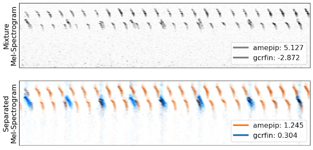
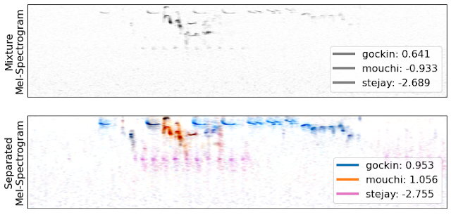
In previous competitions, we used metrics like the F1 score, which requires choosing specific detection thresholds for the models. This requires significant effort, and makes it difficult to assess the underlying model quality: A bad thresholding strategy on a good model may underperform. This year we are using a threshold-free model quality metric: class mean average precision. This metric treats each bird species output as a separate binary classifier to compute an average AUC score for each, and then averages these scores. Switching to an uncalibrated metric should increase the focus on core model quality by removing the need to choose a specific detection threshold.


How to get started

This will be the first Kaggle competition where participants can use the recently launched Kaggle Models platform that provides access to over 2,300 public, pre-trained models, including most of the TensorFlow Hub models. This new resource will have deep integrations with the rest of Kaggle, including Kaggle notebook, datasets, and competitions.

If you are interested in participating in this competition, a great place to get started quickly is to use our recently open-sourced Bird Vocalization Classifier model that is available on Kaggle Models. This global bird embedding and classification model provides output logits for more than 10k bird species and also creates embedding vectors that can be used for other tasks. Follow the steps shown in the figure below to use the Bird Vocalization Classifier model on Kaggle.

To try the model on Kaggle, navigate to the model here. 1) Click “New Notebook”; 2) click on the "Copy Code" button to copy the example lines of code needed to load the model; 3) click on the "Add Model" button to add this model as a data source to your notebook; and 4) paste the example code in the editor to load the model.

Alternatively, the competition starter notebook includes the model and extra code to more easily generate a competition submission.

We invite the research community to consider participating in the BirdCLEF competition. As a result of this effort, we hope that it will be easier for researchers and conservation practitioners to survey bird population trends and build effective conservation strategies.


Acknowledgements

Compiling these extensive datasets was a major undertaking, and we are very thankful to the many domain experts who helped to collect and manually annotate the data for this competition. Specifically, we would like to thank (institutions and individual contributors in alphabetic order): Julie Cattiau and Tom Denton on the Brain team, Maximilian Eibl and Stefan Kahl at Chemnitz University of Technology, Stefan Kahl and Holger Klinck from the K. Lisa Yang Center for Conservation Bioacoustics at the Cornell Lab of Ornithology, Alexis Joly and Henning Müller at LifeCLEF, Jonathan Baillie from NATURAL STATE, Hendrik Reers, Alain Jacot and Francis Cherutich from OekoFor GbR, and Willem-Pier Vellinga from xeno-canto. We would also like to thank Ian Davies from the Cornell Lab of Ornithology for allowing us to use the hero image in this post.

Source: Google AI Blog


TRILLsson: Small, Universal Speech Representations for Paralinguistic Tasks

In recent years, we have seen dramatic improvements on lexical tasks such as automatic speech recognition (ASR). However, machine systems still struggle to understand paralinguistic aspects — such as tone, emotion, whether a speaker is wearing a mask, etc. Understanding these aspects represents one of the remaining difficult problems in machine hearing. In addition, state-of-the-art results often come from ultra-large models trained on private data, making them impractical to run on mobile devices or to release publicly.

In “Universal Paralinguistic Speech Representations Using Self-Supervised Conformers”, to appear in ICASSP 2022, we introduce CAP12— the 12th layer of a 600M parameter model trained on the YT-U training dataset using self-supervision. We demonstrate that the CAP12 model outperforms nearly all previous results in our paralinguistic benchmark, sometimes by large margins, even though previous results are often task-specific. In “TRILLsson: Distilled Universal Paralinguistic Speech Representations'', we introduce the small, performant, publicly-available TRILLsson models and demonstrate how we reduced the size of the high-performing CAP12 model by 6x-100x while maintaining 90-96% of the performance. To create TRILLsson, we apply knowledge distillation on appropriately-sized audio chunks and use different architecture types to train smaller, faster networks that are small enough to run on mobile devices.

1M-Hour Dataset to Train Ultra-Large Self-Supervised Models
We leverage the YT-U training dataset to train the ultra-large, self-supervised CAP12 model. The YT-U dataset is a highly varied, 900M+ hour dataset that contains audio of various topics, background conditions, and speaker acoustic properties.

Video categories by length (outer) and number (inner), demonstrating the variety in the YT-U dataset (figure from BigSSL)

We then modify a Wav2Vec 2.0 self-supervised training paradigm, which can solve tasks using raw data without labels, and combine it with ultra-large Conformer models. Because self-training doesn't require labels, we can take full advantage of YT-U by scaling up our models to some of the largest model sizes ever trained, including 600M, 1B, and 8B parameters.

NOSS: A Benchmark for Paralinguistic Tasks
We demonstrate that an intermediate representation of one of the previous models contains a state-of-the-art representation for paralinguistic speech. We call the 600M parameter Conformer model without relative attention Conformer Applied to Paralinguistics (CAP). We exhaustively search through all intermediate representations of six ultra-large models and find that layer 12 (CAP12) outperforms previous representations by significant margins.

To measure the quality of the roughly 300 candidate paralinguistic speech representations, we evaluate on an expanded version of the NOn-Semantic Speech (NOSS) benchmark, which is a collection of well-studied paralinguistic speech tasks, such as speech emotion recognition, language identification, and speaker identification. These tasks focus on paralinguistics aspects of speech, which require evaluating speech features on the order of 1 second or longer, rather than lexical features, which require 100ms or shorter. We then add to the benchmark a mask-wearing task introduced at Interspeech 2020, a fake speech detection task (ASVSpoof 2019), a task to detect the level of dysarthria from project Euphonia, and an additional speech emotion recognition task (IEMOCAP). By expanding the benchmark and increasing the diversity of the tasks, we empirically demonstrate that CAP12 is even more generally useful than previous representations.

Simple linear models on time-averaged CAP12 representations even outperform complex, task-specific models on five out of eight paralinguistic tasks. This is surprising because comparable models sometimes use additional modalities (e.g., vision and speech, or text and speech) as well. Furthermore, CAP12 is exceptionally good at emotion recognition tasks. CAP12 embeddings also outperform all other embeddings on all other tasks with only a single exception: for one embedding from a supervised network on the dysarthria detection task.

Model Voxceleb   Voxforge   Speech Commands   ASVSpoof2019∗∗   Euphonia#   CREMA-D   IEMOCAP
Prev SoTA - 95.4 97.9 5.11 45.9 74.0 67.6+
TRILL 12.6 84.5 77.6 74.6 48.1 65.7 54.3
ASR Embedding 5.2 98.9 96.1 11.2 54.5 71.8 65.4
Wav2Vec2 layer 6†† 17.9 98.5 95.0 6.7 48.2 77.4 65.8
CAP12 51.0 99.7 97.0 2.5 51.5 88.2 75.0
Test performance on the NOSS Benchmark and extended tasks. “Prev SoTA” indicates the previous best performing state-of-the-art model, which has arbitrary complexity, but all other rows are linear models on time-averaged input. Filtered according to YouTube’s privacy guidelines. ∗∗ Uses equal error rate [20]. # The only non-public dataset. We exclude it from aggregate scores. Audio and visual features used in previous state-of-the-art models. + The previous state-of-the-art model performed cross-validation. For our evaluation, we hold out two specific speakers as a test. †† Wav2Vec 2.0 model from HuggingFace. Best overall layer was layer 6.

TRILLsson: Small, High Quality, Publicly Available Models
Similar to FRILL, our next step was to make an on-device, publicly available version of CAP12. This involved using knowledge distillation to train smaller, faster, mobile-friendly architectures. We experimented with EfficientNet, Audio Spectrogram Transformer (AST), and ResNet. These model types are very different, and cover both fixed-length and arbitrary-length inputs. EfficientNet comes from a neural architecture search over vision models to find simultaneously performant and efficient model structures. AST models are transformers adapted to audio inputs. ResNet is a standard architecture that has shown good performance across many different models.

We trained models that performed on average 90-96% as well as CAP12, despite being 1%-15% the size and trained using only 6% the data. Interestingly, we found that different architecture types performed better at different sizes. ResNet models performed best at the low end, EfficientNet in the middle, and AST models at the larger end.

Aggregate embedding performance vs. model size for various student model architectures and sizes. We demonstrate that ResNet architectures perform best for small sizes, EfficientNetV2 performs best in the midsize model range, up to the largest model size tested, after which the larger AST models are best.

We perform knowledge distillation with the goal of matching a student, with a fixed-size input, to the output of a teacher, with a variable-size input, for which there are two methods of generating student targets: global matching and local matching. Global matching produces distillation targets by generating CAP12 embeddings for an entire audio clip, and then requires that a student match the target from just a small segment of audio (e.g., 2 seconds). Local matching requires that the student network match the average CAP12 embedding just over the smaller portion of the audio that the student sees. In our work, we focused on local matching.

Two types of generating distillation targets for sequences. Left: Global matching uses the average CAP12 embedding over the whole clip for the target for each local chunk. Right: Local matching uses CAP12 embeddings averaged just over local clips as the distillation target.

Observation of Bimodality and Future Directions
Paralinguistic information shows an unexpected bimodal distribution. For the CAP model that operates on 500 ms input segments, and two of the full-input Conformer models, intermediate representations gradually increase in paralinguistic information, then decrease, then increase again, and finally lose this information towards the output layer. Surprisingly, this pattern is also seen when exploring the intermediate representations of networks trained on retinal images.

500 ms inputs to CAP show a relatively pronounced bimodal distribution of paralinguistic information across layers.
Two of the conformer models with full inputs show a bimodal distribution of paralinguistic information across layers.

We hope that smaller, faster models for paralinguistic speech unlock new applications in speech recognition, text-to-speech generation, and understanding user intent. We also expect that smaller models will be more easily interpretable, which will allow researchers to understand what aspects of speech are important for paralinguistics. Finally, we hope that our open-sourced speech representations are used by the community to improve paralinguistic speech tasks and user understanding in private or small datasets.

Acknowledgements
I'd like to thank my co-authors Aren Jansen, Wei Han, Daniel Park, Yu Zhang, and Subhashini Venugopalan for their hard work and creativity on this project. I'd also like to thank the members of the large collaboration for the BigSSL work, without which these projects would not be possible. The team includes James Qin, Anmol Gulati, Yuanzhong Xu, Yanping Huang, Shibo Wang, Zongwei Zhou, Bo Li, Min Ma, William Chan, Jiahui Yu, Yongqiang Wang, Liangliang Cao, Khe Chai Sim, Bhuvana Ramabhadran, Tara N. Sainath, Françoise Beaufays, Zhifeng Chen, Quoc V. Le, Chung-Cheng Chiu, Ruoming Pang, and Yonghui Wu.

Source: Google AI Blog


Separating Birdsong in the Wild for Classification

Birds are all around us, and just by listening, we can learn many things about our environment. Ecologists use birds to understand food systems and forest health — for example, if there are more woodpeckers in a forest, that means there’s a lot of dead wood. Because birds communicate and mark territory with songs and calls, it’s most efficient to identify them by ear. In fact, experts may identify up to 10x as many birds by ear as by sight.

In recent years, autonomous recording units (ARUs) have made it easy to capture thousands of hours of audio in forests that could be used to better understand ecosystems and identify critical habitat. However, manually reviewing the audio data is very time consuming, and experts in birdsong are rare. But an approach based on machine learning (ML) has the potential to greatly reduce the amount of expert review needed for understanding a habitat.

However, ML-based audio classification of bird species can be challenging for several reasons. For one, birds often sing over one another, especially during the “dawn chorus” when many birds are most active. Also, there aren’t clear recordings of individual birds to learn from — almost all of the available training data is recorded in noisy outdoor conditions, where other sounds from the wind, insects, and other environmental sources are often present. As a result, existing birdsong classification models struggle to identify quiet, distant and overlapping vocalizations. Additionally, some of the most common species often appear unlabeled in the background of training recordings for less common species, leading models to discount the common species. These difficult cases are very important for ecologists who want to identify endangered or invasive species using automated systems.

To address the general challenge of training ML models to automatically separate audio recordings without access to examples of isolated sounds, we recently proposed a new unsupervised method called mixture invariant training (MixIT) in our paper, “Unsupervised Sound Separation Using Mixture Invariant Training”. Moreover, in our new paper, “Improving Bird Classification with Unsupervised Sound Separation,” we use MixIT training to separate birdsong and improve species classification. We found that including the separated audio in the classification improves precision and classification quality on three independent soundscape datasets. We are also happy to announce the open-source release of the birdsong separation models on GitHub.

Bird Song Audio Separation
MixIT learns to separate single-channel recordings into multiple individual tracks, and can be trained entirely with noisy, real-world recordings. To train the separation model, we create a “mixture of mixtures” (MoM) by mixing together two real-world recordings. The separation model then learns to take the MoM apart into many channels to minimize a loss function that uses the two original real-world recordings as ground-truth references. The loss function uses these references to group the separated channels such that they can be mixed back together to recreate the two original real-world recordings. Since there’s no way to know how the different sounds in the MoM were grouped together in the original recordings, the separation model has no choice but to separate the individual sounds themselves, and thus learns to place each singing bird in a different output audio channel, also separate from wind and other background noise.

We trained a new MixIT separation model using birdsong recordings from Xeno-Canto and the Macaulay Library. We found that for separating birdsong, this new model outperformed a MixIT separation model trained on a large amount of general audio from the AudioSet dataset. We measure the quality of the separation by mixing two recordings together, applying separation, and then remixing the separated audio channels such that they reconstruct the original two recordings. We measure the signal-to-noise ratio (SNR) of the remixed audio relative to the original recordings. We found that the model trained specifically for birds achieved 6.1 decibels (dB) better SNR than the model trained on AudioSet (10.5 dB vs 4.4 dB). Subjectively, we also found many examples where the system worked incredibly well, separating very difficult to distinguish calls in real-world data.

The following videos demonstrate separation of birdsong from two different regions (Caples and the High Sierras). The videos show the mel-spectrogram of the mixed audio (a 2D image that shows the frequency content of the audio over time) and highlight the audio separated into different tracks.

High Sierras
  
Caples

Classifying Bird Species
To classify birds in real-world audio captured with ARUs, we first split the audio into five-second segments and then create a mel-spectrogram of each segment. We then train an EfficientNet classifier to identify bird species from the mel-spectrogram images, training on audio from Xeno-Canto and the Macaulay Library. We trained two separate classifiers, one for species in the Sierra Nevada mountains and one for upstate New York. Note that these classifiers are not trained on separated audio; that’s an area for future improvement.

We also introduced some new techniques to improve classifier training. Taxonomic training asks the classifier to provide labels for each level of the species taxonomy (genus, family, and order), which allows the model to learn groupings of species before learning the sometimes-subtle differences between similar species. Taxonomic training also allows the model to benefit from expert information about the taxonomic relationships between different species. We also found that random low-pass filtering was helpful for simulating distant sounds during training: As an audio source gets further away, the high-frequency parts fade away before the low-frequency parts. This was particularly effective for identifying species from the High Sierras region, where bird songs cover very long distances, unimpeded by trees.

Classifying Separated Audio
We found that separating audio with the new MixIT model before classification improved the classifier performance on three independent real-world datasets. The separation was particularly successful for identification of quiet and background birds, and in many cases helped with overlapping vocalizations as well.

Top: A mel-spectrogram of two birds, an American pipit (amepip) and gray-crowned rosy finch (gcrfin), from the Sierra Nevadas. The legend shows the log-probabilities for the two species given by the pre-trained classifiers. Higher values indicate more confidence, and values greater than -1.0 are usually correct classifications. Bottom: A mel-spectrogram for the automatically separated audio, with the classifier log probabilities from the separated channels. Note that the classifier only identifies the gcrfin once the audio is separated.
Top: A complex mixture with three vocalizations: A golden-crowned kinglet (gockin), mountain chickadee (mouchi), and Steller’s jay (stejay). Bottom: Separation into three channels, with classifier log probabilities for the three species. We see good visual separation of the Steller’s jay (shown by the distinct pink marks), even though the classifier isn’t sure what it is.

The separation model does have some potential limitations. Occasionally we observe over-separation, where a single song is broken into multiple channels, which can cause misclassifications. We also notice that when multiple birds are vocalizing, the most prominent song often gets a lower score after separation. This may be due to loss of environmental context or other artifacts introduced by separation that do not appear during classifier training. For now, we get the best results by running the classifier on the separated channels and the original audio, and taking the maximum score for each species. We expect that further work will allow us to reduce over-separation and find better ways to combine separation and classification. You can see and hear more examples of the full system at our GitHub repo.

Future Directions
We are currently working with partners at the California Academy of Sciences to understand how habitat and species mix changes after prescribed fires and wildfires, applying these models to ARU audio collected over many years.

We also foresee many potential applications for the unsupervised separation models in ecology, beyond just birds. For example, the separated audio can be used to create better acoustic indices, which could measure ecosystem health by tracking the total activity of birds, insects, and amphibians without identifying particular species. Similar methods could also be adapted for use underwater to track coral reef health.

Acknowledgements
We would like to thank Mary Clapp, Jack Dumbacher, and Durrell Kapan from the California Academy of Sciences for providing extensive annotated soundscapes from the Sierra Nevadas. Stefan Kahl and Holger Klinck from the Cornell Lab of Ornithology provided soundscapes from Sapsucker Woods. Training data for both the separation and classification models came from Xeno-Canto and the Macaulay Library. Finally, we would like to thank Julie Cattiau, Lauren Harrell, Matt Harvey, and our co-author, John Hershey, from the Google Bioacoustics and Sound Separation teams.

Source: Google AI Blog


Acoustic Detection of Humpback Whales Using a Convolutional Neural Network


Over the last several years, Google AI Perception teams have developed techniques for audio event analysis that have been applied on YouTube for non-speech captions, video categorizations, and indexing. Furthermore, we have published the AudioSet evaluation set and open-sourced some model code in order to further spur research in the community. Recently, we’ve become increasingly aware that many conservation organizations were collecting large quantities of acoustic data, and wondered whether it might be possible to apply these same technologies to that data in order to assist wildlife monitoring and conservation.

As part of our AI for Social Good program, and in partnership with the Pacific Islands Fisheries Science Center of the U.S. National Oceanic and Atmospheric Administration (NOAA), we developed algorithms to identify humpback whale calls in 15 years of underwater recordings from a number of locations in the Pacific. The results of this research provide new and important information about humpback whale presence, seasonality, daily calling behavior, and population structure. This is especially important in remote, uninhabited islands, about which scientists have had no information until now. Additionally, because the dataset spans a large period of time, knowing when and where humpback whales are calling will provide information on whether or not the animals have changed their distribution over the years, especially in relation to increasing human ocean activity. That information will be a key ingredient for effective mitigation of anthropogenic impacts on humpback whales.
HARP deployment locations. Green: sites with currently active recorders. Red: previous recording sites.
Passive Acoustic Monitoring and the NOAA HARP Dataset
Passive acoustic monitoring is the process of listening to marine mammals with underwater microphones called hydrophones, which can be used to record signals so that detection, classification, and localization tasks can be done offline. This has some advantages over ship-based visual surveys, including the ability to detect submerged animals, longer detection ranges and longer monitoring periods. Since 2005, NOAA has collected recordings from ocean-bottom hydrophones at 12 sites in the Pacific Island region, a winter breeding and calving destination for certain populations of humpback whales.

The data was recorded on devices called high-frequency acoustic recording packages, or HARPs (Wiggins and Hildebrand, 2007; full text PDF). In total, NOAA provided about 15 years of audio, or 9.2 terabytes after decimation from 200 kHz to 10kHz. (Since most of the sound energy in humpback vocalizations is in the 100Hz-2000Hz range, little is lost in using the lower sample rate.)

From a research perspective, identifying species of interest in such large volumes of data is an important first stage that provides input for higher-level population abundance, behavioral or oceanographic analyses. However, manually marking humpback whale calls, even with the aid of currently available computer-assisted methods, is extremely time-consuming.

Supervised Learning: Optimizing an Image Model for Humpback Detection
We made the common choice of treating audio event detection as an image classification problem, where the image is a spectrogram — a histogram of sound power plotted on time-frequency axes.
Example spectrograms of audio events found in the dataset, with time on the x-axis and frequency on the y-axis. Left: a humpback whale call (in particular, a tonal unit), Center: narrow-band noise from an unknown source, Right: hard disk noise from the HARP
This is a good representation for an image classifier, whose goal is to discriminate, because the different spectra (frequency decompositions) and time variations thereof (which are characteristic of distinct sound types) are represented in the spectrogram as visually dissimilar patterns. For the image model itself, we used ResNet-50, a convolutional neural network architecture typically used for image classification that has shown success at classifying non-speech audio. This is a supervised learning setup, where only manually labeled data could be used for training (0.2% of the entire dataset — in the next section, we describe an approach that makes use of the unlabeled data.)

The process of going from waveform to spectrogram involves choices of parameters and gain-scaling functions. Common default choices (one of which was logarithmic compression) were a good starting point, but some domain-specific tuning was needed to optimize the detection of whale calls. Humpback vocalizations are varied, but sustained, frequency-modulated, tonal units occur frequently in time. You can listen to an example below:


If the frequency didn't vary at all, a tonal unit would appear in the spectrogram as a horizontal bar. Since the calls are frequency-modulated, we actually see arcs instead of bars, but parts of the arcs are close to horizontal.

A challenge particular to this dataset was narrow-band noise, most often caused by nearby boats and the equipment itself. In a spectrogram it appears as horizontal lines, and early versions of the model would confuse it with humpback calls. This motivated us to try per-channel energy normalization (PCEN), which allows the suppression of stationary, narrow-band noise. This proved to be critical, providing a 24% reduction in error rate of whale call detection.
Spectrograms of the same 5-unit excerpt from humpback whale song beginning at 0:06 in the above recording. Top: PCEN. Bottom: log of squared magnitude. The dark blue horizontal bar along the bottom under log compression has become much lighter relative to the whale call when using PCEN
Aside from PCEN, averaging predictions over a longer period of time led to much better precision. This same effect happens for general audio event detection, but for humpback calls the increase in precision was surprisingly large. A likely explanation is that the vocalizations in our dataset are mainly in the context of whale song, a structured sequence of units than can last over 20 minutes. At the end of one unit in a song, there is a good chance another unit begins within two seconds. The input to the image model covers a short time window, but because the song is so long, model outputs from more distant time windows give extra information useful for making the correct prediction for the current time window.

Overall, evaluating on our test set of 75-second audio clips, the model identifies whether a clip contains humpback calls at over 90% precision and 90% recall. However, one should interpret these results with care; training and test data come from similar equipment and environmental conditions. That said, preliminary checks against some non-NOAA sources look promising.

Unsupervised Learning: Representation for Finding Similar Song Units
A different way to approach the question, "Where are all the humpback sounds in this data?", is to start with several examples of humpback sound and, for each of these, find more in the dataset that are similar to that example. The definition of similar here can be learned by the same ResNet we used when this was framed as a supervised problem. There, we used the labels to learn a classifier on top of the ResNet output. Here, we encourage a pair of ResNet output vectors to be close in Euclidean distance when the corresponding audio examples are close in time. With that distance function, we can retrieve many more examples of audio similar to a given one. In the future, this may be useful input for a classifier that distinguishes different humpback unit types from each other.

To learn the distance function, we used a method described in "Unsupervised Learning of Semantic Audio Representations", based on the idea that closeness in time is related to closeness in meaning. It randomly samples triplets, where each triplet is defined to consist of an anchor, a positive, and a negative. The positive and the anchor are sampled so that they start around the same time. An example of a triplet in our application would be a humpback unit (anchor), a probable repeat of the same unit by the same whale (positive) and background noise from some other month (negative). Passing the 3 samples through the ResNet (with tied weights) represents them as 3 vectors. Minimizing a loss that forces the anchor-negative distance to exceed the anchor-positive distance by a margin learns a distance function faithful to semantic similarity.

Principal component analysis (PCA) on a sample of labeled points lets us visualize the results. Separation between humpback and non-humpback is apparent. Explore for yourself using the TensorFlow Embedding Projector. Try changing Color by to each of class_label and site. Also, try changing PCA to t-SNE in the projector for a visualization that prioritizes preserving relative distances rather than sample variance.
A sample of 5000 data points in the unsupervised representation. (Orange: humpback. Blue: not humpback.)
Given individual "query" units, we retrieved the nearest neighbors in the entire corpus using Euclidean distance between embedding vectors. In some cases we found hundreds more instances of the same unit with good precision.
Manually chosen query units (boxed) and nearest neighbors using the unsupervised representation.
We intend to use these in the future to build a training set for a classifier that discriminates between song units. We could also use them to expand the training set used for learning a humpback detector.

Predictions from the Supervised Classifier on the Entire Dataset
We plotted summaries of the model output grouped by time and location. Not all sites had deployments in all years. Duty cycling (example: 5 minutes on, 15 minutes off) allows longer deployments on limited battery power, but the schedule can vary. To deal with these sources of variability, we consider the proportion of sampled time in which humpback calling was detected to the total time recorded in a month:
Time density of presence on year / month axes for the Kona and Saipan sites.
The apparent seasonal variation is consistent with a known pattern in which humpback populations spend summers feeding near Alaska and then migrate to the vicinity of the Hawaiian Islands to breed and give birth. This is a nice sanity check for the model.

We hope the predictions for the full dataset will equip experts at NOAA to reach deeper insights into the status of these populations and into the degree of any anthropogenic impacts on them. We also hope this is just one of the first few in a series of successes as Google works to accelerate the application of machine learning to the world's biggest humanitarian and environmental challenges.

Acknowledgements
We would like to thank Ann Allen (NOAA Fisheries) for providing the bulk of the ground truth data, for many useful rounds of feedback, and for some of the words in this post. Karlina Merkens (NOAA affiliate) provided further useful guidance. We also thank the NOAA Pacific Islands Fisheries Science Center as a whole for collecting and sharing the acoustic data.

Within Google, Jiayang Liu, Julie Cattiau, Aren Jansen, Rif A. Saurous, and Lauren Harrell contributed to this work. Special thanks go to Lauren, who designed the plots in the analysis section and implemented them using ggplot.

Source: Google AI Blog


Adding Sound Effect Information to YouTube Captions


The effect of audio on our perception of the world can hardly be overstated. Its importance as a communication medium via speech is obviously the most familiar, but there is also significant information conveyed by ambient sounds. These ambient sounds create context that we instinctively respond to, like getting startled by sudden commotion, the use of music as a narrative element, or how laughter is used as an audience cue in sitcoms.

Since 2009, YouTube has provided automatic caption tracks for videos, focusing heavily on speech transcription in order to make the content hosted more accessible. However, without similar descriptions of the ambient sounds in videos, much of the information and impact of a video is not captured by speech transcription alone. To address this, we announced the addition of sound effect information to the automatic caption track in YouTube videos, enabling greater access to the richness of all the audio content.

In this post, we discuss the backend system developed for this effort, a collaboration among the Accessibility, Sound Understanding and YouTube teams that used machine learning (ML) to enable the first ever automatic sound effect captioning system for YouTube.
Click the CC button to see the sound effect captioning system in action.
The application of ML – in this case, a Deep Neural Network (DNN) model – to the captioning task presented unique challenges. While the process of analyzing the time-domain audio signal of a video to detect various ambient sounds is similar to other well known classification problems (such as object detection in images), in a product setting the solution faces additional difficulties. In particular, given an arbitrary segment of audio, we need our models to be able to 1) detect the desired sounds, 2) temporally localize the sound in the segment and 3) effectively integrate it in the caption track, which may have parallel and independent speech recognition results.

A DNN Model for Ambient Sound
The first challenge we faced in developing the model was the task of obtaining enough labeled data suitable for training our neural network. While labeled ambient sound information is difficult to come by, we were able to generate a large enough dataset for training using weakly labeled data. But of all the ambient sounds in a given video, which ones should we train our DNN to detect?

For the initial launch of this feature, we chose [APPLAUSE], [MUSIC] and [LAUGHTER], prioritized based upon our analysis of human-created caption tracks that indicates that they are among the most frequent sounds that are manually captioned. While the sound space is obviously far richer and provides even more contextually relevant information than these three classes, the semantic information conveyed by these sound effects in the caption track is relatively unambiguous, as opposed to sounds like [RING] which raises the question of “what was it that rang – a bell, an alarm, a phone?”

Much of our initial work on detecting these ambient sounds also included developing the infrastructure and analysis frameworks to enable scaling for future work, including both the detection of sound events and their integration into the automatic caption track. Investing in the development of this infrastructure has the added benefit of allowing us to easily incorporate more sound types in the future, as we expand our algorithms to understand a wider vocabulary of sounds (e.g. [RING], [KNOCK], [BARK]). In doing so, we will be able to incorporate the detected sounds into the narrative to provide more relevant information (e.g. [PIANO MUSIC], [RAUCOUS APPLAUSE]) to viewers.

Dense Detections to Captions
When a video is uploaded to YouTube, the sound effect recognition pipeline runs on the audio stream in the video. The DNN looks at short segments of audio and predicts whether that segment contains any one of the sound events of interest – since multiple sound effects can co-occur, our model makes a prediction at each time step for each of the sound effects. The segment window is then slid to the right (i.e. a slightly later point in time) and the model is used to make a prediction again, and so on till it reaches the end. This results in a dense stream the (likelihood of) presence of each of the sound events in our vocabulary at 100 frames per second.

The dense prediction stream is not directly exposed to the user, of course, since that would result in captions flickering on and off, and because we know that a number of sound effects have some degree of temporal continuity when they occur; e.g. “music” and “applause” will usually be present for a few seconds at least. To incorporate this intuition, we smooth over the dense prediction stream using a modified Viterbi algorithm containing two states: ON and OFF, with the predicted segments for each sound effect corresponding to the ON state. The figure below provides an illustration of the process in going from the dense detections to the final segments determined to contain sound effects of interest.
(Left) The dense sequence of probabilities from our DNN for the occurrence over time of single sound category in a video. (Center) Binarized segments based on the modified Viterbi algorithm. (Right) The duration-based filter removes segments that are shorter in duration than desired for the class.
A classification-based system such as this one will certainly have some errors, and needs to be able to trade off false positives against missed detections as per the product goals. For example, due to the weak labels in the training dataset, the model was often confused between events that tended to co-occur. For example, a segment labeled “laugh” would usually contain both speech and laughter and the model for “laugh” would have a hard time distinguishing them in test data. In our system, we allow further restrictions based on time spent in the ON state (i.e. do not determine sound X to be detected unless it was determined to be present for at least Y seconds) to push performance toward a desired point in the precision-recall curve.

Once we were satisfied with the performance of our system in temporally localizing sound effect captions based on our offline evaluation metrics, we were faced with the following: how do we combine the sound effect and speech captions to create a single automatic caption track, and how (or when) do we present sound effect information to the user to make it most useful to them?

Adding Sound Effect Information into the Automatic Captions Track
Once we had a system capable of accurately detecting and classifying the ambient sounds in video, we investigated how to convey that information to the viewer in an effective way. In collaboration with our User Experience (UX) research teams, we explored various design options and tested them in a qualitative pilot usability study. The participants of the study had different hearing levels and varying needs for captions. We asked participants a number of questions including whether it improved their overall experience, their ability to follow events in the video and extract relevant information from the caption track, to understand the effect of variables such as:
  • Using separate parts of the screen for speech and sound effect captions.
  • Interleaving the speech and sound effect captions as they occur.
  • Only showing sound effect captions at the end of sentences or when there is a pause in speech (even if they occurred in the middle of speech).
  • How hearing users perceive captions when watching with the sound off.
While it wasn’t surprising that almost all users appreciated the added sound effect information when it was accurate, we also paid specific attention to the feedback when the sound detection system made an error (a false positive when determining presence of a sound, or failing to detect an occurrence). This presented a surprising result: when sound effect information was incorrect, it did not detract from the participant’s experience in roughly 50% of the cases. Based upon participant feedback, the reasons for this appear to be:
  • Participants who could hear the audio were able to ignore the inaccuracies.
  • Participants who could not hear the audio interpreted the error as the presence of a sound event, and that they had not missed out on critical speech information.
Overall, users reported that they would be fine with the system making the occasional mistake as long as it was able to provide good information far more often than not.

Looking Forward
Our work toward enabling automatic sound effect captions for YouTube videos and the initial rollout is a step toward making the richness of content in videos more accessible to our users who experience videos in different ways and in different environments that require captions. We’ve developed a framework to enrich the automatic caption track with sound effects, but there is still much to be done here. We hope that this will spur further work and discussion in the community around improving captions using not only automatic techniques, but also around ways to make creator-generated and community-contributed caption tracks richer (including perhaps, starting with the auto-captions) and better to further improve the viewing experience for our users.