 Here are Google’s latest AI updates from May 2026
The latest AI news we announced in May 2026
Here are Google’s latest AI updates from May 2026
Here are Google’s latest AI updates from May 2026
 Google and the Utah State Board of Education partner to bring Gemini for Education to educators and students statewide.

The Dev channel has been updated to 151.0.7872.0 for Windows, Mac and Linux.
A partial list of changes is available in the Git log. Interested in switching release channels? Find out how. If you find a new issue, please let us know by filing a bug. The community help forum is also a great place to reach out for help or learn about common issues.
Chrome Release Team
Google Chrome
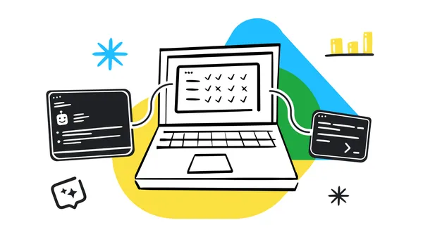 Today, we’re launching local development for Kaggle Benchmarks.
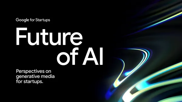 We’re sharing our findings in Google for Startups’ latest report, the Future of AI: Perspectives on generative media for startups.
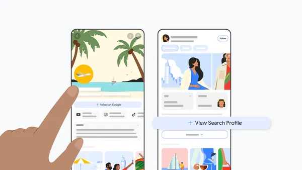 We’re introducing a new, dedicated space for creators, publishers and brands.
Hi everyone! We've just released Chrome Dev 151 (151.0.7872.3) for Android. It's now available on Google Play.
You can see a partial list of the changes in the Git log. For details on new features, check out the Chromium blog, and for details on web platform updates, check here.
If you find a new issue, please let us know by filing a bug.
Chrome Release Team
Google Chrome
 Kameirah, a high school senior from Washington, shares more about the inspiration behind her winning Doodle.
 Google and Intersect are announcing construction of the Meitner Energy Center, a new data center and new energy generation in Texas.