Tag Archives: Unsupervised Learning

Differentially private clustering for large-scale datasets

Clustering is a central problem in unsupervised machine learning (ML) with many applications across domains in both industry and academic research more broadly. At its core, clustering consists of the following problem: given a set of data elements, the goal is to partition the data elements into groups such that similar objects are in the same group, while dissimilar objects are in different groups. This problem has been studied in math, computer science, operations research and statistics for more than 60 years in its myriad variants. Two common forms of clustering are metric clustering, in which the elements are points in a metric space, like in the k-means problem, and graph clustering, where the elements are nodes of a graph whose edges represent similarity among them.

In the k-means clustering problem, we are given a set of points in a metric space with the objective to identify k representative points, called centers (here depicted as triangles), so as to minimize the sum of the squared distances from each point to its closest center. Source, rights: CC-BY-SA-4.0

Despite the extensive literature on algorithm design for clustering, few practical works have focused on rigorously protecting the user's privacy during clustering. When clustering is applied to personal data (e.g., the queries a user has made), it is necessary to consider the privacy implications of using a clustering solution in a real system and how much information the output solution reveals about the input data.

To ensure privacy in a rigorous sense, one solution is to develop differentially private (DP) clustering algorithms. These algorithms ensure that the output of the clustering does not reveal private information about a specific data element (e.g., whether a user has made a given query) or sensitive data about the input graph (e.g., a relationship in a social network). Given the importance of privacy protections in unsupervised machine learning, in recent years Google has invested in research on theory and practice of differentially private metric or graph clustering, and differential privacy in a variety of contexts, e.g., heatmaps or tools to design DP algorithms.

Today we are excited to announce two important updates: 1) a new differentially-private algorithm for hierarchical graph clustering, which we’ll be presenting at ICML 2023, and 2) the open-source release of the code of a scalable differentially-private k-means algorithm. This code brings differentially private k-means clustering to large scale datasets using distributed computing. Here, we will also discuss our work on clustering technology for a recent launch in the health domain for informing public health authorities.


Differentially private hierarchical clustering

Hierarchical clustering is a popular clustering approach that consists of recursively partitioning a dataset into clusters at an increasingly finer granularity. A well known example of hierarchical clustering is the phylogenetic tree in biology in which all life on Earth is partitioned into finer and finer groups (e.g., kingdom, phylum, class, order, etc.). A hierarchical clustering algorithm receives as input a graph representing the similarity of entities and learns such recursive partitions in an unsupervised way. Yet at the time of our research no algorithm was known to compute hierarchical clustering of a graph with edge privacy, i.e., preserving the privacy of the vertex interactions.

In “Differentially-Private Hierarchical Clustering with Provable Approximation Guarantees”, we consider how well the problem can be approximated in a DP context and establish firm upper and lower bounds on the privacy guarantee. We design an approximation algorithm (the first of its kind) with a polynomial running time that achieves both an additive error that scales with the number of nodes n (of order n2.5) and a multiplicative approximation of O(log½ n), with the multiplicative error identical to the non-private setting. We further provide a new lower bound on the additive error (of order n2) for any private algorithm (irrespective of its running time) and provide an exponential-time algorithm that matches this lower bound. Moreover, our paper includes a beyond-worst-case analysis focusing on the hierarchical stochastic block model, a standard random graph model that exhibits a natural hierarchical clustering structure, and introduces a private algorithm that returns a solution with an additive cost over the optimum that is negligible for larger and larger graphs, again matching the non-private state-of-the-art approaches. We believe this work expands the understanding of privacy preserving algorithms on graph data and will enable new applications in such settings.


Large-scale differentially private clustering

We now switch gears and discuss our work for metric space clustering. Most prior work in DP metric clustering has focused on improving the approximation guarantees of the algorithms on the k-means objective, leaving scalability questions out of the picture. Indeed, it is not clear how efficient non-private algorithms such as k-means++ or k-means// can be made differentially private without sacrificing drastically either on the approximation guarantees or the scalability. On the other hand, both scalability and privacy are of primary importance at Google. For this reason, we recently published multiple papers that address the problem of designing efficient differentially private algorithms for clustering that can scale to massive datasets. Our goal is, moreover, to offer scalability to large scale input datasets, even when the target number of centers, k, is large.

We work in the massively parallel computation (MPC) model, which is a computation model representative of modern distributed computation architectures. The model consists of several machines, each holding only part of the input data, that work together with the goal of solving a global problem while minimizing the amount of communication between machines. We present a differentially private constant factor approximation algorithm for k-means that only requires a constant number of rounds of synchronization. Our algorithm builds upon our previous work on the problem (with code available here), which was the first differentially-private clustering algorithm with provable approximation guarantees that can work in the MPC model.

The DP constant factor approximation algorithm drastically improves on the previous work using a two phase approach. In an initial phase it computes a crude approximation to “seed” the second phase, which consists of a more sophisticated distributed algorithm. Equipped with the first-step approximation, the second phase relies on results from the Coreset literature to subsample a relevant set of input points and find a good differentially private clustering solution for the input points. We then prove that this solution generalizes with approximately the same guarantee to the entire input.


Vaccination search insights via DP clustering

We then apply these advances in differentially private clustering to real-world applications. One example is our application of our differentially-private clustering solution for publishing COVID vaccine-related queries, while providing strong privacy protections for the users.

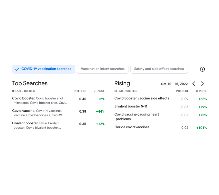
The goal of Vaccination Search Insights (VSI) is to help public health decision makers (health authorities, government agencies and nonprofits) identify and respond to communities' information needs regarding COVID vaccines. In order to achieve this, the tool allows users to explore at different geolocation granularities (zip-code, county and state level in the U.S.) the top themes searched by users regarding COVID queries. In particular, the tool visualizes statistics on trending queries rising in interest in a given locale and time.

Screenshot of the output of the tool. Displayed on the left, the top searches related to Covid vaccines during the period Oct 10-16 2022. On the right, the queries that have had rising importance during the same period and compared to the previous week.

To better help identifying the themes of the trending searches, the tool clusters the search queries based on their semantic similarity. This is done by applying a custom-designed k-means–based algorithm run over search data that has been anonymized using the DP Gaussian mechanism to add noise and remove low-count queries (thus resulting in a differentially clustering). The method ensures strong differential privacy guarantees for the protection of the user data.

This tool provided fine-grained data on COVID vaccine perception in the population at unprecedented scales of granularity, something that is especially relevant to understand the needs of the marginalized communities disproportionately affected by COVID. This project highlights the impact of our investment in research in differential privacy, and unsupervised ML methods. We are looking to other important areas where we can apply these clustering techniques to help guide decision making around global health challenges, like search queries on climate change–related challenges such as air quality or extreme heat.


Acknowledgements

We thank our co-authors Silvio Lattanzi, Vahab Mirrokni, Andres Munoz Medina, Shyam Narayanan, David Saulpic, Chris Schwiegelshohn, Sergei Vassilvitskii, Peilin Zhong and our colleagues from the Health AI team that made the VSI launch possible Shailesh Bavadekar, Adam Boulanger, Tague Griffith, Mansi Kansal, Chaitanya Kamath, Akim Kumok, Yael Mayer, Tomer Shekel, Megan Shum, Charlotte Stanton, Mimi Sun, Swapnil Vispute, and Mark Young.

For more information on the Graph Mining team (part of Algorithm and Optimization) visit our pages.

Source: Google AI Blog


Unsupervised and semi-supervised anomaly detection with data-centric ML

Anomaly detection (AD), the task of distinguishing anomalies from normal data, plays a vital role in many real-world applications, such as detecting faulty products from vision sensors in manufacturing, fraudulent behaviors in financial transactions, or network security threats. Depending on the availability of the type of data — negative (normal) vs. positive (anomalous) and the availability of their labels — the task of AD involves different challenges.

(a) Fully supervised anomaly detection, (b) normal-only anomaly detection, (c, d, e) semi-supervised anomaly detection, (f) unsupervised anomaly detection.

While most previous works were shown to be effective for cases with fully-labeled data (either (a) or (b) in the above figure), such settings are less common in practice because labels are particularly tedious to obtain. In most scenarios users have a limited labeling budget, and sometimes there aren’t even any labeled samples during training. Furthermore, even when labeled data are available, there could be biases in the way samples are labeled, causing distribution differences. Such real-world data challenges limit the achievable accuracy of prior methods in detecting anomalies.

This post covers two of our recent papers on AD, published in Transactions on Machine Learning Research (TMLR), that address the above challenges in unsupervised and semi-supervised settings. Using data-centric approaches, we show state-of-the-art results in both. In “Self-supervised, Refine, Repeat: Improving Unsupervised Anomaly Detection”, we propose a novel unsupervised AD framework that relies on the principles of self-supervised learning without labels and iterative data refinement based on the agreement of one-class classifier (OCC) outputs. In “SPADE: Semi-supervised Anomaly Detection under Distribution Mismatch”, we propose a novel semi-supervised AD framework that yields robust performance even under distribution mismatch with limited labeled samples.


Unsupervised anomaly detection with SRR: Self-supervised, Refine, Repeat

Discovering a decision boundary for a one-class (normal) distribution (i.e., OCC training) is challenging in fully unsupervised settings as unlabeled training data include two classes (normal and abnormal). The challenge gets further exacerbated as the anomaly ratio gets higher for unlabeled data. To construct a robust OCC with unlabeled data, excluding likely-positive (anomalous) samples from the unlabeled data, the process referred to as data refinement, is critical. The refined data, with a lower anomaly ratio, are shown to yield superior anomaly detection models.

SRR first refines data from an unlabeled dataset, then iteratively trains deep representations using refined data while improving the refinement of unlabeled data by excluding likely-positive samples. For data refinement, an ensemble of OCCs is employed, each of which is trained on a disjoint subset of unlabeled training data. If there is consensus among all the OCCs in the ensemble, the data that are predicted to be negative (normal) are included in the refined data. Finally, the refined training data are used to train the final OCC to generate the anomaly predictions.

Training SRR with a data refinement module (OCCs ensemble), representation learner, and final OCC. (Green/red dots represent normal/abnormal samples, respectively).

SRR results

We conduct extensive experiments across various datasets from different domains, including semantic AD (CIFAR-10, Dog-vs-Cat), real-world manufacturing visual AD (MVTec), and real-world tabular AD benchmarks such as detecting medical (Thyroid) or network security (KDD 1999) anomalies. We consider methods with both shallow (e.g., OC-SVM) and deep (e.g., GOAD, CutPaste) models. Since the anomaly ratio of real-world data can vary, we evaluate models at different anomaly ratios of unlabeled training data and show that SRR significantly boosts AD performance. For example, SRR improves more than 15.0 average precision (AP) with a 10% anomaly ratio compared to a state-of-the-art one-class deep model on CIFAR-10. Similarly, on MVTec, SRR retains solid performance, dropping less than 1.0 AUC with a 10% anomaly ratio, while the best existing OCC drops more than 6.0 AUC. Lastly, on Thyroid (tabular data), SRR outperforms a state-of-the-art one-class classifier by 22.9 F1 score with a 2.5% anomaly ratio.

Across various domains, SRR (blue line) significantly boosts AD performance with various anomaly ratios in fully unsupervised settings.

SPADE: Semi-supervised Pseudo-labeler Anomaly Detection with Ensembling

Most semi-supervised learning methods (e.g., FixMatch, VIME) assume that the labeled and unlabeled data come from the same distributions. However, in practice, distribution mismatch commonly occurs, with labeled and unlabeled data coming from different distributions. One such case is positive and unlabeled (PU) or negative and unlabeled (NU) settings, where the distributions between labeled (either positive or negative) and unlabeled (both positive and negative) samples are different. Another cause of distribution shift is additional unlabeled data being gathered after labeling. For example, manufacturing processes may keep evolving, causing the corresponding defects to change and the defect types at labeling to differ from the defect types in unlabeled data. In addition, for applications like financial fraud detection and anti-money laundering, new anomalies can appear after the data labeling process, as criminal behavior may adapt. Lastly, labelers are more confident on easy samples when they label them; thus, easy/difficult samples are more likely to be included in the labeled/unlabeled data. For example, with some crowd-sourcing–based labeling, only the samples with some consensus on the labels (as a measure of confidence) are included in the labeled set.

Three common real-world scenarios with distribution mismatches (blue box: normal samples, red box: known/easy anomaly samples, yellow box: new/difficult anomaly samples).

Standard semi-supervised learning methods assume that labeled and unlabeled data come from the same distribution, so are sub-optimal for semi-supervised AD under distribution mismatch. SPADE utilizes an ensemble of OCCs to estimate the pseudo-labels of the unlabeled data — it does this independent of the given positive labeled data, thus reducing the dependency on the labels. This is especially beneficial when there is a distribution mismatch. In addition, SPADE employs partial matching to automatically select the critical hyper-parameters for pseudo-labeling without relying on labeled validation data, a crucial capability given limited labeled data.

Block diagram of SPADE with zoom in the detailed block diagram of the proposed pseudo-labelers.

SPADE results

We conduct extensive experiments to showcase the benefits of SPADE in various real-world settings of semi-supervised learning with distribution mismatch. We consider multiple AD datasets for image (including MVTec) and tabular (including Covertype, Thyroid) data.

SPADE shows state-of-the-art semi-supervised anomaly detection performance across a wide range of scenarios: (i) new-types of anomalies, (ii) easy-to-label samples, and (iii) positive-unlabeled examples. As shown below, with new-types of anomalies, SPADE outperforms the state-of-the-art alternatives by 5% AUC on average.

AD performances with three different scenarios across various datasets (Covertype, MVTec, Thyroid) in terms of AUC. Some baselines are only applicable to some scenarios. More results with other baselines and datasets can be found in the paper.

We also evaluate SPADE on real-world financial fraud detection datasets: Kaggle credit card fraud and Xente fraud detection. For these, anomalies evolve (i.e., their distributions change over time) and to identify evolving anomalies, we need to keep labeling for new anomalies and retrain the AD model. However, labeling would be costly and time consuming. Even without additional labeling, SPADE can improve the AD performance using both labeled data and newly-gathered unlabeled data.

AD performances with time-varying distributions using two real-world fraud detection datasets with 10% labeling ratio. More baselines can be found in the paper.

As shown above, SPADE consistently outperforms alternatives on both datasets, taking advantage of the unlabeled data and showing robustness to evolving distributions.


Conclusions

AD has a wide range of use cases with significant importance in real-world applications, from detecting security threats in financial systems to identifying faulty behaviors of manufacturing machines.

One challenging and costly aspect of building an AD system is that anomalies are rare and not easily detectable by people. To this end, we have proposed SRR, a canonical AD framework to enable high performance AD without the need for manual labels for training. SRR can be flexibly integrated with any OCC, and applied on raw data or on trainable representations.

Semi-supervised AD is another highly-important challenge — in many scenarios, the distributions of labeled and unlabeled samples don’t match. SPADE introduces a robust pseudo-labeling mechanism using an ensemble of OCCs and a judicious way of combining supervised and self-supervised learning. In addition, SPADE introduces an efficient approach to pick critical hyperparameters without a validation set, a crucial component for data-efficient AD.

Overall, we demonstrate that SRR and SPADE consistently outperform the alternatives in various scenarios across multiple types of datasets.


Acknowledgements

We gratefully acknowledge the contributions of Kihyuk Sohn, Chun-Liang Li, Chen-Yu Lee, Kyle Ziegler, Nate Yoder, and Tomas Pfister.

Source: Google AI Blog


Unlocking Zero-Resource Machine Translation to Support New Languages in Google Translate

Machine translation (MT) technology has made significant advances in recent years, as deep learning has been integrated with natural language processing (NLP). Performance on research benchmarks like WMT have soared, and translation services have improved in quality and expanded to include new languages. Nevertheless, while existing translation services cover languages spoken by the majority of people world wide, they only include around 100 languages in total, just over 1% of those actively spoken globally. Moreover, the languages that are currently represented are overwhelmingly European, largely overlooking regions of high linguistic diversity, like Africa and the Americas.

There are two key bottlenecks towards building functioning translation models for the long tail of languages. The first arises from data scarcity; digitized data for many languages is limited and can be difficult to find on the web due to quality issues with Language Identification (LangID) models. The second challenge arises from modeling limitations. MT models usually train on large amounts of parallel (translated) text, but without such data, models must learn to translate from limited amounts of monolingual text, which is a novel area of research. Both of these challenges need to be addressed for translation models to reach sufficient quality.

In “Building Machine Translation Systems for the Next Thousand Languages”, we describe how to build high-quality monolingual datasets for over a thousand languages that do not have translation datasets available and demonstrate how one can use monolingual data alone to train MT models. As part of this effort, we are expanding Google Translate to include 24 under-resourced languages. For these languages, we created monolingual datasets by developing and using specialized neural language identification models combined with novel filtering approaches. The techniques we introduce supplement massively multilingual models with a self supervised task to enable zero-resource translation. Finally, we highlight how native speakers have helped us realize this accomplishment.

Meet the Data
Automatically gathering usable textual data for under-resourced languages is much more difficult than it may seem. Tasks like LangID, which work well for high-resource languages, are unsuccessful for under-resourced languages, and many publicly available datasets crawled from the web often contain more noise than usable data for the languages they attempt to support. In our early attempts to identify under-resourced languages on the web by training a standard Compact Language Detector v3 (CLD3) LangID model, we too found that the dataset was too noisy to be usable.

As an alternative, we trained a Transformer-based, semi-supervised LangID model on over 1000 languages. This model supplements the LangID task with the MAsked Sequence-to-Sequence (MASS) task to better generalize over noisy web data. MASS simply garbles the input by randomly removing sequences of tokens from it, and trains the model to predict these sequences. We applied the Transformer-based model to a dataset that had been filtered with a CLD3 model and trained to recognize clusters of similar languages.

We then applied the open sourced Term Frequency-Inverse Internet Frequency (TF-IIF) filtering to the resulting dataset to find and discard sentences that were actually in related high-resource languages, and developed a variety of language-specific filters to eliminate specific pathologies. The result of this effort was a dataset with monolingual text in over 1000 languages, of which 400 had over 100,000 sentences. We performed human evaluations on samples of 68 of these languages and found that the majority (>70%) reflected high-quality, in-language content.

The amount of monolingual data per language versus the amount of parallel (translated) data per language. A small number of languages have large amounts of parallel data, but there is a long tail of languages with only monolingual data.

Meet the Models
Once we had a dataset of monolingual text in over 1000 languages, we then developed a simple yet practical approach for zero-resource translation, i.e., translation for languages with no in-language parallel text and no language-specific translation examples. Rather than limiting our model to an artificial scenario with only monolingual text, we also include all available parallel text data with millions of examples for higher resource languages to enable the model to learn the translation task. Simultaneously, we train the model to learn representations of under-resourced languages directly from monolingual text using the MASS task. In order to solve this task, the model is forced to develop a sophisticated representation of the language in question, developing a complex understanding of how words relate to other words in a sentence.

Relying on the benefits of transfer learning in massively multilingual models, we train a single giant translation model on all available data for over 1000 languages. The model trains on monolingual text for all 1138 languages and on parallel text for a subset of 112 of the higher-resourced languages.

At training time, any input the model sees has a special token indicating which language the output should be in, exactly like the standard formulation for multilingual translation. Our additional innovation is to use the same special tokens for both the monolingual MASS task and the translation task. Therefore, the token translate_to_french may indicate that the source is in English and needs to be translated to French (the translation task), or it may mean that the source is in garbled French and needs to be translated to fluent French (the MASS task). By using the same tags for both tasks, a translate_to_french tag takes on the meaning, “Produce a fluent output in French that is semantically close to the input, regardless of whether the input is garbled in the same language or in another language entirely. From the model’s perspective, there is not much difference between the two.

Surprisingly, this simple procedure produces high quality zero-shot translations. The BLEU and ChrF scores for the resulting model are in the 10–40 and 20–60 ranges respectively, indicating mid- to high-quality translation. We observed meaningful translations even for highly inflected languages like Quechua and Kalaallisut, despite these languages being linguistically dissimilar to all other languages in the model. However, we only computed these metrics on the small subset of languages with human-translated evaluation sets. In order to understand the quality of translation for the remaining languages, we developed an evaluation metric based on round-trip translation, which allowed us to see that several hundred languages are reaching high translation quality.

To further improve quality, we use the model to generate large amounts of synthetic parallel data, filter the data based on round-trip translation (comparing a sentence translated into another language and back again), and continue training the model on this filtered synthetic data via back-translation and self-training. Finally, we fine-tune the model on a smaller subset of 30 languages and distill it into a model small enough to be served.

Translation accuracy scores for 638 of the languages supported in our model, using the metric we developed (RTTLangIDChrF), for both the higher-resource supervised languages and the low-resource zero-resource languages.

Contributions from Native Speakers
Regular communication with native speakers of these languages was critical for our research. We collaborated with over 100 people at Google and other institutions who spoke these languages. Some volunteers helped develop specialized filters to remove out-of-language content overlooked by automatic methods, for instance Hindi mixed with Sanskrit. Others helped with transliterating between different scripts used by the languages, for instance between Meetei Mayek and Bengali, for which sufficient tools didn’t exist; and yet others helped with a gamut of tasks related to evaluation. Native speakers were also key for advising in matters of political sensitivity, like the appropriate name for the language, and the appropriate writing system to use for it. And only native speakers could answer the ultimate question: given the current quality of translation, would it be valuable to the community for Google Translate to support this language?

Closing Notes
This advance is an exciting first step toward supporting more language technologies in under-resourced languages. Most importantly, we want to stress that the quality of translations produced by these models still lags far behind that of the higher-resource languages supported by Google Translate. These models are certainly a useful first tool for understanding content in under-resourced languages, but they will make mistakes and exhibit their own biases. As with any ML-driven tool, one should consider the output carefully.

The complete list of new languages added to Google Translate in this update:

Acknowledgements
We would like to thank Julia Kreutzer, Orhan Firat, Daan van Esch, Aditya Siddhant, Mengmeng Niu, Pallavi Baljekar, Xavier Garcia, Wolfgang Macherey, Theresa Breiner, Vera Axelrod, Jason Riesa, Yuan Cao, Mia Xu Chen, Klaus Macherey, Maxim Krikun, Pidong Wang, Alexander Gutkin, Apurva Shah, Yanping Huang, Zhifeng Chen, Yonghui Wu, and Macduff Hughes for their contributions to the research, engineering, and leadership of this project.

We would also like to extend our deepest gratitude to the following native speakers and members of affected communities, who helped us in a wide variety of ways: Yasser Salah Eddine Bouchareb (Algerian Arabic); Mfoniso Ukwak (Anaang); Bhaskar Borthakur, Kishor Barman, Rasika Saikia, Suraj Bharech (Assamese); Ruben Hilare Quispe (Aymara); Devina Suyanto (Balinese); Allahserix Auguste Tapo, Bakary Diarrassouba, Maimouna Siby (Bambara); Mohammad Jahangir (Baluchi); Subhajit Naskar (Bengali); Animesh Pathak, Ankur Bapna, Anup Mohan, Chaitanya Joshi, Chandan Dubey, Kapil Kumar, Manish Katiyar, Mayank Srivastava, Neeharika, Saumya Pathak, Tanya Sinha, Vikas Singh (Bhojpuri); Bowen Liang, Ellie Chio, Eric Dong, Frank Tang, Jeff Pitman, John Wong, Kenneth Chang, Manish Goregaokar, Mingfei Lau, Ryan Li, Yiwen Luo (Cantonese); Monang Setyawan (Caribbean Javanese); Craig Cornelius (Cherokee); Anton Prokopyev (Chuvash); Rajat Dogra, Sid Dogra (Dogri); Mohamed Kamagate (Dyula); Chris Assigbe, Dan Ameme, Emeafa Doe, Irene Nyavor, Thierry Gnanih, Yvonne Dumor (Ewe); Abdoulaye Barry, Adama Diallo, Fauzia van der Leeuw, Ibrahima Barry (Fulfulde); Isabel Papadimitriou (Greek); Alex Rudnick (Guarani); Mohammad Khdeir (Gulf Arabic); Paul Remollata (Hiligaynon); Ankur Bapna (Hindi); Mfoniso Ukwak (Ibibio); Nze Lawson (Igbo); D.J. Abuy, Miami Cabansay (Ilocano); Archana Koul, Shashwat Razdan, Sujeet Akula (Kashmiri); Jatin Kulkarni, Salil Rajadhyaksha, Sanjeet Hegde Desai, Sharayu Shenoy, Shashank Shanbhag, Shashi Shenoy (Konkani); Ryan Michael, Terrence Taylor (Krio); Bokan Jaff, Medya Ghazizadeh, Roshna Omer Abdulrahman, Saman Vaisipour, Sarchia Khursheed (Kurdish (Sorani));Suphian Tweel (Libyan Arabic); Doudou Kisabaka (Lingala); Colleen Mallahan, John Quinn (Luganda); Cynthia Mboli (Luyia); Abhishek Kumar, Neeraj Mishra, Priyaranjan Jha, Saket Kumar, Snehal Bhilare (Maithili); Lisa Wang (Mandarin Chinese); Cibu Johny (Malayalam); Viresh Ratnakar (Marathi); Abhi Sanoujam, Gautam Thockchom, Pritam Pebam, Sam Chaomai, Shangkar Mayanglambam, Thangjam Hindustani Devi (Meiteilon (Manipuri)); Hala Ajil (Mesopotamian Arabic); Hamdanil Rasyid (Minangkabau); Elizabeth John, Remi Ralte, S Lallienkawl Gangte,Vaiphei Thatsing, Vanlalzami Vanlalzami (Mizo); George Ouais (MSA); Ahmed Kachkach, Hanaa El Azizi (Morrocan Arabic); Ujjwal Rajbhandari (Newari); Ebuka Ufere, Gabriel Fynecontry, Onome Ofoman, Titi Akinsanmi (Nigerian Pidgin); Marwa Khost Jarkas (North Levantine Arabic); Abduselam Shaltu, Ace Patterson, Adel Kassem, Mo Ali, Yonas Hambissa (Oromo); Helvia Taina, Marisol Necochea (Quechua); AbdelKarim Mardini (Saidi Arabic); Ishank Saxena, Manasa Harish, Manish Godara, Mayank Agrawal, Nitin Kashyap, Ranjani Padmanabhan, Ruchi Lohani, Shilpa Jindal, Shreevatsa Rajagopalan, Vaibhav Agarwal, Vinod Krishnan (Sanskrit); Nabil Shahid (Saraiki); Ayanda Mnyakeni (Sesotho, Sepedi); Landis Baker (Seychellois Creole); Taps Matangira (Shona); Ashraf Elsharif (Sudanese Arabic); Sakhile Dlamini (Swati); Hakim Sidahmed (Tamazight); Melvin Johnson (Tamil); Sneha Kudugunta (Telugu); Alexander Tekle, Bserat Ghebremicael, Nami Russom, Naud Ghebre (Tigrinya); Abigail Annkah, Diana Akron, Maame Ofori, Monica Opoku-Geren, Seth Duodu-baah, Yvonne Dumor (Twi); Ousmane Loum (Wolof); and Daniel Virtheim (Yiddish).


Source: Google AI Blog


DADS: Unsupervised Reinforcement Learning for Skill Discovery


Recent research has demonstrated that supervised reinforcement learning (RL) is capable of going beyond simulation scenarios to synthesize complex behaviors in the real world, such as grasping arbitrary objects or learning agile locomotion. However, the limitations of teaching an agent to perform complex behaviors using well-designed task-specific reward functions are also becoming apparent. Designing reward functions can require significant engineering effort, which becomes untenable for a large number of tasks. For many practical scenarios, designing a reward function can be complicated, for example, requiring additional instrumentation for the environment (e.g., sensors to detect the orientation of doors) or manual-labelling of “goal” states. Considering that the ability to generate complex behaviors is limited by this form of reward-engineering, unsupervised learning presents itself as an interesting direction for RL.

In supervised RL, the extrinsic reward function from the environment guides the agent towards the desired behaviors, reinforcing the actions which bring the desired changes in the environment. With unsupervised RL, the agent uses an intrinsic reward function (such as curiosity to try different things in the environment) to generate its own training signals to acquire a broad set of task-agnostic behaviors. The intrinsic reward functions can bypass the problems of the engineering extrinsic reward functions, while being generic and broadly applicable to several agents and problems without any additional design. While much research has recently focused on different approaches to unsupervised reinforcement learning, it is still a severely under-constrained problem — without the guidance of rewards from the environment, it can be hard to learn behaviors which will be useful. Are there meaningful properties of the agent-environment interaction that can help discover better behaviors (“skills”) for the agents?

In this post, we present two recent publications that develop novel unsupervised RL methods for skill discovery. In “Dynamics-Aware Unsupervised Discovery of Skills” (DADS), we introduce the notion of “predictability” to the optimization objective for unsupervised learning. In this work we posit that a fundamental attribute of skills is that they bring about a predictable change in the environment. We capture this idea in our unsupervised skill discovery algorithm, and show applicability in a broad range of simulated robotic setups. In our follow-up work “Emergent Real-World Robotic Skills via Unsupervised Off-Policy Reinforcement Learning”, we improve the sample-efficiency of DADS to demonstrate that unsupervised skill discovery is feasible in the real world.
The behavior on the left is random and unpredictable, while the behavior on the right demonstrates systematic motion with predictable changes in the environment. Our goal is to learn potentially useful behaviors such as those on the right, without engineered reward functions.
Overview of DADS
DADS designs an intrinsic reward function that encourages discovery of “predictable” and “diverse” skills. The intrinsic reward function is high if (a) the changes in the environment are different for different skills (encouraging diversity) and (b) changes in the environment for a given skill are predictable (predictability). Since DADS does not obtain any rewards from the environment, optimizing the skills to be diverse enables the agent to capture as many potentially useful behaviors as possible.

In order to determine if a skill is predictable, we train another neural network, called the skill-dynamics network, to predict the changes in the environment state when given the current state and the skill being executed. The better the skill-dynamics network can predict the change of state in the environment, the more “predictable” the skill is. The intrinsic reward defined by DADS can be maximized using any conventional reinforcement learning algorithm.
An overview of DADS.
The algorithm enables several different agents to discover predictable skills purely from reward-free interaction with the environment. DADS, unlike prior work, can scale to high-dimensional continuous control environments such as Humanoid, a simulated bipedal robot. Since DADS is environment agnostic, it can be applied to both locomotion and manipulation oriented environments. We show some of the skills discovered by different continuous control agents.
Ant discovers galloping (top left) and skipping (bottom left), Humanoid discovers different locomotive gaits (middle, sped up 2x), and D’Claw from ROBEL (right) discovers different ways to rotate an object, all using DADS. More sample videos are available here.
Model-Based Control Using Skill-Dynamics
Not only does DADS enable the discovery of predictable and potentially useful skills, it allows for an efficient approach to apply the learned skills to downstream tasks. We can leverage the learned skill-dynamics to predict the state-transitions for each skill. The predicted state-transitions can be chained together to simulate the complete trajectory of states for any learned skill without executing it in the environment. Therefore, we can simulate the trajectory for different skills and choose the skill which gets the highest reward for the given task. The model-based planning approach described here can be very sample-efficient as no additional training is required for the skills. This is a significant step up from the prior approaches, which require additional training on the environment to combine the learned skills.
Using the skills discovered by the agents, we can traverse an arbitrary sequence of checkpoints without any additional training. The plot on the right follows the agent’s traversal from one checkpoint to another.
Real-World Results
The demonstration of unsupervised learning in real-world robotics has been fairly limited, with results being restricted to simulation environments. In “Emergent Real-World Robotic Skills via Unsupervised Off-Policy Reinforcement Learning”, we develop a sample-efficient version of our earlier algorithm, called off-DADS, through algorithmic and systematic improvements in an off-policy learning setup. Off-policy learning enables the use of data collected from different policies to improve the current policy. In particular, reusing the previously collected data can dramatically improve the sample-efficiency of reinforcement learning algorithms. Leveraging the improvement from off-policy learning, we train D’Kitty (a quadruped from ROBEL) in the real-world starting from random policy initialization without any rewards from the environment or hand-crafted exploration strategies. We observe the emergence of complex behaviors with diverse gaits and directions by optimizing the intrinsic reward defined by DADS.
Using off-DADS, we train D’Kitty from ROBEL to acquire diverse locomotion behaviors, which can then be used for goal-navigation through model-based control.
Future Work
We have contributed a novel unsupervised skill discovery algorithm with broad applicability that is feasible to be executed in the real-world. This work provides a foundation for future work, where robots can solve a broad range of tasks with minimal human effort. One possibility is to study the relationship between the state-representation and the skills discovered by DADS in order to learn a state-representation that encourages discovery of skills for a known distribution of downstream tasks. Another interesting direction for exploration is provided by the formulation of skill-dynamics that separates high-level planning and low-level control, and study its general applicability to reinforcement learning problems.

Acknowledgements
We would like to thank our coauthors, Michael Ahn, Sergey Levine, Vikash Kumar, Shixiang Gu and Karol Hausman. We would also like to acknowledge the support and feedback provided by various members of the Google Brain team and the Robotics at Google team.

Source: Google AI Blog


Advancing Self-Supervised and Semi-Supervised Learning with SimCLR


Recently, natural language processing models, such as BERT and T5, have shown that it is possible to achieve good results with few class labels by first pretraining on a large unlabeled dataset and then fine-tuning on a smaller labeled dataset. Similarly, pretraining on large unlabeled image datasets has the potential to improve performance on computer vision tasks, as demonstrated by Exemplar-CNN, Instance Discrimination, CPC, AMDIM, CMC, MoCo and others. These methods fall under the umbrella of self-supervised learning, which is a family of techniques for converting an unsupervised learning problem into a supervised one by creating surrogate labels from the unlabeled dataset. However, current self-supervised techniques for image data are complex, requiring significant modifications to the architecture or the training procedure, and have not seen widespread adoption.

In “A Simple Framework for Contrastive Learning of Visual Representations”, we outline a method that not only simplifies but also improves previous approaches to self-supervised representation learning on images. Our proposed framework, called SimCLR, significantly advances the state of the art on self- supervised and semi-supervised learning and achieves a new record for image classification with a limited amount of class-labeled data (85.8% top-5 accuracy using 1% of labeled images on the ImageNet dataset). The simplicity of our approach means that it can be easily incorporated into existing supervised learning pipelines. In what follows, we first introduce the SimCLR framework, then discuss three things we discovered while developing SimCLR.

The SimCLR framework
SimCLR first learns generic representations of images on an unlabeled dataset, and then it can be fine-tuned with a small amount of labeled images to achieve good performance for a given classification task. The generic representations are learned by simultaneously maximizing agreement between differently transformed views of the same image and minimizing agreement between transformed views of different images, following a method called contrastive learning. Updating the parameters of a neural network using this contrastive objective causes representations of corresponding views to “attract” each other, while representations of non-corresponding views “repel” each other.

To begin, SimCLR randomly draws examples from the original dataset, transforming each example twice using a combination of simple augmentations (random cropping, random color distortion, and Gaussian blur), creating two sets of corresponding views. The rationale behind these simple transformations of individual images is (1) we want to encourage "consistent" representation of the same image under transformations, (2) since the pretraining data lacks labels, we can’t know a priori which image contains which object class, and 3) we found that these simple transformations are suffice for the neural net to learn good representations, though more sophisticated transformation policy can also be incorporated.

SimCLR then computes the image representation using a convolutional neural network variant based on the ResNet architecture. Afterwards, SimCLR computes a non-linear projection of the image representation using a fully-connected network (i.e., MLP), which amplifies the invariant features and maximizes the ability of the network to identify different transformations of the same image. We use stochastic gradient descent to update both CNN and MLP in order to minimize the loss function of the contrastive objective. After pre-training on the unlabeled images, we can either directly use the output of the CNN as the representation of an image, or we can fine-tune it with labeled images to achieve good performance for downstream tasks.
An illustration of the proposed SimCLR framework. The CNN and MLP layers are trained simultaneously to yield projections that are similar for augmented versions of the same image, while being dissimilar for different images, even if those images are of the same class of object. The trained model not only does well at identifying different transformations of the same image, but also learns representations of similar concepts (e.g., chairs vs. dogs), which later can be associated with labels through fine-tuning.
Performance
Despite its simplicity, SimCLR greatly advances the state of the art in self-supervised and semi-supervised learning on ImageNet. A linear classifier trained on top of self-supervised representations learned by SimCLR achieves 76.5% / 93.2% top-1 / top-5 accuracy, compared to 71.5% / 90.1% from the previous best (CPC v2), matching the performance of supervised learning in a smaller model, ResNet-50, as demonstrated in the following figure.
ImageNet top-1 accuracy of linear classifiers trained on representations learned with different self-supervised methods (pretrained on ImageNet). Gray cross indicates supervised ResNet-50.
When fine-tuned on only 1% of the labels, SimCLR achieves 63.0% / 85.8% top-1 / top-5 accuracy, compared to 52.7% / 77.9% from previous best (CPC v2). Perhaps surprisingly, when fine-tuned on 100% of labels, the pretrained SimCLR models can still significantly outperform supervised baselines trained from scratch, e.g., fine-tuning SimCLR pretrained ResNet-50 (4x) achieves 80.1% top-1 accuracy in 30 epochs, while training it from scratch gets 78.4% in 90 epochs.

Understanding Contrastive Learning of Representations
The improvement SimCLR provides over previous methods is not due to any single design choice, but to their combination. Several important findings are summarized below.
  • Finding 1: The combinations of image transformations used to generate corresponding views are critical.

    As SimCLR learns representations via maximizing agreement of different views of the same image, it is important to compose image transformations to prevent trivial forms of agreement, such as agreement of the color histograms. To understand this better, we explored different types of transformations, illustrated in the figure below.
    Random examples of transformations applied to the original image.
    We found that while no single transformation (that we studied) suffices to define a prediction task that yields the best representations, two transformations stand out: random cropping and random color distortion. Although neither cropping nor color distortion leads to high performance on its own, composing these two transformations leads to state-of-the-art results.

    To understand why combining random cropping with random color distortion is important, consider the process of maximizing agreement between two crops of the same image. This naturally encompasses two types of prediction tasks that enable effective representation learning: (a) predicting local views (e.g., crop A in the image below) from a larger, “global” view (crop B), and (b) predicting neighboring views (e.g., between crop C and crop D).
    Maximizing agreement between different crops leads to two prediction tasks. Left: Global vs local views. Right: Adjacent views.
    However, different crops of the same image usually look very similar in color space. If the colors are left intact, a model can maximize agreement between crops simply by matching the color histograms. In this case, the model might focus solely on color and ignore other more generalizable features. By independently distorting the colors of each crop, these shallow clues can be removed, and the model can only achieve agreement by learning useful and generalizable representations.

  • Finding 2: The nonlinear projection is important.

    In SimCLR, a MLP-based nonlinear projection is applied before the loss function for contrastive learning objective is calculated, which helps to identify the invariant features of each input image and maximize the ability of the network to identify different transformations of the same image. In our experiments, we found that using such a nonlinear projection helps improve the representation quality, improving the performance of a linear classifier trained on the SimCLR-learned representation by more than 10%.

    Interestingly, comparison between the representations used as input for the MLP projection module and the output from the projection reveals that the earlier stage representations perform better when measured by a linear classifier. Since the loss function for contrastive objective is based on the output of the projection, it is somewhat surprising that the representation before the projection is better. We conjecture that our objective leads the final layer of the network to become invariant to features such as color that may be useful for downstream tasks. With the extra nonlinear projection head, the representation layer before the projection head is able to retain more useful information about the image.

  • Finding 3: Scaling up significantly improves performance.

    We found that (1) processing more examples in the same batch, (2) using bigger networks, and (3) training for longer all lead to significant improvements. While these may seem like somewhat obvious observations, these improvements seem larger for SimCLR than for supervised learning. For example, we observe that the performance of a supervised ResNet peaked between 90 and 300 training epochs (on ImageNet), but SimCLR can continue its improvement even after 800 epochs of training. It also seems to be the case when we increase the depth or width of the network — the gain for SimCLR continues, while it starts to saturate for supervised learning. In order to optimize the returns of scaling up our training, we made extensive use of Cloud TPU in our experiments.
Code and Pretrained-Models
To accelerate research in self-supervised and semi-supervised learning, we are excited to share the code and pretrained models of SimCLR with the larger academic community. They can be found on our GitHub repository.

Acknowledgements
This is a joint work with Simon Kornblith and Mohammad Norouzi. We would like to thank Tom Small for the visualization of the SimCLR framework. We are also grateful for general support from Google Research teams in Toronto and elsewhere.

Source: Google AI Blog


Audio and Visual Quality Measurement using Fréchet Distance


"I often say that when you can measure what you are speaking about, and express it in numbers, you know something about it; but when you cannot measure it, when you cannot express it in numbers, your knowledge is of a meagre and unsatisfactory kind.”
    William Thomson (Lord Kelvin), Lecture on "Electrical Units of Measurement" (3 May 1883), published in Popular Lectures Vol. I, p. 73
The rate of scientific progress in machine learning has often been determined by the availability of good datasets, and metrics. In deep learning, benchmark datasets such as ImageNet or Penn Treebank were among the driving forces that established deep artificial neural networks for image recognition and language modeling. Yet, while the available “ground-truth” datasets lend themselves nicely as measures of performance on these prediction tasks, determining the “ground-truth” for comparison to generative models is not so straightforward. Imagine a model that generates videos of StarCraft video game sequences — how does one determine which model is best? Clearly some of the videos shown below look more realistic than others, but can the differences between them be quantified? Access to robust metrics for evaluation of generative models is crucial for measuring (and making) progress in the fields of audio and video understanding, but currently no such metrics exist.
Videos generated from various models trained on sequences from the StarCraft Video (SCV) dataset.
In “Fréchet Audio Distance: A Metric for Evaluating Music Enhancement Algorithms” and “Towards Accurate Generative Models of Video: A New Metric & Challenges”, we present two such metrics — the Fréchet Audio Distance (FAD) and Fréchet Video Distance (FVD). We document our large-scale human evaluations using 10k video and 69k audio clip pairwise comparisons that demonstrate high correlations between our metrics and human perception. We are also releasing the source code for both Fréchet Video Distance and Fréchet Audio Distance on github (FVD; FAD).

General Description of Fréchet Distance
The goal of a generative model is to learn to produce samples that look similar to the ones on which it has been trained, such that it knows what properties and features are likely to appear in the data, and which ones are unlikely. In other words, a generative model must learn the probability distribution of the training data. In many cases, the target distributions for generative models are very high-dimensional. For example, a single image of 128x128 pixels with 3 color channels has almost 50k dimensions, while a second-long video clip might consist of dozens (or hundreds) of such frames with audio that may have 16,000 samples. Calculating distances between such high dimensional distributions in order to quantify how well a given model succeeds at a task is very difficult. In the case of pictures, one could look at a few samples to gauge visual quality, but doing so for every model trained is not feasible.

In addition, generative adversarial networks (GANs) tend to focus on a few modes of the overall target distribution, while completely ignoring others. For example, they may learn to generate only one type of object or only a select few viewing angles. As a consequence, looking only at a limited number of samples from the model may not indicate whether the network learned the entire distribution successfully. To remedy this, a metric is needed that aligns well with human judgement of quality, while also taking the properties of the target distribution into account.

One common solution for this problem is the so-called Fréchet Inception Distance (FID) metric, which was specifically designed for images. The FID takes a large number of images from both the target distribution and the generative model, and uses the Inception object-recognition network to embed each image into a lower-dimensional space that captures the important features. Then it computes the so-called Fréchet distance between these samples, which is a common way of calculating distances between distributions that provides a quantitative measure of how similar the two distributions actually are.
A key component for both metrics is a pre-trained model that converts the video or audio clip into an N-dimensional embedding.
Fréchet Audio Distance and Fréchet Video Distance
Building on the principles of FID that have been successfully applied to the image domain, we propose both Fréchet Video Distance (FVD) and Fréchet Audio Distance (FAD). Unlike popular metrics such as peak signal-to-noise ratio or the structural similarity index, FVD looks at videos in their entirety, and thereby avoids the drawbacks of framewise metrics.
Examples of videos of a robot arm, judged by the new FVD metric. FVD values were found to be approximately 2000, 1000, 600, 400, 300 and 150 (left-to-right; top-to-bottom). A lower FVD clearly correlates with higher video quality.
In the audio domain, existing metrics either require a time-aligned ground truth signal, such as source-to-distortion ratio (SDR), or only target a specific domain, like speech quality. FAD on the other hand is reference-free and can be used on any type of audio.

Below is a 2-D visualization of the audio embedding vectors from which we compute the FAD. Each point corresponds to the embedding of a 5-second audio clip, where the blue points are from clean music and other points represent audio that has been distorted in some way. The estimated multivariate Gaussian distributions are presented as concentric ellipses. As the magnitude of the distortions increase, the overlap between their distributions and that of the clean audio decreases. The separation between these distributions is what the Fréchet distance is measuring.
In the animation, we can see that as the magnitude of the distortions increases, the Gaussian distributions of the distorted audio overlaps less with the clean distribution. The magnitude of this separation is what the Fréchet distance is measuring.
Evaluation
It is important for FAD and FVD to closely track human judgement, since that is the gold standard for what looks and sounds “realistic”. So, we performed a large-scale human study to determine how well our new metrics align with qualitative human judgment of generated audio and video. For the study, human raters examined 10,000 video pairs and 69,000 5-second audio clips. For the FAD we asked human raters to compare the effect of two different distortions on the same audio segment, randomizing both the pair of distortions that they compared and the order in which they appeared. The raters were asked “Which audio clip sounds most like a studio-produced recording?” The collected set of pairwise evaluations was then ranked using a Plackett-Luce model, which estimates a worth value for each parameter configuration. Comparison of the worth values to the FAD demonstrates that the FAD correlates quite well with human judgement.
This figure compares the FAD calculated between clean background music and music distorted by a variety of methods (e.g., pitch down, Gaussian noise, etc.) to the associated worth values from human evaluation. Each type of distortion has two data points representing high and low extremes in the distortion applied. The quantization distortion (purple circles), for example, limits the audio to a specific number of bits per sample, where the two data points represent two different bitrates. Both human raters and the FAD assigned higher values (i.e., “less realistic”) to the lower bitrate quantization. Overall log FAD correlates well with human judgement — a perfect correlation between the log FAD and human perception would result in a straight line.
Conclusion
We are currently making great strides in generative models. FAD and FVD will help us keeping this progress measurable, and will hopefully lead us to improve our models for audio and video generation.

Acknowledgements
There are many people who contributed to this large effort, and we’d like to highlight some of the key contributors: Sjoerd van Steenkiste, Karol Kurach, Raphael Marinier, Marcin Michalski, Sylvain Gelly, Mauricio Zuluaga, Dominik Roblek, Matthew Sharifi as well as the extended Google Brain team in Zurich.

Source: Google AI Blog


Video Understanding Using Temporal Cycle-Consistency Learning


In the last few years there has been great progress in the field of video understanding. For example, supervised learning and powerful deep learning models can be used to classify a number of possible actions in videos, summarizing the entire clip with a single label. However, there exist many scenarios in which we need more than just one label for the entire clip. For example, if a robot is pouring water into a cup, simply recognizing the action of “pouring a liquid” is insufficient to predict when the water will overflow. For that, it is necessary to track frame-by-frame the amount of water in the cup as it is being filled. Similarly, a baseball coach who is comparing stances of pitchers may want to retrieve video frames from the precise moment that the ball leaves the pitchers’ hands. Such applications require models to understand each frame of a video.

However, applying supervised learning to understand each individual frame in a video is expensive, since per-frame labels in videos of the action of interest are needed. This requires that annotators apply fine-grained labels to videos by manually adding unambiguous labels to every frame in each video. Only then can the model be trained, and only on a single action. Training on new actions requires the process to be repeated. With the increasing demand for fine-grained labeling, necessary for applications ranging from robotics to sports analytics, this makes the need for scalable learning algorithms that can understand videos without the tedious labeling process increasingly pertinent.

We propose a potential solution using a self-supervised learning method called Temporal Cycle-Consistency Learning (TCC). This novel approach uses correspondences between examples of similar sequential processes to learn representations particularly well-suited for fine-grained temporal understanding of videos. We are also releasing our TCC codebase to enable end-users to apply our self-supervised learning algorithm to new and novel applications.

Representation Learning Using TCC
A plant growing from a seedling to a tree; the daily routine of getting up, going to work and coming back home; or a person pouring themselves a glass of water are all examples of events that happen in a particular order. Videos capturing such processes provide temporal correspondences across multiple instances of the same process. For example, when pouring a drink one could be reaching for a teapot, a bottle of wine, or a glass of water to pour from. Key moments are common to all pouring videos (e.g., the first touch to the container or the container being lifted from the ground) and exist independent of many varying factors, such as visual changes in viewpoint, scale, container style, or the speed of the event. TCC attempts to find such correspondences across videos of the same action by leveraging the principle of cycle-consistency, which has been applied successfully in many problems in computer vision, to learn useful visual representations by aligning videos.

The objective of this training algorithm is to learn a frame encoder, using any network architecture that processes images, such as ResNet. To do so, we pass all frames of the videos to be aligned through the encoder to produce their corresponding embeddings. We then select two videos for TCC learning, say video 1 (the reference video) and video 2. A reference frame is chosen from video 1 and its nearest neighbor frame (NN2) from video 2 is found in the embedding space (not pixel space). We then cycle back by finding the nearest neighbor of NN2 in video 1, which we call NN1. If the representations are cycle-consistent, then the nearest neighbor frame in video 1 (NN1) should refer back to the starting reference frame.
We train the embedder using the distance between the starting reference frame and NN1 as the training signal. As training proceeds, the embeddings improve and reduce the cycle-consistency loss by developing a semantic understanding of each video frame in the context of the action being performed.
Using TCC, we learn embeddings with temporally fine-grained understanding of an action by aligning related videos.
What Does TCC Learn?
In the following figure, we show a model trained using TCC on videos from the Penn Action Dataset of people performing squat exercises. Each point on the left corresponds to frame embeddings, with the highlighted points tracking the embedding of the current video frame. Notice how the embeddings move collectively in spite of many differences in pose, lighting, body and object type. TCC embeddings encode the different phases of squatting without being provided explicit labels.
Right: Input videos of people performing a squat exercise. The video on the top left is the reference. The other videos show nearest neighbor frames (in the TCC embedding space) from other videos of people doing squats. Left: The corresponding frame embeddings move as the action is performed.
Applications of TCC
The learned per-frame embeddings enable an array of interesting applications:
  • Few-shot action phase classification
    When few labeled videos are available for training, the few-shot scenario, TCC performs very well. In fact, TCC can classify the phases of different actions with as few as a single labeled video. In the next figure we compare to other supervised and self-supervised learning approaches in the few-shot setting. We find that supervised learning requires about 50 videos with each frame labeled to achieve the same accuracy that self-supervised methods achieve with just one fully labeled video.
    Comparison of self-supervised and supervised learning for few-shot action phase classification.
  • Unsupervised video alignment
    Aligning or synchronizing videos manually becomes prohibitively difficult as the number of videos increases. Using TCC, many videos can be aligned by selecting the nearest neighbor to each frame in a reference video, without the need for additional labels, as demonstrated in the figure below.
    Results of unsupervised video alignment on videos of people pitching baseball using the distance between frames in the TCC space. The reference video used for alignment is shown in the upper left panel.
  • Label/modality transfer between videos
    Just as TCC finds similar frames by using a nearest neighbor search in the embedding space, it can transfer metadata associated with any frame in one video to its matching frame in another video. This metadata can be in the form of temporal semantic labels or other modalities, such as sound or text. In the video below we show two examples where we can transfer the sound of liquid being poured into a cup from one video to another.
  • Per-frame Retrieval
    With TCC, each frame in a video can be used as a query for retrieval of similar frames by looking up the nearest neighbors in the learned embedding space. The embeddings are powerful enough to differentiate between frames that look quite similar, such as frames just before or after the release of a bowling ball.
    We can perform retrieval from videos on a per-frame basis, i.e., any frame can be used to look up similar frames in a large collection of videos. The retrieved nearest neighbors show that the model captures fine-grained differences in the scene.
Release
We are releasing our codebase, which includes implementations of a number of state-of-the-art self-supervised learning methods, including TCC. This codebase will be useful for researchers working on video understanding, as well as artists looking to use machine learning to align videos to create mosaics of people, animals, and objects moving synchronously.

Acknowledgements
This is joint work with Yusuf Aytar, Jonathan Tompson, Pierre Sermanet, and Andrew Zisserman. The authors would like to thank Alexandre Passos, Allen Lavoie, Anelia Angelova, Bryan Seybold, Priya Gupta, Relja Arandjelović, Sergio Guadarrama, Sourish Chaudhuri, and Vincent Vanhoucke for their help with this project. The videos used in this project come from the PennAction dataset. We thank the creators of PennAction for curating such an interesting dataset.

Source: Google AI Blog