Tag Archives: machine learning

Drone control via gestures using MediaPipe Hands

A guest post by Neurons Lab

Please note that the information, uses, and applications expressed in the below post are solely those of our guest author, Neurons Lab, and not necessarily those of Google.

How the idea emerged

With the advancement of technology, drones have become not only smaller, but also have more compute. There are many examples of iPhone-sized quadcopters in the consumer drone market and the computing power to do live tracking while recording 4K video. However, the most important element has not changed much - the controller. It is still bulky and not intuitive for beginners to use. There is a smartphone with on-display control as an option; however, the control principle is still the same.

That is how the idea for this project emerged: a more personalised approach to control the drone using gestures. ML Engineer Nikita Kiselov (me) together with consultation from my colleagues at Neurons Lab undertook this project.

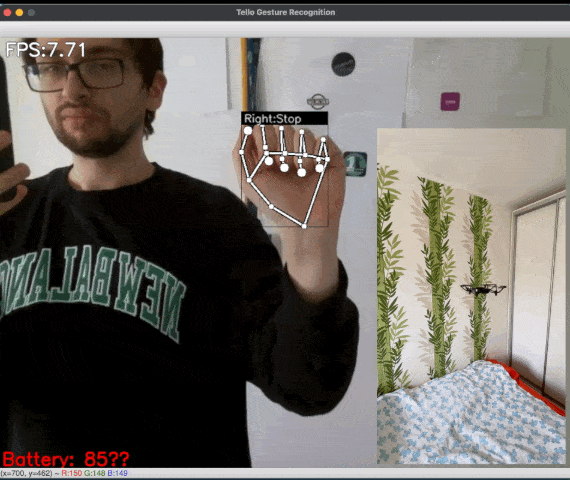
Figure 1: [GIF] Demonstration of drone flight control via gestures using MediaPipe Hands

Why use gesture recognition?

Gestures are the most natural way for people to express information in a non-verbal way. Gesture control is an entire topic in computer science that aims to interpret human gestures using algorithms. Users can simply control devices or interact without physically touching them. Nowadays, such types of control can be found from smart TV to surgery robots, and UAVs are not the exception.

Although gesture control for drones have not been widely explored lately, the approach has some advantages:

No additional equipment needed.
More human-friendly controls.
All you need is a camera that is already on all drones.

With all these features, such a control method has many applications.

Flying action camera. In extreme sports, drones are a trendy video recording tool. However, they tend to have a very cumbersome control panel. The ability to use basic gestures to control the drone (while in action) without reaching for the remote control would make it easier to use the drone as a selfie camera. And the ability to customise gestures would completely cover all the necessary actions.

This type of control as an alternative would be helpful in an industrial environment like, for example, construction conditions when there may be several drone operators (gesture can be used as a stop-signal in case of losing primary source of control).

The Emergencies and Rescue Services could use this system for mini-drones indoors or in hard-to-reach places where one of the hands is busy. Together with the obstacle avoidance system, this would make the drone fully autonomous, but still manageable when needed without additional equipment.

Another area of application is FPV (first-person view) drones. Here the camera on the headset could be used instead of one on the drone to recognise gestures. Because hand movement can be impressively precise, this type of control, together with hand position in space, can simplify the FPV drone control principles for new users.

However, all these applications need a reliable and fast (really fast) recognition system. Existing gesture recognition systems can be fundamentally divided into two main categories: first - where special physical devices are used, such as smart gloves or other on-body sensors; second - visual recognition using various types of cameras. Most of those solutions need additional hardware or rely on classical computer vision techniques. Hence, that is the fast solution, but it's pretty hard to add custom gestures or even motion ones. The answer we found is MediaPipe Hands that was used for this project.

Overall project structure

To create the proof of concept for the stated idea, a Ryze Tello quadcopter was used as a UAV. This drone has an open Python SDK, which greatly simplified the development of the program. However, it also has technical limitations that do not allow it to run gesture recognition on the drone itself (yet). For this purpose a regular PC or Mac was used. The video stream from the drone and commands to the drone are transmitted via regular WiFi, so no additional equipment was needed.

To make the program structure as plain as possible and add the opportunity for easily adding gestures, the program architecture is modular, with a control module and a gesture recognition module.

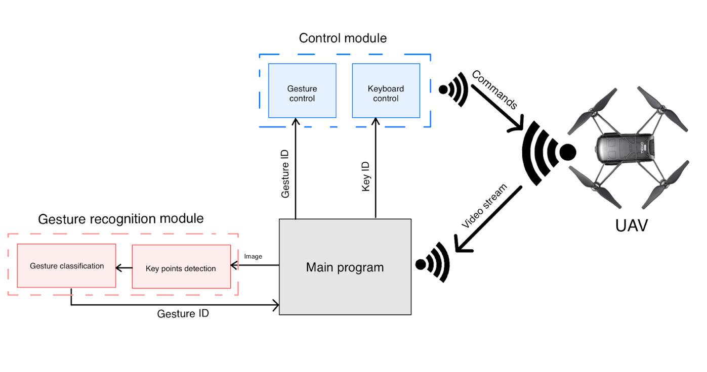
Figure 2: Scheme that shows overall project structure and how videostream data from the drone is processed

The application is divided into two main parts: gesture recognition and drone controller. Those are independent instances that can be easily modified. For example, to add new gestures or change the movement speed of the drone.

Video stream is passed to the main program, which is a simple script with module initialisation, connections, and typical for the hardware while-true cycle. Frame for the videostream is passed to the gesture recognition module. After getting the ID of the recognised gesture, it is passed to the control module, where the command is sent to the UAV. Alternatively, the user can control a drone from the keyboard in a more classical manner.

So, you can see that the gesture recognition module is divided into keypoint detection and gesture classifier. Exactly the bunch of the MediaPipe key point detector along with the custom gesture classification model distinguishes this gesture recognition system from most others.

Gesture recognition with MediaPipe

Utilizing MediaPipe Hands is a winning strategy not only in terms of speed, but also in flexibility. MediaPipe already has a simple gesture recognition calculator that can be inserted into the pipeline. However, we needed a more powerful solution with the ability to quickly change the structure and behaviour of the recognizer. To do so and classify gestures, the custom neural network was created with 4 Fully-Connected layers and 1 Softmax layer for classification.

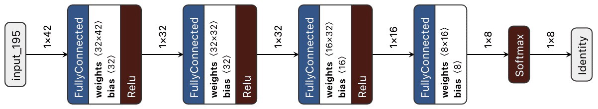
Figure 3: Scheme that shows the structure of classification neural network

This simple structure gets a vector of 2D coordinates as an input and gives the ID of the classified gesture.

Instead of using cumbersome segmentation models with a more algorithmic recognition process, a simple neural network can easily handle such tasks. Recognising gestures by keypoints, which is a simple vector with 21 points` coordinates, takes much less data and time. What is more critical, new gestures can be easily added because model retraining tasks take much less time than the algorithmic approach.

To train the classification model, dataset with keypoints` normalised coordinates and ID of a gesture was used. The numerical characteristic of the dataset was that:

3 gestures with 300+ examples (basic gestures)
5 gestures with 40 -150 examples

All data is a vector of x, y coordinates that contain small tilt and different shapes of hand during data collection.

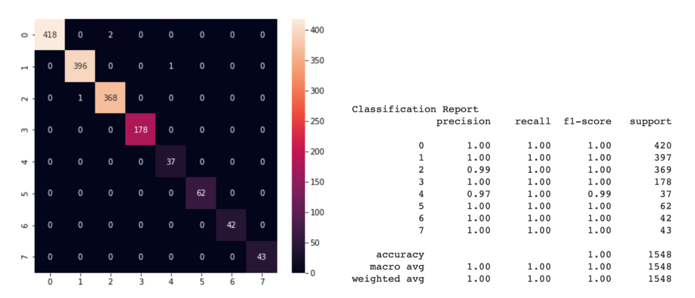
Figure 4: Confusion matrix and classification report for classification

We can see from the classification report that the precision of the model on the test dataset (this is 30% of all data) demonstrated almost error-free for most classes, precision > 97% for any class. Due to the simple structure of the model, excellent accuracy can be obtained with a small number of examples for training each class. After conducting several experiments, it turned out that we just needed the dataset with less than 100 new examples for good recognition of new gestures. What is more important, we don’t need to retrain the model for each motion in different illumination because MediaPipe takes over all the detection work.

Figure 5: [GIF] Test that demonstrates how fast classification network can distinguish newly trained gestures using the information from MediaPipe hand detector

From gestures to movements

To control a drone, each gesture should represent a command for a drone. Well, the most excellent part about Tello is that it has a ready-made Python API to help us do that without explicitly controlling motors hardware. We just need to set each gesture ID to a command.

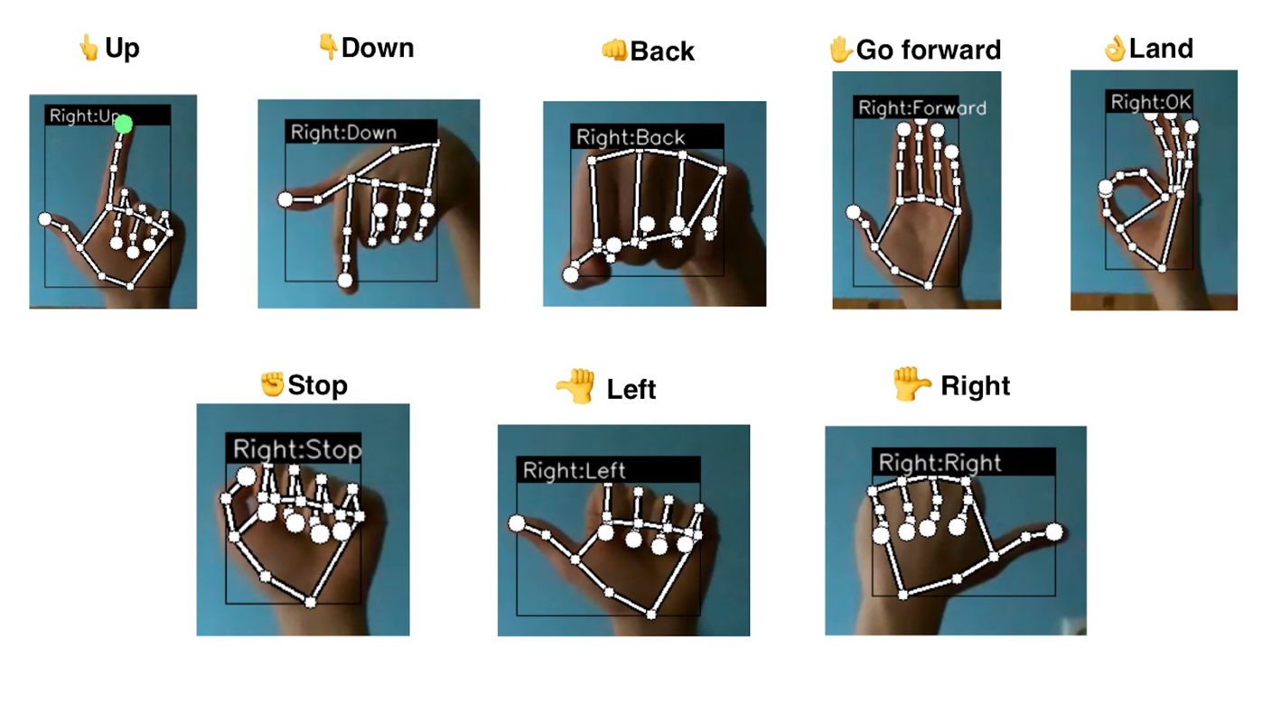
Figure 6: Command-gesture pairs representation

Each gesture sets the speed for one of the axes; that’s why the drone’s movement is smooth, without jitter. To remove unnecessary movements due to false detection, even with such a precise model, a special buffer was created, which is saving the last N gestures. This helps to remove glitches or inconsistent recognition.

The fundamental goal of this project is to demonstrate the superiority of the keypoint-based gesture recognition approach compared to classical methods. To demonstrate all the potential of this recognition model and its flexibility, there is an ability to create the dataset on the fly … on the drone`s flight! You can create your own combinations of gestures or rewrite an existing one without collecting massive datasets or manually setting a recognition algorithm. By pressing the button and ID key, the vector of detected points is instantly saved to the overall dataset. This new dataset can be used to retrain classification network to add new gestures for the detection. For now, there is a notebook that can be run on Google Colab or locally. Retraining the network-classifier takes about 1-2 minutes on a standard CPU instance. The new binary file of the model can be used instead of the old one. It is as simple as that. But for the future, there is a plan to do retraining right on the mobile device or even on the drone.

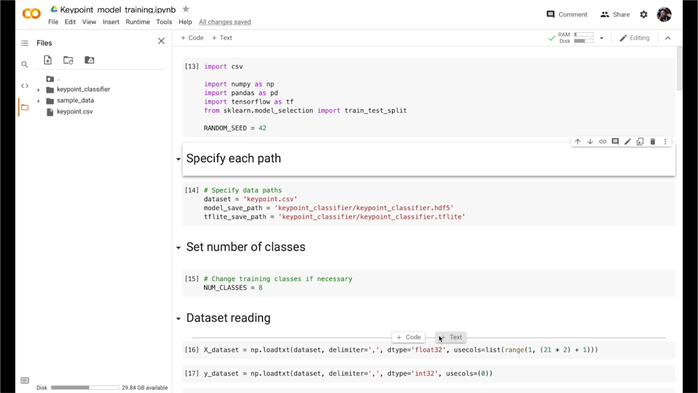
Figure 7: Notebook for model retraining in action

Summary

This project is created to make a push in the area of the gesture-controlled drones. The novelty of the approach lies in the ability to add new gestures or change old ones quickly. This is made possible thanks to MediaPipe Hands. It works incredibly fast, reliably, and ready out of the box, making gesture recognition very fast and flexible to changes. Our Neuron Lab`s team is excited about the demonstrated results and going to try other incredible solutions that MediaPipe provides.

We will also keep track of MediaPipe updates, especially about adding more flexibility in creating custom calculators for our own models and reducing barriers to entry when creating them. Since at the moment our classifier model is outside the graph, such improvements would make it possible to quickly implement a custom calculator with our model into reality.

Another highly anticipated feature is Flutter support (especially for iOS). In the original plans, the inference and visualisation were supposed to be on a smartphone with NPU\GPU utilisation, but at the moment support quality does not satisfy our requests. Flutter is a very powerful tool for rapid prototyping and concept checking. It allows us to throw and test an idea cross-platform without involving a dedicated mobile developer, so such support is highly demanded.

Nevertheless, the development of this demo project continues with available functionality, and there are already several plans for the future. Like using the MediaPipe Holistic for face recognition and subsequent authorisation. The drone will be able to authorise the operator and give permission for gesture control. It also opens the way to personalisation. Since the classifier network is straightforward, each user will be able to customise gestures for themselves (simply by using another version of the classifier model). Depending on the authorised user, one or another saved model will be applied. Also in the plans to add the usage of Z-axis. For example, tilt the palm of your hand to control the speed of movement or height more precisely. We encourage developers to innovate responsibly in this area, and to consider responsible AI practices such as testing for unfair biases and designing with safety and privacy in mind.

We highly believe that this project will motivate even small teams to do projects in the field of ML computer vision for the UAV, and MediaPipe will help to cope with the limitations and difficulties on their way (such as scalability, cross-platform support and GPU inference).

If you want to contribute, have ideas or comments about this project, please reach out to [email protected], or visit the GitHub page of the project.

This blog post is curated by Igor Kibalchich, ML Research Product Manager at Google AI.

Source: Google Developers Blog

Drone control via gestures using MediaPipe Hands

A guest post by Neurons Lab

Please note that the information, uses, and applications expressed in the below post are solely those of our guest author, Neurons Lab, and not necessarily those of Google.

How the idea emerged

Figure 1: [GIF] Demonstration of drone flight control via gestures using MediaPipe Hands

Why use gesture recognition?

Although gesture control for drones have not been widely explored lately, the approach has some advantages:

No additional equipment needed.
More human-friendly controls.
All you need is a camera that is already on all drones.

With all these features, such a control method has many applications.

Overall project structure

To make the program structure as plain as possible and add the opportunity for easily adding gestures, the program architecture is modular, with a control module and a gesture recognition module.

Figure 2: Scheme that shows overall project structure and how videostream data from the drone is processed

Gesture recognition with MediaPipe

Figure 3: Scheme that shows the structure of classification neural network

This simple structure gets a vector of 2D coordinates as an input and gives the ID of the classified gesture.

To train the classification model, dataset with keypoints` normalised coordinates and ID of a gesture was used. The numerical characteristic of the dataset was that:

3 gestures with 300+ examples (basic gestures)
5 gestures with 40 -150 examples

All data is a vector of x, y coordinates that contain small tilt and different shapes of hand during data collection.

Figure 4: Confusion matrix and classification report for classification

Figure 5: [GIF] Test that demonstrates how fast classification network can distinguish newly trained gestures using the information from MediaPipe hand detector

From gestures to movements

Figure 6: Command-gesture pairs representation

Figure 7: Notebook for model retraining in action

Summary

If you want to contribute, have ideas or comments about this project, please reach out to [email protected], or visit the GitHub page of the project.

This blog post is curated by Igor Kibalchich, ML Research Product Manager at Google AI.

Source: Google Developers Blog

Discovering Anomalous Data with Self-Supervised Learning

Posted by Kihyuk Sohn and Chun-Liang Li, Research Scientists, Google Cloud

Anomaly detection (sometimes called outlier detection or out-of-distribution detection) is one of the most common machine learning applications across many domains, from defect detection in manufacturing to fraudulent transaction detection in finance. It is most often used when it is easy to collect a large amount of known-normal examples but where anomalous data is rare and difficult to find. As such, one-class classification, such as one-class support vector machine (OC-SVM) or support vector data description (SVDD), is particularly relevant to anomaly detection because it assumes the training data are all normal examples, and aims to identify whether an example belongs to the same distribution as the training data. Unfortunately, these classical algorithms do not benefit from the representation learning that makes machine learning so powerful. On the other hand, substantial progress has been made in learning visual representations from unlabeled data via self-supervised learning, including rotation prediction and contrastive learning. As such, combining one-class classifiers with these recent successes in deep representation learning is an under-explored opportunity for the detection of anomalous data.

In “Learning and Evaluating Representations for Deep One-class Classification”, presented at ICLR 2021, we outline a 2-stage framework that makes use of recent progress on self-supervised representation learning and classic one-class algorithms. The algorithm is simple to train and results in state-of-the-art performance on various benchmarks, including CIFAR, f-MNIST, Cat vs Dog and CelebA. We then follow up on this in “CutPaste: Self-Supervised Learning for Anomaly Detection and Localization”, presented at CVPR 2021, in which we propose a new representation learning algorithm under the same framework for a realistic industrial defect detection problem. The framework achieves a new state-of-the-art on the MVTec benchmark.

A Two-Stage Framework for Deep One-Class Classification
While end-to-end learning has demonstrated success in many machine learning problems, including deep learning algorithm designs, such an approach for deep one-class classifiers often suffer from degeneration in which the model outputs the same results regardless of the input.

To combat this, we apply a two stage framework. In the first stage, the model learns deep representations with self-supervision. In the second stage, we adopt one-class classification algorithms, such as OC-SVM or kernel density estimator, using the learned representations from the first stage. This 2-stage algorithm is not only robust to degeneration, but also enables one to build more accurate one-class classifiers. Furthermore, the framework is not limited to specific representation learning and one-class classification algorithms — that is, one can easily plug-and-play different algorithms, which is useful if any advanced approaches are developed.

A deep neural network is trained to generate the representations of input images via self-supervision. We then train one-class classifiers on the learned representations.

Semantic Anomaly Detection
We test the efficacy of our 2-stage framework for anomaly detection by experimenting with two representative self-supervised representation learning algorithms, rotation prediction and contrastive learning.

Rotation prediction refers to a model’s ability to predict the rotated angles of an input image. Due to its promising performance in other computer vision applications, the end-to-end trained rotation prediction network has been widely adopted for one-class classification research. The existing approach typically reuses the built-in rotation prediction classifier for learning representations to conduct anomaly detection, which is suboptimal because those built-in classifiers are not trained for one-class classification.

In contrastive learning, a model learns to pull together representations from transformed versions of the same image, while pushing representations of different images away. During training, as images are drawn from the dataset, each is transformed twice with simple augmentations (e.g., random cropping or color changing). We minimize the distance of the representations from the same image to encourage consistency and maximize the distance between different images. However, usual contrastive learning converges to a solution where all the representations of normal examples are uniformly spread out on a sphere. This is problematic because most of the one-class algorithms determine the outliers by checking the proximity of a tested example to the normal training examples, but when all the normal examples are uniformly distributed in an entire space, outliers will always appear close to some normal examples.

To resolve this, we propose distribution augmentation (DA) for one-class contrastive learning. The idea is that instead of learning representations from the training data only, the model learns from the union of the training data plus augmented training examples, where the augmented examples are considered to be different from the original training data. We employ geometric transformations, such as rotation or horizontal flip, for distribution augmentation. With DA, the training data is no longer uniformly distributed in the representation space because some areas are occupied by the augmented data.

Left: Illustrated examples of perfect uniformity from the standard contrastive learning. Right: The reduced uniformity by the proposed distribution augmentation (DA), where the augmented data occupy the space to avoid the uniform distribution of the inlier examples (blue) throughout the whole sphere.

We evaluate the performance of one-class classification in terms of the area under receiver operating characteristic curve (AUC) on the commonly used datasets in computer vision, including CIFAR10 and CIFAR-100, Fashion MNIST, and Cat vs Dog. Images from one class are given as inliers and those from remaining classes are given as outliers. For example, we see how well cat images are detected as anomalies when dog images are inliers.

	CIFAR-10	CIFAR-100	f-MNIST	Cat v.s. Dog
Ruff et al. (2018)	64.8	-	-	-
Golan and El-Yaniv (2018)	86.0	78.7	93.5	88.8
Bergman and Hoshen (2020)	88.2	-	94.1	-
Hendrycks et al. (2019)	90.1	-	-	-
Huang et al. (2019)	86.6	78.8	93.9	-
2-stage framework: rotation prediction	91.3±0.3	84.1±0.6	95.8±0.3	86.4±0.6
2-stage framework: contrastive (DA)	92.5±0.6	86.5±0.7	94.8±0.3	89.6±0.5

Performance comparison of one-class classification methods. Values are the mean AUCs and their standard deviation over 5 runs. AUC ranges from 0 to 100, where 100 is perfect detection.

Given the suboptimal built-in rotation prediction classifiers typically used for rotation prediction approaches, it’s notable that simply replacing the built-in rotation classifier used in the first stage for learning representations with a one-class classifier at the second stage of the proposed framework significantly boosts the performance, from 86 to 91.3 AUC. More generally, the 2-stage framework achieves state-of-the-art performance on all of the above benchmarks.

With classic OC-SVM, which learns the area boundary of representations of normal examples, the 2-stage framework results in higher performance than existing works as measured by image-level AUC.

Texture Anomaly Detection for Industrial Defect Detection
In many real-world applications of anomaly detection, the anomaly is often defined by localized defects instead of entirely different semantics (i.e., being different in general). For example, the detection of texture anomalies is useful for detecting various kinds of industrial defects.

The examples of semantic anomaly detection and defect detection. In semantic anomaly detection, the inlier and outlier are different in general, (e.g., one is a dog, the other a cat). In defect detection, the semantics for inlier and outlier are the same (e.g., they are both tiles), but the outlier has a local anomaly.

While learning representations with rotation prediction and distribution-augmented contrastive learning have demonstrated state-of-the-art performance on semantic anomaly detection, those algorithms do not perform well on texture anomaly detection. Instead, we explored different representation learning algorithms that better fit the application.

In our second paper, we propose a new self-supervised learning algorithm for texture anomaly detection. The overall anomaly detection follows the 2-stage framework, but the first stage, in which the model learns deep image representations, is specifically trained to predict whether the image is augmented via a simple CutPaste data augmentation. The idea of CutPaste augmentation is simple — a given image is augmented by randomly cutting a local patch and pasting it back to a different location of the same image. Learning to distinguish normal examples from CutPaste-augmented examples encourages representations to be sensitive to local irregularity of an image.

The illustration of learning representations by predicting CutPaste augmentations. Given an example, the CutPaste augmentation crops a local patch, then pasties it to a randomly selected area of the same image. We then train a binary classifier to distinguish the original image and the CutPaste augmented image.

We use MVTec, a real-world defect detection dataset with 15 object categories, to evaluate the approach above.

DOCC (Ruff et al., 2020)	U-Student (Bergmann et al., 2020)	Rotation Prediction	Contrastive (DA)	CutPaste
87.9	92.5	86.3	86.5	95.2

Image-level anomaly detection performance (in AUC) on the MVTec benchmark.

Besides image-level anomaly detection, we use the CutPaste method to locate where the anomaly is, i.e., “patch-level” anomaly detection. We aggregate the patch anomaly scores via upsampling with Gaussian smoothing and visualize them in heatmaps that show where the anomaly is. Interestingly, this provides decently improved localization of anomalies. The below table shows the pixel-level AUC for localization evaluation.

Autoencoder (Bergmann et al., 2019)	FCDD (Ruff et al., 2020)	Rotation Prediction	Contrastive (DA)	CutPaste
86.0	92.0	93.0	90.4	96.0

Pixel-level anomaly localization performance (in AUC) comparison between different algorithms on the MVTec benchmark.

Conclusion
In this work we introduce a novel 2-stage deep one-class classification framework and emphasize the importance of decoupling building classifiers from learning representations so that the classifier can be consistent with the target task, one-class classification. Moreover, this approach permits applications of various self-supervised representation learning methods, attaining state-of-the-art performance on various applications of visual one-class classification from semantic anomaly to texture defect detection. We are extending our efforts to build more realistic anomaly detection methods under the scenario where training data is truly unlabeled.

Acknowledgements
We gratefully acknowledge the contribution from other co-authors, including Jinsung Yoon, Minho Jin and Tomas Pfister. We release the code in our GitHub repository.

Source: Google AI Blog

Machine Learning GDEs: Q2 ‘21 highlights and achievements

Posted by HyeJung Lee, MJ You, ML Ecosystem Community Managers

Google Developers Experts (GDE) is a community of passionate developers who love to share their knowledge with others. Many of them specialize in Machine Learning (ML).

Here are some highlights showcasing the ML GDEs achievements from last quarter, which contributed to the global ML ecosystem. If you are interested in becoming an ML GDE, please scroll down to see how you can apply!

ML Developers meetup @Google I/O

At I/O this year, we held two ML Developers Meetups (America/APAC and EMEA/APAC). Merve Noyan/Yusuf Sarıgöz (Turkey), Sayak Paul/Bhavesh Bhatt (India), Leigh Johnson/Margaret Maynard-Reid (USA), David Cardozo (Columbia), Vinicius Caridá/Arnaldo Gualberto (Brazil) shared their experiences in developing ML products with TensorFlow, Cloud AI or JAX and also introduced projects they are currently working on.

I/O Extended 2021

Chart showing what's included in Vertex AI

After I/O, many ML GDEs posted recap summaries of the I/O on their blogs. Chansung Park (Korea) outlined the ML keynote summary, while US-based Victor Dibia wrapped up the Top 10 Machine Learning and Design Insights from Google IO 2021.

Vertex AI was the topic of conversation at the event. Minori Matsuda from Japan wrote a Japanese article titled “Introduction of powerful Vertex AI AutoML Forecasting.” Similarly, Piero Esposito (Brazil) posted an article titled “Serverless Machine Learning Pipelines with Vertex AI: An Introduction,” including a tutorial on fully customized code. India-based Sayak Paul co-authored a blog post discussing key pieces in Vertex AI right after the Vertex AI announcement showing how to run a TensorFlow training job using Vertex AI.

Communities such as Google Developers Groups (GDG) and TensorFlow User Groups (TFUG) held extended events where speakers further discussed different ML topics from I/O, including China-based Song Lin’s presentation on TensorFlow highlights and Applications experiences from I/O which had 24,000 online attendees. Chansung Park (Korea) also gave a presentation on what Vertex AI is and what you can do with Vertex AI.

Cloud AI

Leigh Johnson (USA) wrote an article titled Soft-launching an AI/ML Product as a Solo Founder, covering GCP AutoML Vision, GCP IoT Core, TensorFlow Model Garden, and TensorFlow.js. The article details the journey of a solo founder developing an ML product for detecting printing failure for 3D printers (more on this story is coming up soon, so stay tuned!)

Demo and code examples from Victor Dibia (USA)’s New York Taxi project, Minori Matsuda (Japan)’s article on AutoML and AI Platform notebook, Srivatsan Srinivasan (USA)’s video tutorials, Sayak Paul (India)’s Distributed Training in TensorFlow with AI Platform & Docker and Chansung Park (Korea)’s curated personal newsletter were all published together on Cloud blog.

Aqsa Kausar (Pakistan) gave a talk about Explainable AI in Google Cloud at the International Women’s Day Philippines event. She explained why it is important and where and how it is applied in ML workflows.

Finally, ML Lab by Robert John from Nigeria, introduces the ML landscape on GCP covering from BigQueryML through AutoML to TensorFlow and AI Platform.

TensorFlow

Eliyar Eziz (China) published a book “TensorFlow 2 with real-life use cases”. Gant Laborde from the US authored book “Learning TensorFlow.js” which is published by O'Reilly and wrote an article “No Data No Problem - TensorFlow.js Transfer Learning” about seeking out new datasets to boldly train where no models have trained before. He also published “A Riddikulus Dataset” which talks about creating the Harry Potter dataset.

Hong Kong-based Guan Wang published a research paper, “Iterated Dilated Convolutional Neural Networks for Word Segmentation,” covering state-of-the-art performance improvement, which is implemented on TensorFlow by Keras.

Elyes Manai from Tunisia wrote an article “Become a Tensorflow Certified Developer ” - a guide to TensorFlow Certificate and tips.

Greece-based George Soloupis wrote a tutorial “Fine-tune a BERT model with the use of Colab TPU” on how to finetune a BERT model that was trained specifically on greek language to perform the downstream task of text classification, using Colab’s TPU (v2–8).

JAX

India-based Aakash Nain has published the TF-JAX tutorial series (Part1, Part2, Part3, Part 4), aiming to teach everyone the building blocks of TensorFlow and JAX frameworks.

Online Meetup TensorFlow and JAX by Tzer-jen Wei from Taiwan covered JAX intro and use cases. It also touched upon different ways of writing TensorFlow models and training loops.

YouTube video Neural Networks, with a practical example written in JAX, probably the first JAX techtalk in Portuguese by João Guilherme Madeia Araújo (Brazil).

Keras

A lot of Keras examples were contributed by Sayak Paul from India and listed below are some of these examples.

Semi-supervision and domain adaptation with AdaMatch (github) covering implementation and walkthrough of AdaMatch (SOTA in unsupervised domain adaptation)
Learning to Resize in Computer Vision (github)
Keypoint Detection with Transfer Learning (github)

Kaggle

Notebook “Simple Bayesian Ridge with Sentence Embeddings” by Ertuğrul Demir (Turkey) about a natural language processing task using BERT finetuning followed by simple linear regression on top of sentence embeddings generated by transformers.

Youhan Lee from Korea gave a talk about “Learning machine learning and TensorFlow with Kaggle competition”. He explained how to use the Kaggle platform for learning ML.

Research

Advances in machine learning and deep learning research are changing our technology, and many ML GDEs are interested and contributing.

Learning Neurl Compositional Neural Programs for Continuous Control

Karim Beguir (UK) co-authored a paper with the DeepMind team covering a novel compositional approach using Deep Reinforcement Learning to solve robotics manipulation tasks. The paper was accepted in the NeurIPS workshop.

Finally, Sayak Paul from India, together with Pin-Yu Chen, published a research paper, “Vision Transformers are Robust Learners,” covering the robustness of the Vision Transformer (ViT) against common corruptions and perturbations, distribution shifts, and natural adversarial examples.

If you want to know more about the Google Experts community and their global open-source ML contributions, please check the GDE Program website, visit the GDE Directory and connect with GDEs on Twitter and LinkedIn. You can also meet them virtually on the ML GDE’s YouTube Channel!

Source: Google Developers Blog

Improved Detection of Elusive Polyps via Machine Learning

Posted by Yossi Matias, Vice President and Ehud Rivlin, Research Scientist, Google Research

With the increasing ability to consistently and accurately process large amounts of data, particularly visual data, computer-aided diagnostic systems are more frequently being used to assist physicians in their work. This, in turn, can lead to meaningful improvements in health care. An example of where this could be especially useful is in the diagnosis and treatment of colorectal cancer (CRC), which is especially deadly and results in over 900K deaths per year, globally. CRC originates in small pre-cancerous lesions in the colon, called polyps, the identification and removal of which is very successful in preventing CRC-related deaths.

The standard procedure used by gastroenterologists (GIs) to detect and remove polyps is the colonoscopy, and about 19 million such procedures are performed annually in the US alone. During a colonoscopy, the gastroenterologist uses a camera-containing probe to check the intestine for pre-cancerous polyps and early signs of cancer, and removes tissue that looks worrisome. However, complicating factors, such as incomplete detection (in which the polyp appears within the field of view, but is missed by the GI, perhaps due to its size or shape) and incomplete exploration (in which the polyp does not appear in the camera’s field of view), can lead to a high fraction of missed polyps. In fact, studies suggest that 22%–28% of polyps are missed during colonoscopies, of which 20%–24% have the potential to become cancerous (adenomas).

Today, we are sharing progress made in using machine learning (ML) to help GIs fight colorectal cancer by making colonoscopies more effective. In “Detection of Elusive Polyps via a Large Scale AI System”, we present an ML model designed to combat the problem of incomplete detection by helping the GI detect polyps that are within the field of view. This work adds to our previously published work that maximizes the coverage of the colon during the colonoscopy by flagging for GI follow-up areas that may have been missed. Using clinical studies, we show that these systems significantly improve polyp detection rates.

Incomplete Exploration
To help the GI detect polyps that are outside the field of view, we previously developed an ML system that reduces the rate of incomplete exploration by estimating the fractions of covered and non-covered regions of a colon during a colonoscopy. This earlier work uses computer vision and geometry in a technique we call colonoscopy coverage deficiency via depth, to compute segment-by-segment coverage for the colon. It does so in two phases: first computing depth maps for each frame of the colonoscopy video, and then using these depth maps to compute the coverage in real time.

The ML system computes a depth image (middle) from a single RGB image (left). Then, based on the computation of depth images for a video sequence, it calculates local coverage (right), and detects where the coverage has been deficient and a second look is required (blue color indicates observed segments where red indicates uncovered ones). You can learn more about this work in our previous blog post.

This segment-by-segment work yields the ability to estimate what fraction of the current segment has been covered. The helpfulness of such functionality is clear: during the procedure itself, a physician may be alerted to segments with deficient coverage, and can immediately return to review these areas, potentially reducing the rates of missed polyps due to incomplete exploration.

Incomplete Detection
In our most recent paper, we look into the problem of incomplete detection. We describe an ML model that aids a GI in detecting polyps that are within the field of view, so as to reduce the rate of incomplete detection. We developed a system that is based on convolutional neural networks (CNN) with an architecture that combines temporal logic with a single frame detector, resulting in more accurate detection.

This new system has two principal advantages. The first is that the system improves detection performance by reducing the number of false negatives detections of elusive polyps, those polyps that are particularly difficult for GIs to detect. The second advantage is the very low false positive rate of the system. This low false positive rate makes these systems more likely to be adopted in the clinic.

Examples of the variety of polyps detected by the ML system.

We trained the system on 3600 procedures (86M video frames) and tested it on 1400 procedures (33M frames). All the videos and metadata were de-identified. The system detected 97% of the polyps (i.e., it yielded 97% sensitivity) at 4.6 false alarms per procedure, which is a substantial improvement over previously published results. Of the false alarms, follow-up review showed that some were, in fact, valid polyp detections, indicating that the system was able to detect polyps that were missed by the performing endoscopist and by those who annotated the data. The performance of the system on these elusive polyps suggests its generalizability in that the system has learned to detect examples that were initially missed by all who viewed the procedure.

We evaluated the system performance on polyps that are in the field of view for less than five seconds, which makes them more difficult for the GI to detect, and for which models typically have much lower sensitivity. In this case the system attained a sensitivity that is about three times that of the sensitivity that the original procedure achieved. When the polyps were present in the field of view for less than 2 seconds, the difference was even more stark — the system exhibited a 4x improvement in sensitivity.

It is also interesting to note that the system is fairly insensitive to the choice of neural network architecture. We used two architectures: RetinaNet and LSTM-SSD. RetinaNet is a leading technique for object detection on static images (used for video by applying it to frames in a consecutive fashion). It is one of the top performers on a variety of benchmarks, given a fixed computational budget, and is known for balancing speed of computation with accuracy. LSTM-SSD is a true video object detection architecture, which can explicitly account for the temporal character of the video (e.g., temporal consistency of detections, ability to deal with blur and fast motion, etc.). It is known for being robust and very computationally lightweight and can therefore run on less expensive processors. Comparable results were also obtained on the much heavier Faster R-CNN architecture. The fact that results are similar across different architectures implies that one can choose the network meeting the available hardware specifications.

Prospective Clinical Research Study
As part of the research reported in our detection paper we ran a clinical validation on 100 procedures in collaboration with Shaare Zedek Medical Center in Jerusalem, where our system was used in real time to help GIs. The system helped detect an average of one polyp per procedure that would have otherwise been missed by the GI performing the procedure, while not missing any of the polyps detected by the GIs, and with 3.8 false alarms per procedure. The feedback from the GIs was consistently positive.

We are encouraged by the potential helpfulness of this system for improving polyp detection, and we look forward to working together with the doctors in the procedure room to further validate this research.

Acknowledgements
The research was conducted by teams from Google Health and Google Research, Israel with support from Verily Life Sciences, and in collaboration with Shaare Zedek Medical Center. Verily is advancing this research via a newly established center in Israel, led by Ehud Rivlin. This research was conducted by Danny Veikherman, Tomer Golany, Dan M. Livovsky, Amit Aides, Valentin Dashinsky, Nadav Rabani, David Ben Shimol, Yochai Blau, Liran Katzir, Ilan Shimshoni, Yun Liu, Ori Segol, Eran Goldin, Greg Corrado, Jesse Lachter, Yossi Matias, Ehud Rivlin, and Daniel Freedman. Our appreciation also goes to several institutions and GIs who provided advice along the way and tested our system prototype. We would like to thank all of our team members and collaborators who worked on this project with us, including: Chen Barshai, Nia Stoykova, and many others.

Source: Google AI Blog

Improved Detection of Elusive Polyps via Machine Learning

Posted by Yossi Matias, Vice President and Ehud Rivlin, Research Scientist, Google Research

Examples of the variety of polyps detected by the ML system.

Source: Google AI Blog

High Fidelity Image Generation Using Diffusion Models

Posted by Jonathan Ho, Research Scientist and Chitwan Saharia, Software Engineer, Google Research, Brain Team

Natural image synthesis is a broad class of machine learning (ML) tasks with wide-ranging applications that pose a number of design challenges. One example is image super-resolution, in which a model is trained to transform a low resolution image into a detailed high resolution image (e.g., RAISR). Super-resolution has many applications that can range from restoring old family portraits to improving medical imaging systems. Another such image synthesis task is class-conditional image generation, in which a model is trained to generate a sample image from an input class label. The resulting generated sample images can be used to improve performance of downstream models for image classification, segmentation, and more.

Generally, these image synthesis tasks are performed by deep generative models, such as GANs, VAEs, and autoregressive models. Yet each of these generative models has its downsides when trained to synthesize high quality samples on difficult, high resolution datasets. For example, GANs often suffer from unstable training and mode collapse, and autoregressive models typically suffer from slow synthesis speed.

Alternatively, diffusion models, originally proposed in 2015, have seen a recent revival in interest due to their training stability and their promising sample quality results on image and audio generation. Thus, they offer potentially favorable trade-offs compared to other types of deep generative models. Diffusion models work by corrupting the training data by progressively adding Gaussian noise, slowly wiping out details in the data until it becomes pure noise, and then training a neural network to reverse this corruption process. Running this reversed corruption process synthesizes data from pure noise by gradually denoising it until a clean sample is produced. This synthesis procedure can be interpreted as an optimization algorithm that follows the gradient of the data density to produce likely samples.

Today we present two connected approaches that push the boundaries of the image synthesis quality for diffusion models — Super-Resolution via Repeated Refinements (SR3) and a model for class-conditioned synthesis, called Cascaded Diffusion Models (CDM). We show that by scaling up diffusion models and with carefully selected data augmentation techniques, we can outperform existing approaches. Specifically, SR3 attains strong image super-resolution results that surpass GANs in human evaluations. CDM generates high fidelity ImageNet samples that surpass BigGAN-deep and VQ-VAE2 on both FID score and Classification Accuracy Score by a large margin.

SR3: Image Super-Resolution
SR3 is a super-resolution diffusion model that takes as input a low-resolution image, and builds a corresponding high resolution image from pure noise. The model is trained on an image corruption process in which noise is progressively added to a high-resolution image until only pure noise remains. It then learns to reverse this process, beginning from pure noise and progressively removing noise to reach a target distribution through the guidance of the input low-resolution image..

With large scale training, SR3 achieves strong benchmark results on the super-resolution task for face and natural images when scaling to resolutions 4x–8x that of the input low-resolution image. These super-resolution models can further be cascaded together to increase the effective super-resolution scale factor, e.g., stacking a 64x64 → 256x256 and a 256x256 → 1024x1024 face super-resolution model together in order to perform a 64x64 → 1024x1024 super-resolution task.

We compare SR3 with existing methods using human evaluation study. We conduct a Two-Alternative Forced Choice Experiment where subjects are asked to choose between the reference high resolution image, and the model output when asked the question, “Which image would you guess is from a camera?” We measure the performance of the model through confusion rates (% of time raters choose the model outputs over reference images, where a perfect algorithm would achieve a 50% confusion rate). The results of this study are shown in the figure below.

Above: We achieve close to 50% confusion rate on the task of 16x16 → 128x128 faces, outperforming state-of-the-art face super-resolution methods PULSE and FSRGAN. Below: We also achieve a 40% confusion rate on the much more difficult task of 64x64 → 256x256 natural images, outperforming the regression baseline by a large margin.

CDM: Class-Conditional ImageNet Generation
Having shown the effectiveness of SR3 in performing natural image super-resolution, we go a step further and use these SR3 models for class-conditional image generation. CDM is a class-conditional diffusion model trained on ImageNet data to generate high-resolution natural images. Since ImageNet is a difficult, high-entropy dataset, we built CDM as a cascade of multiple diffusion models. This cascade approach involves chaining together multiple generative models over several spatial resolutions: one diffusion model that generates data at a low resolution, followed by a sequence of SR3 super-resolution diffusion models that gradually increase the resolution of the generated image to the highest resolution. It is well known that cascading improves quality and training speed for high resolution data, as shown by previous studies (for example in autoregressive models and VQ-VAE-2) and in concurrent work for diffusion models. As demonstrated by our quantitative results below, CDM further highlights the effectiveness of cascading in diffusion models for sample quality and usefulness in downstream tasks, such as image classification.

Example of the cascading pipeline that includes a sequence of diffusion models: the first generates a low resolution image, and the rest perform upsampling to the final high resolution image. Here the pipeline is for class-conditional ImageNet generation, which begins with a class-conditional diffusion model at 32x32 resolution, followed by 2x and 4x class-conditional super-resolution using SR3.

Selected generated images from our 256x256 cascaded class-conditional ImageNet model.

Along with including the SR3 model in the cascading pipeline, we also introduce a new data augmentation technique, which we call conditioning augmentation, that further improves the sample quality results of CDM. While the super-resolution models in CDM are trained on original images from the dataset, during generation they need to perform super-resolution on the images generated by a low-resolution base model, which may not be of sufficiently high quality in comparison to the original images. This leads to a train-test mismatch for the super-resolution models. Conditioning augmentation refers to applying data augmentation to the low-resolution input image of each super-resolution model in the cascading pipeline. These augmentations, which in our case include Gaussian noise and Gaussian blur, prevents each super-resolution model from overfitting to its lower resolution conditioning input, eventually leading to better higher resolution sample quality for CDM.

Altogether, CDM generates high fidelity samples superior to BigGAN-deep and VQ-VAE-2 in terms of both FID score and Classification Accuracy Score on class-conditional ImageNet generation. CDM is a pure generative model that does not use a classifier to boost sample quality, unlike other models such as ADM and VQ-VAE-2. See below for quantitative results on sample quality.

Class-conditional ImageNet FID scores at the 256x256 resolution for methods that do not use extra classifiers to boost sample quality. BigGAN-deep is reported at its best truncation value. (Lower is better.)

ImageNet classification accuracy scores at the 256x256 resolution, measuring the validation set accuracy of a classifier trained on generated data. CDM generated data attains significant gains over existing methods, closing the gap in classification accuracy between real and generated data. (Higher is better.)

Conclusion
With SR3 and CDM, we have pushed the performance of diffusion models to state-of-the-art on super-resolution and class-conditional ImageNet generation benchmarks. We are excited to further test the limits of diffusion models for a wide variety of generative modeling problems. For more information on our work, please visit Image Super-Resolution via Iterative Refinement and Cascaded Diffusion Models for High Fidelity Image Generation.

Acknowledgements:
We thank our co-authors William Chan, Mohammad Norouzi, Tim Salimans, and David Fleet, and we are grateful for research discussions and assistance from Ben Poole, Jascha Sohl-Dickstein, Doug Eck, and the rest of the Google Research, Brain Team. Thanks to Tom Small for helping us with the animations.

Source: Google AI Blog

Announcing Android’s updateable, fully integrated ML inference stack

Posted by Oli Gaymond, Product Manager, Android ML

On-Device Machine Learning provides lower latency, more efficient battery usage, and features that do not require network connectivity. We have found that development teams deploying on-device ML on Android today encounter these common challenges:

Many apps are size constrained, so having to bundle and manage additional libraries just for ML can be a significant cost
Unlike server-based ML, the compute environment is highly heterogeneous, resulting in significant differences in performance, stability and accuracy
Maximising reach can lead to using older more broadly available APIs; which limits usage of the latest advances in ML.

To help solve these problems, we’ve built Android ML Platform - an updateable, fully integrated ML inference stack. With Android ML Platform, developers get:

Built in on-device inference essentials - we will provide on-device inference binaries with Android and keep them up to date; this reduces apk size
Optimal performance on all devices - we will optimize the integration with Android to automatically make performance decisions based on the device, including enabling hardware acceleration when available
A consistent API that spans Android versions - regular updates are delivered via Google Play Services and are made available outside of the Android OS release cycle

Built in on-device inference essentials - TensorFlow Lite for Android

TensorFlow Lite will be available on all devices with Google Play Services. Developers will no longer need to include the runtime in their apps, reducing app size. Moreover, TensorFlow Lite for Android will use metadata in the model to automatically enable hardware acceleration, allowing developers to get the best performance possible on each Android device.

Optimal performance on all devices - Automatic Acceleration

Automatic Acceleration is a new feature in TensorFlowLite for Android. It enables per-model testing to create allowlists for specific devices taking performance, accuracy and stability into account. These allowlists can be used at runtime to decide when to turn on hardware acceleration. In order to use accelerator allowlisting, developers will need to provide additional metadata to verify correctness. Automatic Acceleration will be available later this year.

A consistent API that spans Android versions

Besides keeping TensorFlow Lite for Android up to date via regular updates, we’re also going to be updating the Neural Networks API outside of OS releases while keeping the API specification the same across Android versions. In addition we are working with chipset vendors to provide the latest drivers for their hardware directly to devices, outside of OS updates. This will let developers dramatically reduce testing from thousands of devices to a handful of configurations. We’re excited to announce that we’ll be launching later this year with Qualcomm as our first partner.

Sign-up for our early access program

While several of these features will roll out later this year, we are providing early access to TensorFlow Lite for Android to developers who are interested in getting started sooner. You can sign-up for our early access program here.

Source: Android Developers Blog

Quickly Training Game-Playing Agents with Machine Learning

Posted by Leopold Haller and Hernan Moraldo, Software Engineers, Google Research

In the last two decades, dramatic advances in compute and connectivity have allowed game developers to create works of ever-increasing scope and complexity. Simple linear levels have evolved into photorealistic open worlds, procedural algorithms have enabled games with unprecedented variety, and expanding internet access has transformed games into dynamic online services. Unfortunately, scope and complexity have grown more rapidly than the size of quality assurance teams or the capabilities of traditional automated testing. This poses a challenge to both product quality (such as delayed releases and post-launch patches) and developer quality of life.

Machine learning (ML) techniques offer a possible solution, as they have demonstrated the potential to profoundly impact game development flows – they can help designers balance their game and empower artists to produce high-quality assets in a fraction of the time traditionally required. Furthermore, they can be used to train challenging opponents that can compete at the highest levels of play. Yet some ML techniques can pose requirements that currently make them impractical for production game teams, including the design of game-specific network architectures, the development of expertise in implementing ML algorithms, or the generation of billions of frames of training data. Conversely, game developers operate in a setting that offers unique advantages to leverage ML techniques, such as direct access to the game source, an abundance of expert demonstrations, and the uniquely interactive nature of video games.

Today, we present a ML-based system that game developers can use to quickly and efficiently train game-testing agents, helping developers find serious bugs quickly while allowing human testers to focus on more complex and intricate problems. The resulting solution requires no ML expertise, works on many of the most popular game genres, and can train an ML policy, which generates game actions from game state, in less than an hour on a single game instance. We have also released an open source library that demonstrates a functional application of these techniques.

Supported genres include arcade, action/adventure, and racing games.

The Right Tool for the Right Job
The most elemental form of video game testing is to simply play the game. A lot. Many of the most serious bugs (such as crashes or falling out of the world) are easy to detect and fix; the challenge is finding them within the vast state space of a modern game. As such, we decided to focus on training a system that could “just play the game” at scale.

We found that the most effective way to do this was not to try to train a single, super effective agent that could play the entire game from end-to-end, but to provide developers with the ability to train an ensemble of game-testing agents, each of which could effectively accomplish tasks of a few minutes each, which game developers refer to as “gameplay loops”.

These core gameplay behaviors are often expensive to program through traditional means, but are much more efficient to train than a single end-to-end ML model. In practice, commercial games create longer loops by repeating and remixing core gameplay loops, which means that developers can test large stretches of gameplay by combining ML policies with a small amount of simple scripting.

Simulation-centric, Semantic API
One of the most fundamental challenges in applying ML to game development is bridging the chasm between the simulation-centric world of video games and the data-centric world of ML. Rather than ask developers to directly convert the game state into custom, low-level ML features (which would be too labor intensive) or attempting to learn from raw pixels (which would require too much data to train), our system provides developers with an idiomatic, game-developer friendly API that allows them to describe their game in terms of the essential state that a player observes and the semantic actions they can perform. All of this information is expressed via concepts that are familiar to game developers, such as entities, raycasts, 3D positions and rotations, buttons and joysticks.

As you can see in the example below, the API allows the specification of observations and actions in just a few lines of code.

Example actions and observations for a racing game.

From API to Neural Network
This high level, semantic API is not just easy to use but also allows the system to flexibly adapt to the specific game being developed – the specific combination of API building blocks employed by the game developer informs our choice of network architecture, since it provides information about the type of gaming scenario in which the system is deployed. Some examples of this include: handling action outputs differently depending on whether they represent a digital button or analog joystick, or using techniques from image processing to handle observations that result from an agent probing its environment with raycasts (similar to how autonomous vehicles probe their environment with LIDAR).

Our API is sufficiently general to allow modeling of many common control-schemes (the configuration of action outputs that control movement) in games, such as first-person games, third-person games with camera-relative controls, racing games, twin stick shooters, etc. Since 3D movement and aiming are often an integral aspect of gameplay in general, we create networks that automatically tend towards simple behaviors such as aiming, approach or avoidance in these games. The system accomplishes this by analyzing the game’s control scheme to create neural network layers that perform custom processing of observations and actions in that game. For example, positions and rotations of objects in the world are automatically translated into directions and distances from the point of view of the AI-controlled game entity. This transformation typically increases the speed of learning and helps the learned network generalize better.

An example neural network generated for a game with joystick controls and raycast inputs. Depending on the inputs (red) and the control scheme, the system generates custom pre- and post-processing layers (orange).

Learning From The Experts in Real Time
After generating a neural network architecture, the network needs to be trained to play the game using an appropriate choice of learning algorithm.

Reinforcement learning (RL), in which an ML policy is trained directly to maximize a reward, may seem like the obvious choice since they have been successfully used to train highly competent ML policies for games. However, RL algorithms tend to require more data than a single game instance can produce in a reasonable amount of time, and achieving good results in a new domain often requires hyperparameter tuning and strong ML domain knowledge.

Instead, we found that imitation learning (IL), which trains ML policies based by observing experts play the game, works well for our use case. Unlike RL, where the agent needs to discover a good policy on its own, IL only needs to recreate the behavior of a human expert. Since game developers and testers are experts in their own games, they can easily provide demonstrations of how to play the game.

We use an IL approach inspired by the DAgger algorithm, which allows us to take advantage of video games’ most compelling quality – interactivity. Thanks to the reductions in training time and data requirements enabled by our semantic API, training is effectively realtime, giving a developer the ability to fluidly switch between providing gameplay demonstrations and watching the system play. This results in a natural feedback loop, in which a developer iteratively provides corrections to a continuous stream of ML policies.

From the developer’s perspective, providing a demonstration or a correction to faulty behavior is as simple as picking up the controller and starting to play the game. Once they are done, they can put the controller down and watch the ML policy play. The result is a training experience that is real-time, interactive, highly experiential, and, very often, more than a little fun.

ML policy for an FPS game, trained with our system.

Conclusion
We present a system which combines a high-level semantic API with a DAgger-inspired interactive training flow that enables training of useful ML policies for video game testing in a wide variety of genres. We have released an open source library as a functional illustration of our system. No ML expertise is required and training of agents for test applications often takes less than an hour on a single developer machine. We hope that this work will help inspire the development of ML techniques that can be deployed in real-world game-development flows in ways that are accessible, effective, and fun to use.

Acknowledgements
We’d like to thank the core members of the project: Dexter Allen, Leopold Haller, Nathan Martz, Hernan Moraldo, Stewart Miles and Hina Sakazaki. Training algorithms are provided by TF Agents, and on-device inference by TF Lite. Special thanks to our research advisors, Olivier Bachem, Erik Frey, and Toby Pohlen, and to Eugene Brevdo, Jared Duke, Oscar Ramirez and Neal Wu who provided helpful guidance and support.

Source: Google AI Blog

Developer updates from Coral

Posted by The Coral Team

We're always excited to share updates to our Coral platform for building edge ML applications. In this post, we have some interesting demos, interfaces, and tutorials to share, and we'll start by pointing you to an important software update for the Coral Dev Board.

Important update for the Dev Board / SoM

If you have a Coral Dev Board or Coral SoM, please install our latest Mendel update as soon as possible to receive a critical fix to part of the SoC power configuration. To get it, just log onto your board and install the update as follows:

This will install a patch from NXP for the Dev Board / SoM's SoC, without which it's possible the SoC will overstress and the lifetime of the device could be reduced. If you recently flashed your board with the latest system image, you might already have this fix (we also updated the flashable image today), but it never hurts to fetch all updates, as shown above.

Note: This update does not apply to the Dev Board Mini.

Manufacturing demo

We recently published the Coral Manufacturing Demo, which demonstrates how to use a single Coral Edge TPU to simultaneously accomplish two common manufacturing use-cases: worker safety and visual inspection.

The demo is designed for two specific videos and tasks (worker keepout detection and apple quality grading) but it is designed to be easily customized with different inputs and tasks. The demo, written in C++, requires OpenGL and is primarily targeted at x86 systems which are prevalent in manufacturing gateways – although ARM Cortex-A systems, like the Coral Dev Board, are also supported.

Web Coral

We've been working hard to make ML acceleration with the Coral Edge TPU available for most popular systems. So we're proud to announce support for WebUSB, allowing you to use the Coral USB Accelerator directly from Chrome. To get started, check out our WebCoral demo, which builds a webpage where you can select a model and run an inference accelerated by the Edge TPU.

New models repository

We recently released a new models repository that makes it easier to explore the various trained models available for the Coral platform, including image classification, object detection, semantic segmentation, pose estimation, and speech recognition. Each family page lists the various models, including details about training dataset, input size, latency, accuracy, model size, and other parameters, making it easier to select the best fit for the application at hand. Lastly, each family page includes links to training scripts and example code to help you get started. Or for an overview of all our models, you can see them all on one page.

Models, trained TensorFlow models for the Edge TPU

Transfer learning tutorials

Even with our collection of pre-trained models, it can sometimes be tricky to create a task-specific model that's compatible with our Edge TPU accelerator. To make this easier, we've released some new Google Colab tutorials that allow you to perform transfer learning for object detection, using MobileDet and EfficientDet-Lite models. You can find these and other Colabs in our GitHub Tutorials repo.

We are excited to share all that Coral has to offer as we continue to evolve our platform. Keep an eye out for more software and platform related news coming this summer. To discover more about our edge ML platform, please visit Coral.ai and share your feedback at [email protected].