Author Archives: Google AI

Improved Detection of Elusive Polyps via Machine Learning

With the increasing ability to consistently and accurately process large amounts of data, particularly visual data, computer-aided diagnostic systems are more frequently being used to assist physicians in their work. This, in turn, can lead to meaningful improvements in health care. An example of where this could be especially useful is in the diagnosis and treatment of colorectal cancer (CRC), which is especially deadly and results in over 900K deaths per year, globally. CRC originates in small pre-cancerous lesions in the colon, called polyps, the identification and removal of which is very successful in preventing CRC-related deaths.

The standard procedure used by gastroenterologists (GIs) to detect and remove polyps is the colonoscopy, and about 19 million such procedures are performed annually in the US alone. During a colonoscopy, the gastroenterologist uses a camera-containing probe to check the intestine for pre-cancerous polyps and early signs of cancer, and removes tissue that looks worrisome. However, complicating factors, such as incomplete detection (in which the polyp appears within the field of view, but is missed by the GI, perhaps due to its size or shape) and incomplete exploration (in which the polyp does not appear in the camera’s field of view), can lead to a high fraction of missed polyps. In fact, studies suggest that 22%–28% of polyps are missed during colonoscopies, of which 20%–24% have the potential to become cancerous (adenomas).

Today, we are sharing progress made in using machine learning (ML) to help GIs fight colorectal cancer by making colonoscopies more effective. In “Detection of Elusive Polyps via a Large Scale AI System”, we present an ML model designed to combat the problem of incomplete detection by helping the GI detect polyps that are within the field of view. This work adds to our previously published work that maximizes the coverage of the colon during the colonoscopy by flagging for GI follow-up areas that may have been missed. Using clinical studies, we show that these systems significantly improve polyp detection rates.

Incomplete Exploration
To help the GI detect polyps that are outside the field of view, we previously developed an ML system that reduces the rate of incomplete exploration by estimating the fractions of covered and non-covered regions of a colon during a colonoscopy. This earlier work uses computer vision and geometry in a technique we call colonoscopy coverage deficiency via depth, to compute segment-by-segment coverage for the colon. It does so in two phases: first computing depth maps for each frame of the colonoscopy video, and then using these depth maps to compute the coverage in real time.

The ML system computes a depth image (middle) from a single RGB image (left). Then, based on the computation of depth images for a video sequence, it calculates local coverage (right), and detects where the coverage has been deficient and a second look is required (blue color indicates observed segments where red indicates uncovered ones). You can learn more about this work in our previous blog post.

This segment-by-segment work yields the ability to estimate what fraction of the current segment has been covered. The helpfulness of such functionality is clear: during the procedure itself, a physician may be alerted to segments with deficient coverage, and can immediately return to review these areas, potentially reducing the rates of missed polyps due to incomplete exploration.

Incomplete Detection
In our most recent paper, we look into the problem of incomplete detection. We describe an ML model that aids a GI in detecting polyps that are within the field of view, so as to reduce the rate of incomplete detection. We developed a system that is based on convolutional neural networks (CNN) with an architecture that combines temporal logic with a single frame detector, resulting in more accurate detection.

This new system has two principal advantages. The first is that the system improves detection performance by reducing the number of false negatives detections of elusive polyps, those polyps that are particularly difficult for GIs to detect. The second advantage is the very low false positive rate of the system. This low false positive rate makes these systems more likely to be adopted in the clinic.

Examples of the variety of polyps detected by the ML system.

We trained the system on 3600 procedures (86M video frames) and tested it on 1400 procedures (33M frames). All the videos and metadata were de-identified. The system detected 97% of the polyps (i.e., it yielded 97% sensitivity) at 4.6 false alarms per procedure, which is a substantial improvement over previously published results. Of the false alarms, follow-up review showed that some were, in fact, valid polyp detections, indicating that the system was able to detect polyps that were missed by the performing endoscopist and by those who annotated the data. The performance of the system on these elusive polyps suggests its generalizability in that the system has learned to detect examples that were initially missed by all who viewed the procedure.

We evaluated the system performance on polyps that are in the field of view for less than five seconds, which makes them more difficult for the GI to detect, and for which models typically have much lower sensitivity. In this case the system attained a sensitivity that is about three times that of the sensitivity that the original procedure achieved. When the polyps were present in the field of view for less than 2 seconds, the difference was even more stark — the system exhibited a 4x improvement in sensitivity.

It is also interesting to note that the system is fairly insensitive to the choice of neural network architecture. We used two architectures: RetinaNet and  LSTM-SSD. RetinaNet is a leading technique for object detection on static images (used for video by applying it to frames in a consecutive fashion). It is one of the top performers on a variety of benchmarks, given a fixed computational budget, and is known for balancing speed of computation with accuracy. LSTM-SSD is a true video object detection architecture, which can explicitly account for the temporal character of the video (e.g., temporal consistency of detections, ability to deal with blur and fast motion, etc.). It is known for being robust and very computationally lightweight and can therefore run on less expensive processors. Comparable results were also obtained on the much heavier Faster R-CNN architecture. The fact that results are similar across different architectures implies that one can choose the network meeting the available hardware specifications.

Prospective Clinical Research Study
As part of the research reported in our detection paper we ran a clinical validation on 100 procedures in collaboration with Shaare Zedek Medical Center in Jerusalem, where our system was used in real time to help GIs. The system helped detect an average of one polyp per procedure that would have otherwise been missed by the GI performing the procedure, while not missing any of the polyps detected by the GIs, and with 3.8 false alarms per procedure. The feedback from the GIs was consistently positive.

We are encouraged by the potential helpfulness of this system for improving polyp detection, and we look forward to working together with the doctors in the procedure room to further validate this research.

Acknowledgements
The research was conducted by teams from Google Health and Google Research, Israel with support from Verily Life Sciences, and in collaboration with Shaare Zedek Medical Center. Verily is advancing this research via a newly established center in Israel, led by Ehud Rivlin. This research was conducted by Danny Veikherman, Tomer Golany, Dan M. Livovsky, Amit Aides, Valentin Dashinsky, Nadav Rabani, David Ben Shimol, Yochai Blau, Liran Katzir, Ilan Shimshoni, Yun Liu, Ori Segol, Eran Goldin, Greg Corrado, Jesse Lachter, Yossi Matias, Ehud Rivlin, and Daniel Freedman. Our appreciation also goes to several institutions and GIs who provided advice along the way and tested our system prototype. We would like to thank all of our team members and collaborators who worked on this project with us, including: Chen Barshai, Nia Stoykova, and many others.
Source: Google AI Blog


Improved Detection of Elusive Polyps via Machine Learning

With the increasing ability to consistently and accurately process large amounts of data, particularly visual data, computer-aided diagnostic systems are more frequently being used to assist physicians in their work. This, in turn, can lead to meaningful improvements in health care. An example of where this could be especially useful is in the diagnosis and treatment of colorectal cancer (CRC), which is especially deadly and results in over 900K deaths per year, globally. CRC originates in small pre-cancerous lesions in the colon, called polyps, the identification and removal of which is very successful in preventing CRC-related deaths.

The standard procedure used by gastroenterologists (GIs) to detect and remove polyps is the colonoscopy, and about 19 million such procedures are performed annually in the US alone. During a colonoscopy, the gastroenterologist uses a camera-containing probe to check the intestine for pre-cancerous polyps and early signs of cancer, and removes tissue that looks worrisome. However, complicating factors, such as incomplete detection (in which the polyp appears within the field of view, but is missed by the GI, perhaps due to its size or shape) and incomplete exploration (in which the polyp does not appear in the camera’s field of view), can lead to a high fraction of missed polyps. In fact, studies suggest that 22%–28% of polyps are missed during colonoscopies, of which 20%–24% have the potential to become cancerous (adenomas).

Today, we are sharing progress made in using machine learning (ML) to help GIs fight colorectal cancer by making colonoscopies more effective. In “Detection of Elusive Polyps via a Large Scale AI System”, we present an ML model designed to combat the problem of incomplete detection by helping the GI detect polyps that are within the field of view. This work adds to our previously published work that maximizes the coverage of the colon during the colonoscopy by flagging for GI follow-up areas that may have been missed. Using clinical studies, we show that these systems significantly improve polyp detection rates.

Incomplete Exploration
To help the GI detect polyps that are outside the field of view, we previously developed an ML system that reduces the rate of incomplete exploration by estimating the fractions of covered and non-covered regions of a colon during a colonoscopy. This earlier work uses computer vision and geometry in a technique we call colonoscopy coverage deficiency via depth, to compute segment-by-segment coverage for the colon. It does so in two phases: first computing depth maps for each frame of the colonoscopy video, and then using these depth maps to compute the coverage in real time.

The ML system computes a depth image (middle) from a single RGB image (left). Then, based on the computation of depth images for a video sequence, it calculates local coverage (right), and detects where the coverage has been deficient and a second look is required (blue color indicates observed segments where red indicates uncovered ones). You can learn more about this work in our previous blog post.

This segment-by-segment work yields the ability to estimate what fraction of the current segment has been covered. The helpfulness of such functionality is clear: during the procedure itself, a physician may be alerted to segments with deficient coverage, and can immediately return to review these areas, potentially reducing the rates of missed polyps due to incomplete exploration.

Incomplete Detection
In our most recent paper, we look into the problem of incomplete detection. We describe an ML model that aids a GI in detecting polyps that are within the field of view, so as to reduce the rate of incomplete detection. We developed a system that is based on convolutional neural networks (CNN) with an architecture that combines temporal logic with a single frame detector, resulting in more accurate detection.

This new system has two principal advantages. The first is that the system improves detection performance by reducing the number of false negatives detections of elusive polyps, those polyps that are particularly difficult for GIs to detect. The second advantage is the very low false positive rate of the system. This low false positive rate makes these systems more likely to be adopted in the clinic.

Examples of the variety of polyps detected by the ML system.

We trained the system on 3600 procedures (86M video frames) and tested it on 1400 procedures (33M frames). All the videos and metadata were de-identified. The system detected 97% of the polyps (i.e., it yielded 97% sensitivity) at 4.6 false alarms per procedure, which is a substantial improvement over previously published results. Of the false alarms, follow-up review showed that some were, in fact, valid polyp detections, indicating that the system was able to detect polyps that were missed by the performing endoscopist and by those who annotated the data. The performance of the system on these elusive polyps suggests its generalizability in that the system has learned to detect examples that were initially missed by all who viewed the procedure.

We evaluated the system performance on polyps that are in the field of view for less than five seconds, which makes them more difficult for the GI to detect, and for which models typically have much lower sensitivity. In this case the system attained a sensitivity that is about three times that of the sensitivity that the original procedure achieved. When the polyps were present in the field of view for less than 2 seconds, the difference was even more stark — the system exhibited a 4x improvement in sensitivity.

It is also interesting to note that the system is fairly insensitive to the choice of neural network architecture. We used two architectures: RetinaNet and  LSTM-SSD. RetinaNet is a leading technique for object detection on static images (used for video by applying it to frames in a consecutive fashion). It is one of the top performers on a variety of benchmarks, given a fixed computational budget, and is known for balancing speed of computation with accuracy. LSTM-SSD is a true video object detection architecture, which can explicitly account for the temporal character of the video (e.g., temporal consistency of detections, ability to deal with blur and fast motion, etc.). It is known for being robust and very computationally lightweight and can therefore run on less expensive processors. Comparable results were also obtained on the much heavier Faster R-CNN architecture. The fact that results are similar across different architectures implies that one can choose the network meeting the available hardware specifications.

Prospective Clinical Research Study
As part of the research reported in our detection paper we ran a clinical validation on 100 procedures in collaboration with Shaare Zedek Medical Center in Jerusalem, where our system was used in real time to help GIs. The system helped detect an average of one polyp per procedure that would have otherwise been missed by the GI performing the procedure, while not missing any of the polyps detected by the GIs, and with 3.8 false alarms per procedure. The feedback from the GIs was consistently positive.

We are encouraged by the potential helpfulness of this system for improving polyp detection, and we look forward to working together with the doctors in the procedure room to further validate this research.

Acknowledgements
The research was conducted by teams from Google Health and Google Research, Israel with support from Verily Life Sciences, and in collaboration with Shaare Zedek Medical Center. Verily is advancing this research via a newly established center in Israel, led by Ehud Rivlin. This research was conducted by Danny Veikherman, Tomer Golany, Dan M. Livovsky, Amit Aides, Valentin Dashinsky, Nadav Rabani, David Ben Shimol, Yochai Blau, Liran Katzir, Ilan Shimshoni, Yun Liu, Ori Segol, Eran Goldin, Greg Corrado, Jesse Lachter, Yossi Matias, Ehud Rivlin, and Daniel Freedman. Our appreciation also goes to several institutions and GIs who provided advice along the way and tested our system prototype. We would like to thank all of our team members and collaborators who worked on this project with us, including: Chen Barshai, Nia Stoykova, and many others.

Source: Google AI Blog


Two New Datasets for Conversational NLP: TimeDial and Disfl-QA

A key challenge in natural language processing (NLP) is building conversational agents that can understand and reason about different language phenomena that are unique to realistic speech. For example, because people do not always premeditate exactly what they are going to say, a natural conversation often includes interruptions to speech, called disfluencies. Such disfluencies can be simple (like interjections, repetitions, restarts, or corrections), which simply break the continuity of a sentence, or more complex semantic disfluencies, in which the underlying meaning of a phrase changes. In addition, understanding a conversation also often requires knowledge of temporal relationships, like whether an event precedes or follows another. However, conversational agents built on today’s NLP models often struggle when confronted with temporal relationships or with disfluencies, and progress on improving their performance has been slow. This is due, in part, to a lack of datasets that involve such interesting conversational and speech phenomena.

To stir interest in this direction within the research community, we are excited to introduce TimeDial, for temporal commonsense reasoning in dialog, and Disfl-QA, which focuses on contextual disfluencies. TimeDial presents a new multiple choice span filling task targeted for temporal understanding, with an annotated test set of over ~1.1k dialogs. Disfl-QA is the first dataset containing contextual disfluencies in an information seeking setting, namely question answering over Wikipedia passages, with ~12k human annotated disfluent questions. These benchmark datasets are the first of their kind and show a significant gap between human performance and current state of the art NLP models.

TimeDial
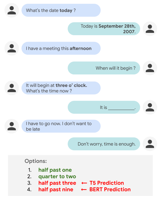
While people can effortlessly reason about everyday temporal concepts, such as duration, frequency, or relative ordering of events in a dialog, such tasks can be challenging for conversational agents. For example, current NLP models often make a poor selection when tasked with filling in a blank (as shown below) that assumes a basic level of world knowledge for reasoning, or that requires understanding explicit and implicit inter-dependencies between temporal concepts across conversational turns.

It is easy for a person to judge that “half past one” and “quarter to two” are more plausible options to fill in the blank than “half past three” and “half past nine”. However, performing such temporal reasoning in the context of a dialog is not trivial for NLP models, as it requires appealing to world knowledge (i.e., knowing that the participants are not yet late for the meeting) and understanding the temporal relationship between events (“half past one” is before “three o’clock”, while “half past three” is after it). Indeed, current state-of-the-art models like T5 and BERT end up picking the wrong answers — “half past three” (T5) and “half past nine” (BERT).

The TimeDial benchmark dataset (derived from the DailyDialog multi-turn dialog corpus) measures models’ temporal commonsense reasoning abilities within a dialog context. Each of the ~1.5k dialogs in the dataset is presented in a multiple choice setup, in which one temporal span is masked out and the model is asked to find all correct answers from a list of four options to fill in the blank.

In our experiments we found that while people can easily answer these multiple choice questions (at 97.8% accuracy), state-of-the-art pre-trained language models still struggle on this challenge set. We experiment across three different modeling paradigms: (i) classification over the provided 4 options using BERT, (ii) mask filling for the masked span in the dialog using BERT-MLM, (iii) generative methods using T5. We observe that all the models struggle on this challenge set, with the best variant only scoring 73%.

Model   2-best Accuracy
Human   97.8%
BERT - Classification   50.0%
BERT - Mask Filling   68.5%
T5 - Generation   73.0%

Qualitative error analyses show that the pre-trained language models often rely on shallow, spurious features (particularly text matching), instead of truly doing reasoning over the context. It is likely that building NLP models capable of performing the kind of temporal commonsense reasoning needed for TimeDial requires rethinking how temporal objects are represented within general text representations.

Disfl-QA
As disfluency is inherently a speech phenomenon, it is most commonly found in text output from speech recognition systems. Understanding such disfluent text is key to building conversational agents that understand human speech. Unfortunately, research in the NLP and speech community has been impeded by the lack of curated datasets containing such disfluencies, and the datasets that are available, like Switchboard, are limited in scale and complexity. As a result, it’s difficult to stress test NLP models in the presence of disfluencies.

Disfluency   Example
Interjection   When is, uh, Easter this year?
Repetition   When is EasEaster this year?
Correction   When is Lent, I mean Easter, this year?
Restart   How much, no wait, when is Easter this year?
Different kinds of disfluencies. The reparandum (words intended to be corrected or ignored; in red), interregnum (optional discourse cues; in grey) and repair (the corrected words; in blue).

Disfl-QA is the first dataset containing contextual disfluencies in an information seeking setting, namely question answering over Wikipedia passages from SQuAD. Disfl-QA is a targeted dataset for disfluencies, in which all questions (~12k) contain disfluencies, making for a much larger disfluent test set than prior datasets. Over 90% of the disfluencies in Disfl-QA are corrections or restarts, making it a much more difficult test set for disfluency correction. In addition, compared to earlier disfluency datasets, it contains a wider variety of semantic distractors, i.e., distractors that carry semantic meaning as opposed to simpler speech disfluencies. 

Passage: …The Normans (Norman: Nourmands; French: Normands; Latin: Normanni) were the people who in the 10th and 11th centuries gave their name to Normandy, a region in France. They were descended from Norse ("Norman" comes from "Norseman") raiders and pirates from Denmark, Iceland and Norway who, under their leader Rollo, …
Q1:   In what country is Normandy located? France ✓
DQ1:   In what country is Norse found no wait Normandy not Norse? Denmark X
Q2:   When were the Normans in Normandy? 10th and 11th centuries ✓
DQ2:   From which countries no tell me when were the Normans in Normandy? Denmark, Iceland and Norway X
A passage and questions (Qi) from SQuAD dataset, along with their disfluent versions (DQi), consisting of semantic distractors (like “Norse” and “from which countries”) and predictions from a T5 model.

Here, the first question (Q1) is seeking an answer about the location of Normandy. In the disfluent version (DQ1) Norse is mentioned before the question is corrected. The presence of this correctional disfluency confuses the QA model, which tends to rely on shallow textual cues from the question for making predictions.

Disfl-QA also includes newer phenomena, such as coreference (expression referring to the same entity) between the reparandum and the repair.

SQuAD  Disfl-QA
Who does BSkyB have an operating license from?  Who removed [BSkyB’s] operating license, no scratch that, who do [they] have [their] operating license from?

Experiments show that the performance of existing state-of-the-art language model–based question answering systems degrades significantly when tested on Disfl-QA and heuristic disfluencies (presented in the paper) in a zero-shot setting.

Dataset   F1
SQuAD   89.59
Heuristics   65.27 (-24.32)
Disfl-QA   61.64 (-27.95)

We show that data augmentation methods partially recover the loss in performance and also demonstrate the efficacy of using human-annotated training data for fine-tuning. We argue that researchers need large-scale disfluency datasets in order for NLP models to be robust to disfluencies.

Conclusion
Understanding language phenomena that are unique to human speech, like disfluencies and temporal reasoning, among others, is a key ingredient for enabling more natural human–machine communication in the near future. With TimeDial and Disfl-QA, we aim to fill a major research gap by providing these datasets as testbeds for NLP models, in order to evaluate their robustness to ubiquitous phenomena across different tasks. It is our hope that the broader NLP community will devise generalized few-shot or zero-shot approaches to effectively handle these phenomena, without requiring task-specific human-annotated training datasets, constructed specifically for these challenges.

Acknowledgments
The TimeDial work has been a team effort involving Lianhui Qi, Luheng He, Yenjin Choi, Manaal Faruqui and the authors. The Disfl-QA work has been a collaboration involving Jiacheng Xu, Diyi Yang, Manaal Faruqui.

Source: Google AI Blog


Google at ACL 2021

This week, the 59th annual meeting of the Association for Computational Linguistics (ACL), a premier conference covering a broad spectrum of research areas that are concerned with computational approaches to natural language, is taking place online.

As a leader in natural language processing and understanding, and a Diamond Level sponsor of ACL 2021, Google will showcase the latest research in the field with over 35 publications, and the organization of and participation in a variety of workshops and tutorials.

If you’re registered for ACL 2021, we hope that you’ll visit the Google virtual booth in Gather Town to learn more about the projects and opportunities at Google that go into solving interesting problems for billions of people. You can also learn more about Google's participation on the ACL 2021 Expo page, and see a full list of Google publications below (Google affiliations in bold).

Organizing Committee
Senior Area Chairs include: Dan Roth, Emily Pitler, Jimmy Lin, Ming-Wei Chang, Sebastian Ruder, Slav Petrov
Area Chairs include: Ankur P. Parikh, Artem Sokolov, Bhuwan Dhingra, Cicero Nogueira dos Santos, Colin Cherry, Dani Yogatama, David Mimno, Hideto Kazawa, Ian Tenney, Jasmijn Bastings, Jun Suzuki, Katja Filippova, Kyle Gorma, Lu Wang, Manaal Faruqui, Natalie Schluter, Peter Liu, Radu Soricut, Sebastian Gehrmann, Shashi Narayan, Tal Linzen, Vinodkumar Prabhakaran, Waleed Ammar

Publications
Parameter-Efficient Multi-task Fine-Tuning for Transformers via Shared Hypernetwork
Rabeeh Karimi Mahabadi*, Sebastian Ruder, Mostafa Dehghani, James Henderson

TicketTalk: Toward Human-Level Performance with End-to-End, Transaction-Based Dialog Systems
Bill Byrne, Karthik Krishnamoorthi, Saravanan Ganesh, Mihir Sanjay Kale

Increasing Faithfulness in Knowledge-Grounded Dialogue with Controllable Feature
Hannah Rashkin, David Reitter, Gaurav Singh Tomar, Dipanjan Das

Compositional Generalization and Natural Language Variation: Can a Semantic Parsing Approach Handle Both?
Peter Shaw, Ming-Wei Chang, Panupong Pasupat, Kristina Toutanova

Exploiting Language Relatedness for Low Web-Resource Language Model Adaptation: An Indic Languages Study
Yash Khemchandani, Sarvesh Mehtani, Vaidehi Patil, Abhijeet Awasthi, Partha Talukdar, Sunita Sarawagi

Causal Analysis of Syntactic Agreement Mechanisms in Neural Language Model
Matthew Finlayson, Aaron Mueller, Sebastian Gehrmann, Stuart Shieber, Tal Linzen*, Yonatan Belinkov

Modeling Fine-Grained Entity Types with Box Embeddings
Yasumasa Onoe, Michael Boratko, Andrew McCallum, Greg Durrett

TextSETTR: Few-Shot Text Style Extraction and Tunable Targeted Restyling
Parker Riley*, Noah Constant, Mandy Guo, Girish Kumar*, David Uthus, Zarana Parekh

Which Linguist Invented the Lightbulb? Presupposition Verification for Question-Answering
Najoung Kim*, Ellie Pavlick, Burcu Karagol Ayan, Deepak Ramachandran

H-Transformer-1D: Fast One-Dimensional Hierarchical Attention for Sequences
Zhenhai Zhu, Radu Soricut

Are Pretrained Convolutions Better than Pretrained Transformers?
Yi Tay, Mostafa Dehghani, Jai Gupta, Dara Bahri, Vamsi Aribandi, Zhen Qin, Donald Metzler

Benchmarking Scalable Methods for Streaming Cross Document Entity Coreference
Robert L Logan IV, Andrew McCallum, Sameer Singh, Dan Bikel

PhotoChat: A Human-Human Dialogue Dataset With Photo Sharing Behavior For Joint Image-Text Modeling
Xiaoxue Zang, Lijuan Liu, Maria Wang, Yang Song*, Hao Zhang, Jindong Chen

Focus Attention: Promoting Faithfulness and Diversity in Summarization
Rahul Aralikatte*, Shashi Narayan, Joshua Maynez, Sascha Rothe, Ryan McDonald*

A Cognitive Regularizer for Language Modeling
Jason Wei, Clara Meister, Ryan Cotterell

Language Model Augmented Relevance Score
Ruibo Liu, Jason Wei, Soroush Vosoughi

Cross-Replication Reliability - An Empirical Approach to Interpreting Inter-rater Reliability
Ka Wong, Praveen Paritosh, Lora Aroyo

TIMEDIAL: Temporal Commonsense Reasoning in Dialog
Lianhui Qin*, Aditya Gupta, Shyam Upadhyay, Luheng He, Yejin Choi, Manaal Faruqui

StructFormer: Joint Unsupervised Induction of Dependency and Constituency Structure from Masked Language Modeling
Yikang Shen*, Yi Tay, Che Zheng, Dara Bahri, Donald Metzler, Aaron Courville

MOLEMAN: Mention-Only Linking of Entities with a Mention Annotation Network
Nicholas FitzGerald, Jan A. Botha, Daniel Gillick, Daniel M. Bikel, Tom Kwiatkowski, Andrew McCallum

Neural Retrieval for Question Answering with Cross-Attention Supervised Data Augmentation
Yinfei Yanga, Ning Jinb, Kuo Linb, Mandy Guoa, Daniel Cera

ROPE: Reading Order Equivariant Positional Encoding for Graph-Based Document Information Extraction
Chen-Yu Lee, Chun-Liang Li, Chu Wang∗, Renshen Wang, Yasuhisa Fujii, Siyang Qin, Ashok Popat, Tomas Pfister

Measuring and Improving BERT’s Mathematical Abilities by Predicting the Order of Reasoning
Piotr Piekos, Henryk Michalewski, Mateusz Malinowsk

Improving Compositional Generalization in Classification Tasks via Structure Annotations
Juyong Kim, Pradeep Ravikumar, Joshua Ainslie, Santiago Ontañón

A Simple Recipe for Multilingual Grammatical Error Correction
Sascha Rothe, Jonathan Mallinson, Eric Malmi, Sebastian Krause, Aliaksei Severyn

nmT5 - Is Parallel Data Still Relevant for Pre-training Massively Multilingual Language Models?
Mihir Kale, Aditya Siddhant, Noah Constant, Melvin Johnson, Rami Al-Rfou, Linting Xue

QA-Driven Zero-Shot Slot Filling with Weak Supervision Pretraining
Xinya Du*, Luheng He, Qi Li, Dian Yu*, Panupong Pasupat, Yuan Zhang

AgreeSum: Agreement-Oriented Multi-Document Summarization
Richard Yuanzhe Pang*, Adam D. Lelkes, Vinh Q. Tran, Cong Yu

Disfl-QA: A Benchmark Dataset for Understanding Disfluencies in Question Answering
Aditya Gupta, Jiacheng Xu*, Shyam Upadhyay, Diyi Yang, Manaal Faruqui

Training ELECTRA Augmented with Multi-word Selection
Jiaming Shen*, Jialu Liu, Tianqi Liu, Cong Yu, Jiawei Han

A Survey of Data Augmentation Approaches for NLP
Steven Y. Feng, Varun Gangal, Jason Wei, Sarath Chandar, Soroush Vosoughi, Teruko Mitamura, Eduard Hovy

RealFormer: Transformer Likes Residual Attention
Ruining He, Anirudh Ravula, Bhargav Kanagal, Joshua Ainslie

Scaling Within Document Coreference to Long Texts
Raghuveer Thirukovalluru, Nicholas Monath, Kumar Shridhar, Manzil Zaheer, Mrinmaya Sachan, Andrew McCallum

MergeDistill: Merging Language Models using Pre-trained Distillation
Simran Khanuja, Melvin Johnson, Partha Talukdar

DoT: An Efficient Double Transformer for NLP tasks with Tables
Syrine Krichene, Thomas Müller*, Julian Martin Eisenschlos

How Reliable are Model Diagnostics?
Vamsi Aribandi, Yi Tay, Donald Metzler

Workshops
Interactive Learning for Natural Language Processing
Organizers include: Filip Radlinski
Invited Panelist: Julia Kreutzer

6th Workshop on Representation Learning for NLP (RepL4NLP-2021)
Organizers include: Chris Dyer, Laura Rimell

Third Workshop on Gender Bias for Natural Language Processing
Organizers include: Kellie Webster

Benchmarking: Past, Present and Future
Invited Speaker: Eunsol Choi

SemEval-2021, 15th International Workshop on Semantic Evaluation
Organizers include: Natalie Schluter

Workshop on Online Abuse and Harms
Organizers include: Vinodkumar Prabhakaran

GEM: Natural Language Generation, Evaluation, and Metrics
Organizers include: Sebastian Gehrmann

Workshop on Natural Language Processing for Programming
Invited Speaker: Charles Sutton

WPT 2021: The 17th International Conference on Parsing Technologies
Organizers include: Weiwei Sun

Tutorial
Recognizing Multimodal Entailment
Instructors include: Cesar Ilharco, Vaiva Imbrasaite, Ricardo Marino, Jannis Bulian, Chen Sun, Afsaneh Shirazi, Lucas Smaira, Cordelia Schmid


*  Work conducted while at Google. 

Source: Google AI Blog


Mapping Africa’s Buildings with Satellite Imagery

An accurate record of building footprints is important for a range of applications, from population estimation and urban planning to humanitarian response and environmental science. After a disaster, such as a flood or an earthquake, authorities need to estimate how many households have been affected. Ideally there would be up-to-date census information for this, but in practice such records may be out of date or unavailable. Instead, data on the locations and density of buildings can be a valuable alternative source of information.

A good way to collect such data is through satellite imagery, which can map the distribution of buildings across the world, particularly in areas that are isolated or difficult to access. However, detecting buildings with computer vision methods in some environments can be a challenging task. Because satellite imaging involves photographing the earth from several hundred kilometres above the ground, even at high resolution (30–50 cm per pixel), a small building or tent shelter occupies only a few pixels. The task is even more difficult for informal settlements, or rural areas where buildings constructed with natural materials can visually blend into the surroundings. There are also many types of natural and artificial features that can be easily confused with buildings in overhead imagery.

Objects that can confuse computer vision models for building identification (clockwise from top left) pools, rocks, enclosure walls and shipping containers.

In “Continental-Scale Building Detection from High-Resolution Satellite Imagery”, we address these challenges, using new methods for detecting buildings that work in rural and urban settings across different terrains, such as savannah, desert, and forest, as well as informal settlements and refugee facilities. We use this building detection model to create the Open Buildings dataset, a new open-access data resource containing the locations and footprints of 516 million buildings with coverage across most of the African continent. The dataset will support several practical, scientific and humanitarian applications, ranging from disaster response or population mapping to planning services such as new medical facilities or studying human impact on the natural environment.

Model Development
We built a training dataset for the building detection model by manually labelling 1.75 million buildings in 100k images. The figure below shows some examples of how we labelled images in the training data, taking into account confounding characteristics of different areas across the African continent. In rural areas, for example, it was necessary to identify different types of dwelling places and to disambiguate them from natural features, while in urban areas we needed to develop labelling policies for dense and contiguous structures.

(1) Example of a compound containing both dwelling places as well as smaller outbuildings such as grain stores. (2) Example of a round, thatched-roof structure that can be difficult for a model to distinguish from trees, and where it is necessary to use cues from pathways, clearings and shadows to disambiguate. (3) Example of several contiguous buildings for which the boundaries cannot be easily distinguished.

We trained the model to detect buildings in a bottom-up way, first by classifying each pixel as building or non-building, and then grouping these pixels together into individual instances. The detection pipeline was based on the U-Net model, which is commonly used in satellite image analysis. One advantage of U-Net is that it is a relatively compact architecture, and so can be applied to large quantities of imaging data without a heavy compute burden. This is critical, because the final task of applying this to continental-scale satellite imagery means running the model on many billions of image tiles.

Example of segmenting buildings in satellite imagery. Left: Source image; Center: Semantic segmentation, with each pixel assigned a confidence score that it is a building vs. non-building; Right: Instance segmentation, obtained by thresholding and grouping together connected components.

Initial experiments with the basic model had low precision and recall, for example due to the variety of natural and artificial features with building-like appearance. We found a number of methods that improved performance. One was the use of mixup as a regularisation method, where random training images are blended together by taking a weighted average. Though mixup was originally proposed for image classification, we modified it to be used for semantic segmentation. Regularisation is important in general for this building segmentation task, because even with 100k training images, the training data do not capture the full variation of terrain, atmospheric and lighting conditions that the model is presented with at test time, and hence, there is a tendency to overfit. This is mitigated by mixup as well as random augmentation of training images.

Another method that we found to be effective was the use of unsupervised self-training. We prepared a set of 100 million satellite images from across Africa, and filtered these to a subset of 8.7 million images that mostly contained buildings. This dataset was used for self-training using the Noisy Student method, in which the output of the best building detection model from the previous stage is used as a ‘teacher’ to then train a ‘student’ model that makes similar predictions from augmented images. In practice, we found that this reduced false positives and sharpened the detection output. The student model gave higher confidence to buildings and lower confidence to background.

Difference in model output between the student and teacher models for a typical image. In panel (d), red areas are those that the student model finds more likely to be buildings than the teacher model, and blue areas more likely to be background.

One problem that we faced initially was that our model had a tendency to create “blobby” detections, without clearly delineated edges and with a tendency for neighbouring buildings to be merged together. To address this, we applied another idea from the original U-Net paper, which is to use distance weighting to adapt the loss function to emphasise the importance of making correct predictions near boundaries. During training, distance weighting places greater emphasis at the edges by adding weight to the loss — particularly where there are instances that nearly touch. For building detection, this encourages the model to correctly identify the gaps in between buildings, which is important so that many close structures are not merged together. We found that the original U-Net distance weighting formulation was helpful but slow to compute. So, we developed an alternative based on Gaussian convolution of edges, which was both faster and more effective.

Distance weighting schemes to emphasise nearby edges: U-Net (left) and Gaussian convolution of edges (right).

Our technical report has more details on each of these methods.

Results
We evaluated the performance of the model on several different regions across the continent, in different categories: urban, rural, and medium-density. In addition, with the goal of preparing for potential humanitarian applications, we tested the model on regions with displaced persons and refugee settlements. Precision and recall did vary between regions, so achieving consistent performance across the continent is an ongoing challenge.

Precision-recall curves, measured at 0.5 intersection-over-union threshold.

When visually inspecting the detections for low-scoring regions, we noted various causes. In rural areas, label errors were problematic. For example, single buildings within a mostly-empty area can be difficult for labellers to spot. In urban areas, the model had a tendency to split large buildings into separate instances. The model also underperformed in desert terrain, where buildings were hard to distinguish against the background.

We carried out an ablation study to understand which methods contributed most to the final performance, measured in mean average precision (mAP). Distance weighting, mixup and the use of ImageNet pre-training were the biggest factors for the performance of the supervised learning baseline. The ablated models that did not use these methods had a mAP difference of -0.33, -0.12 and -0.07 respectively. Unsupervised self-training gave a further significant boost of +0.06 mAP.

Ablation study of training methods. The first row shows the mAP performance of the best model combined with self-training, and the second row shows the best model with supervised learning only (the baseline). By disabling each training optimization from the baseline in turn, we observe the impact on mAP test performance. Distance weighting has the most significant effect.

Generating the Open Buildings Dataset
To create the final dataset, we applied our best building detection model to satellite imagery across the African continent (8.6 billion image tiles covering 19.4 million km2, 64% of the continent), which resulted in the detection of 516M distinct structures.

Each building’s outline was simplified as a polygon and associated with a Plus Code, which is a geographic identifier made up of numbers and letters, akin to a street address, and useful for identifying buildings in areas that don’t have formal addressing systems. We also include confidence scores and guidance on suggested thresholds to achieve particular precision levels.

The sizes of the structures vary as shown below, tending towards small footprints. The inclusion of small structures is important, for example, to support analyses of informal settlements or refugee facilities.

Distribution of building footprint sizes.

The data is freely available and we look forward to hearing how it is used. In the future, we may add new features and regions, depending on usage and feedback.

Acknowledgements
This work is part of our AI for Social Good efforts and was led by Google Research, Ghana. Thanks to the co-authors of this work: Wojciech Sirko, Sergii Kashubin, Marvin Ritter, Abigail Annkah, Yasser Salah Edine Bouchareb, Yann Dauphin, Daniel Keysers, Maxim Neumann and Moustapha Cisse. We are grateful to Abdoulaye Diack, Sean Askay, Ruth Alcantara and Francisco Moneo for help with coordination. Rob Litzke, Brian Shucker, Yan Mayster and Michelina Pallone provided valuable assistance with geo infrastructure.

Source: Google AI Blog


Advances in TF-Ranking

In December 2018, we introduced TF-Ranking, an open-source TensorFlow-based library for developing scalable neural learning-to-rank (LTR) models, which are useful in settings where users expect to receive an ordered list of items in response to their query. LTR models — unlike standard classification models that classify one item at a time — receive an entire list of items as an input, and learn an ordering that maximizes the utility of the entire list. While search and recommendation systems are the most common applications of LTR models, since its release, we have seen TF-Ranking being applied in diverse domains beyond search, including e-commerce, SAT solvers, and smart city planning.

The goal of learning-to-rank (LTR) is to learn a function f() that takes as an input a list of items (documents, products, movies, etc.) and outputs the list of items in the optimal order (descending order of relevance). Here, green shade indicates item relevance level, and the red item marked with 'x' is non-relevant.

In May 2021, we published a major release of TF-Ranking that enables full support for natively building LTR models using Keras, a high-level API of TensorFlow 2. Our native Keras ranking model has a brand-new workflow design, including a flexible ModelBuilder, a DatasetBuilder to set up training data, and a Pipeline to train the model with the provided dataset. These components make building a customized LTR model easier than ever, and facilitate rapid exploration of new model structures for production and research. If RaggedTensors are your tool of choice, TF-Ranking is now working with them as well. In addition, our most recent release, which incorporates the Orbit training library, contains a long list of advances — the culmination of two and half years of neural LTR research. Below we share a few of the key improvements available in the latest TF-Ranking version.

Workflow to build and train a native Keras ranking model. Blue modules are provided by TF-Ranking, and green modules are customizable.

Learning-to-Rank with TFR-BERT
Recently, pretrained language models like BERT have achieved state-of-the-art performance on various language understanding tasks. To capture the expressiveness of these models, TF-Ranking implements a novel TFR-BERT architecture that couples BERT with the power of LTR to optimize the ordering of list inputs. As an example, consider a query and a list of n documents that one might like to rank in response to this query. Instead of learning an independent BERT representation for each <query, document> pair, LTR models apply a ranking loss to jointly learn a BERT representation that maximizes the utility of the entire ranked list with respect to the ground-truth labels.

The figure below illustrates this process. First, we flatten a list of n documents to rank in response to a query into a list <query, document> tuples. These tuples are fed into a pre-trained language model (e.g., BERT). The pooled BERT outputs for the entire document list are then jointly fine-tuned with one of the specialized ranking losses available in TF-Ranking. Our experience shows that this TFR-BERT architecture delivers significant improvements in pretrained language model performance, leading to state-of-the-art performance for several popular ranking tasks, especially when multiple pretrained language models are ensembled. Our users can now get started with TFR-BERT using this simple example.

An illustration of the TFR-BERT architecture, in which a joint LTR model over a list of n documents is constructed using BERT representations of individual <query, document> pairs.

Interpretable Learning-to-Rank
Transparency and interpretability are important factors in deploying LTR models in ranking systems that can be involved in determining the outcomes of processes such as loan eligibility assessment, advertisement targeting, or guiding medical treatment decisions. In such cases, the contribution of each individual feature to the final ranking should be examinable and understandable to ensure transparency, accountability and fairness of the outcomes.

One possible way to achieve this is using generalized additive models (GAMs) — intrinsically interpretable machine learning models that are linearly composed of smooth functions of individual features. However, while GAMs have been extensively studied on regression and classification tasks, it is less clear how to apply them in a ranking setting. For instance, while GAMs can be straightforwardly applied to model each individual item in the list, modeling both item interactions and the context in which these items are ranked is a more challenging research problem. To this end, we have developed a neural ranking GAM — an extension of generalized additive models to ranking problems.

Unlike standard GAMs, a neural ranking GAM can take into account both the features of the ranked items and the context features (e.g., query or user profile) to derive an interpretable, compact model. This ensures that not only the contribution of each item-level feature is interpretable, but also the contribution of the context features. For example, in the figure below, using a neural ranking GAM makes visible how distance, price, and relevance, in the context of a given user device, contribute to the final ranking of the hotel. Neural ranking GAMs are now available as a part of TF-Ranking,

An example of applying neural ranking GAM for local search. For each input feature (e.g., price, distance), a sub-model produces a sub-score that can be examined, providing transparency. Context features (e.g., user device type) can be utilized to derive importance weights of submodels.

Neural Ranking or Gradient Boosting?
While neural models have achieved state of the art performance in multiple domains, specialized gradient boosted decision trees (GBDTs) like LambdaMART remained the baseline to beat in a variety of open LTR datasets. The success of GBDTs in open datasets is due to several reasons. First, due to their relatively small size, neural models are prone to overfitting on these datasets. Second, since GBDTs partition their input feature space using decision trees, they are naturally more resilient to variations in numerical scales in ranking data, which often contain features with Zipfian or otherwise skewed distributions. However, GBDTs do have their limitations in more realistic ranking scenarios, which often combine both textual and numerical features. For instance, GBDTs cannot be directly applied to large discrete feature spaces, such as raw document text. They are also, in general, less scalable than neural ranking models.

Therefore, since the TF-Ranking release, our team has significantly deepened the understanding of how best to leverage neural models in ranking with numerical features. This culminated in a Data Augmented Self-Attentive Latent Cross (DASALC) model, described in an ICLR 2021 paper, which is the first to establish parity, and in some cases statistically significant improvements, of neural ranking models over strong LambdaMART baselines on open LTR datasets. This achievement is made possible through a combination of techniques, which include data augmentation, neural feature transformation, self-attention for modeling document interactions, listwise ranking loss, and model ensembling similar to boosting in GBDTs. The architecture of the DASALC model was entirely implemented using the TF-Ranking library.

Conclusion
All in all, we believe that the new Keras-based TF-Ranking version will make it easier to conduct neural LTR research and deploy production-grade ranking systems. We encourage everyone to try out the latest version and follow this introductory example for a hands-on experience. While we are very excited about this new release, our research and development journey is far from over, so we will continue to advance our understanding of learning-to-rank problems and share these advances with our users.

Acknowledgements
This project was only possible thanks to the current and past members of the TF-Ranking team: Honglei Zhuang, ‎Le Yan, Rama Pasumarthi, Rolf Jagerman, Zhen Qin, Shuguang Han, Sebastian Bruch, Nathan Cordeiro, Marc Najork and Patrick McGregor. We also extend special thanks to our collaborators from the Tensorflow team: Zhenyu Tan, Goldie Gadde, Rick Chao, Yuefeng Zhou‎, Hongkun Yu, and Jing Li.

Source: Google AI Blog


Applying Advanced Speech Enhancement in Cochlear Implants

For the ~466 million people in the world who are deaf or hard of hearing, the lack of easy access to accessibility services can be a barrier to participating in spoken conversations encountered daily. While hearing aids can help alleviate this, simply amplifying sound is insufficient for many. One additional option that may be available is the cochlear implant (CI), which is an electronic device that is surgically inserted into a part of the inner ear, called the cochlea, and stimulates the auditory nerve electrically via external sound processors. While many individuals with these cochlear implants can learn to interpret these electrical stimulations as audible speech, the listening experience can be quite varied and particularly challenging in noisy environments.

Modern cochlear implants drive electrodes with pulsatile signals (i.e., discrete stimulation pulses) that are computed by external sound processors. The main challenge still facing the CI field is how to best process sounds — to convert sounds to pulses on electrodes — in a way that makes them more intelligible to users. Recently, to stimulate progress on this problem, scientists in industry and academia organized a CI Hackathon to open the problem up to a wider range of ideas.

In this post, we share exploratory research demonstrating that a speech enhancement preprocessor — specifically, a noise suppressor — can be used at the input of a CI’s processor to enhance users’ understanding of speech in noisy environments. We also discuss how we built on this work in our entry for the CI Hackathon and how we will continue developing this work.

Improving CIs with Noise Suppression
In 2019, a small internal project demonstrated the benefits of noise suppression at the input of a CI’s processor. In this project, participants listened to 60 pre-recorded and pre-processed audio samples and ranked them by their listening comfort. CI users listened to the audio using their devices' existing strategy for generating electrical pulses.

Audio without background noise
   
Audio with background noise
   
Audio with background noise + noise suppression

Background audio clip from “IMG_0991.MOV” by Kenny MacCarthy, license: CC-BY 2.0.

As shown below, both listening comfort and intelligibility usually increased, sometimes dramatically, when speech with noise (the lightest bar) was processed with noise suppression.

CI users in an early research study have improved listening comfort — qualitatively scored from "very poor" (0.0) to "OK" (0.5) to "very good" (1.0) — and speech intelligibility (i.e., the fraction of words in a sentence correctly transcribed) when trying to listen to noisy audio samples of speech with noise suppression applied.

For the CI Hackathon, we built on the project above, continuing to leverage our use of a noise suppressor while additionally exploring an approach to compute the pulses too

Overview of the Processing Approach
The hackathon considered a CI with 16 electrodes. Our approach decomposes the audio into 16 overlapping frequency bands, corresponding to the positions of the electrodes in the cochlea. Next, because the dynamic range of sound easily spans multiple orders of magnitude more than what we expect the electrodes to represent, we aggressively compress the dynamic range of the signal by applying "per-channel energy normalization" (PCEN). Finally, the range-compressed signals are used to create the electrodogram (i.e., what the CI displays on the electrodes).

In addition, the hackathon required a submission be evaluated in multiple audio categories, including music, which is an important but notoriously difficult category of sounds for CI users to enjoy. However, the speech enhancement network was trained to suppress non-speech sounds, including both noise and music, so we needed to take extra measures to avoid suppressing instrumental music (note that in general, music suppression might be preferred by some users in certain contexts). To do this, we created a “mix” of the original audio with the noise-suppressed audio so that enough of the music would pass through to remain audible. We varied in real-time the fraction of original audio mixed from 0% to 40% (0% if all of the input is estimated as speech, up to 40% as more of the input is estimated as non-speech) based on the estimate from the open-source YAMNet classifier on every ~1 second window of audio of whether the input is speech or non-speech.

The Conv-TasNet Speech Enhancement Model
To implement a speech enhancement module that suppresses non-speech sounds, such as noise and music, we use the Conv-TasNet model, which can separate different kinds of sounds. To start, the raw audio waveforms are transformed and processed into a form that can be used by a neural network. The model transforms short, 2.5 millisecond frames of input audio with a learnable analysis transform to generate features optimized for sound separation. The network then produces two “masks” from those features: one mask for speech and one mask for noise. These masks indicate the degree to which each feature corresponds to either speech or noise. Separated speech and noise are reconstructed back to the audio domain by multiplying the masks with the analysis features, applying a synthesis transform back to audio-domain frames, and stitching the resulting short frames together. As a final step, the speech and noise estimates are processed by a mixture consistency layer, which improves the quality of the estimated waveforms by ensuring that they sum up to the original input mixture waveform.

Block diagram of the speech enhancement system, which is based on Conv-TasNet.

The model is both causal and low latency: for each 2.5 milliseconds of input audio, the model produces estimates of separated speech and noise, and thus could be used in real-time. For the hackathon, to demonstrate what could be possible with increased compute power in future hardware, we chose to use a model variant with 2.9 million parameters. This model size is too large to be practically implemented in a CI today, but demonstrates what kind of performance would be possible with more capable hardware in the future.

Listening to the Results
As we optimized our models and overall solution, we used the hackathon-provided vocoder (which required a fixed temporal spacing of electrical pulses) to produce audio simulating what CI users might perceive. We then conducted blind A-B listening tests as typical hearing users.

Listening to the vocoder simulations below, the speech in the reconstructed sounds — from the vocoder processing the electrodograms — is reasonably intelligible when the input sound doesn't contain too much background noise, however there is still room to improve the clarity of the speech. Our submission performed well in the speech-in-noise category and achieved second place overall.

Simulated audio with fixed temporal spacing
Vocoder simulation of what CI users might perceive from audio from an electrodogram with fixed temporal spacing, with background noise and noise suppression applied.

A bottleneck on quality is that the fixed temporal spacing of stimulation pulses sacrifices fine-time structure in the audio. A change to the processing to produce pulses timed to peaks in the filtered sound waveforms captures more information about the pitch and structure of sound than is conventionally represented in implant stimulation patterns.

Simulated audio with adaptive spacing and fine time structure
Vocoder simulation, using the same vocoder as above, but on an electrodogram from the modified processing that synchronizes stimulation pulses to peaks of the sound waveform.

It's important to note that this second vocoder output is overly optimistic about how well it might sound to a real CI user. For instance, the simple vocoder used here does not model how current spread in the cochlea blurs the stimulus, making it harder to resolve different frequencies. But this at least suggests that preserving fine-time structure is valuable and that the electrodogram itself is not the bottleneck.

Ideally, all processing approaches would be evaluated by a broad range of CI users, with the electrodograms implemented directly on their CIs rather than relying upon vocoder simulations.

Conclusion and a Call to Collaborate
We are planning to follow up on this experience in two main directions. First, we plan to explore the application of noise suppression to other hearing-accessibility modalities, including hearing aids, transcription, and vibrotactile sensory substitution. Second, we'll take a deeper dive into the creation of electrodogram patterns for cochlear implants, exploiting fine temporal structure that is not accommodated in the usual CIS (continous interleaved sampling) patterns that are standard in the industry. According to Louizou: “It remains a puzzle how some single-channel patients can perform so well given the limited spectral information they receive''. Therefore, using fine temporal structure might be a critical step towards achieving an improved CI experience.

Google is committed to building technology with and for people with disabilities. If you are interested in collaborating to improve the state of the art in cochlear implants (or hearing aids), please reach out to [email protected].

Acknowledgements
We would like to thank the Cochlear Impact hackathon organizers for giving us this opportunity and partnering with us. The participating team within Google is Samuel J. Yang, Scott Wisdom, Pascal Getreuer, Chet Gnegy, Mihajlo Velimirović, Sagar Savla, and Richard F. Lyon with guidance from Dan Ellis and Manoj Plakal.

Source: Google AI Blog


Multi-task Prediction of Organ Dysfunction in ICUs

The intensive care unit (ICU) of a hospital looks after the most medically vulnerable patients, many of whom require organ support, such as mechanical ventilation or dialysis. While always critical, the demand on ICU services during the COVID-19 pandemic has further underscored the importance of data-driven decision-making in healthcare. Furthermore, the ability to accurately predict the clinical outcomes of ICU patients has the potential to guide therapy and may inform decisions about most effective care, including staffing and triage support.

Applying machine learning (ML) to electronic health records (EHRs) has shown promise in predicting clinical outcomes. However, many of these ML models are based on single-task learning (ST), where the models are trained only to predict a specific adverse event, such as an organ dysfunction or the need for a life-support intervention. Of greater benefit would be to train multi-task models, which take into account a variety of competing risks along with the interdependencies between organ systems that factor into patient outcomes in a realistic setting.

In “Multi-task prediction of organ dysfunction in the ICU using sequential sub-network routing”, we propose a multi-task learning (MTL) architecture, called Sequential Sub-Network Routing (SeqSNR), that better captures the complexity of a realistic setting. Inspired by a clinician's holistic approach to diagnosing problems, SeqSNR is designed to use flexible parameter sharing and routing to find related tasks and encourage cross-learning between them. We successfully applied SeqSNR to the task of continuous adverse event prediction in an ICU setting and showed advantages over single-task and naïve multi-tasking, especially in low training data scenarios.

Data and Labels
In this study, we used the freely available, open access, de-identified MIMIC-III EHR dataset, which includes a patient cohort consisting of 36,498 adults across 52,038 critical care admissions at the Beth Israel Deaconess Medical Center between 2001 and 2012. Similar to our previous studies, we employed a version of the MIMIC-III dataset that was mapped to the Fast Healthcare Interoperability Resource (FHIR) standard and used a comprehensive set of features, including a sequence of vital signs, laboratory results, past medications, procedures, diagnoses, and more.

The MIMIC-III database contains multi-modal recordings from ICU patients. Unlike most datasets in ML, the input and targets are often not explicitly defined and must be inferred from the data. So, using a combination of automated rule-based methods and clinical review, we defined a suite of diverse endpoints, including critical care interventions, specific organ dysfunctions, and overall patient outcomes.

The task given to the model was to predict the onset of a selection of adverse events within 24–48 hours for every hour after a patient’s admission into the ICU. The defined adverse events included acute kidney injury (AKI), continuous renal replacement therapy (CRRT) dialysis, administration of vasopressors and inotropes, mechanical ventilation (MV), mortality, and remaining length of stay (LoS).

The SeqSNR Algorithm
While multi-task learning captures the interdependencies between organ systems and balances competing risks, it can be challenging to implement successfully. In practice, jointly-trained tasks often impair one another, an effect called “negative transfer”. The intuition behind SeqSNR was that modular ‘sub-networks’ would mitigate this issue by automatically optimizing how information is shared across multiple tasks.

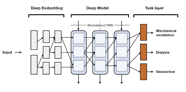
SeqSNR is a time series adaptation of the SNR architecture and is a combination of a deep embedding layer followed by stacked recurrent neural network (RNN) layers. Modularisation is achieved by splitting both the embedding layer and the RNN stack into multiple modules connected by routing variables that are learned during the training phase. The routing connections are always created between blocks in one layer and the next. This approach minimizes negative transfer by ensuring that data of low relevance to a particular task layer is filtered out. In essence, this means that each task utilizes a different path through the model.

A high-level overview of the SeqSNR architecture.

Findings
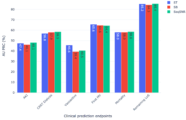
SeqSNR shows a modest improvement in discriminative performance overall relative to single-task and naïve multitasking. However, it's performance improvement is more significant in scenarios with few training labels.

Because the prevalence of different outcomes varied widely in the dataset (e.g. ~38% of patients had MV, but CRRT dialysis is present for only ~3%), many accuracy metrics are not suitable. Instead, we report the area under the precision recall curve (AU PRC), which is more reliable given imbalanced data. Moreover, we performed the Wilcoxon Signed Rank Tests to draw statistically significant conclusions for pairwise comparisons of ST learning, shared-bottom (SB) multi-task learning (i.e., naïve multi-task learning), and SeqSNR across bootstrapped samples from the held-out test set. The performance differences between the three architectures were modest, but SeqSNR outperformed both ST and SB in four out of six tasks (p-values are reported in the paper).

Comparison of single task (ST), shared bottom (SB) and SeqSNR performance on the MIMIC-III dataset.

Label Efficiency
We hypothesized that multi-task learning could assist in low-data scenarios by using easy-to-label auxiliary tasks to boost the performance of the main tasks. We formulated prediction tasks with only a portion of the training labels available for the primary prediction task, but kept the entire dataset for the “helper tasks”. The latter are chosen because they are reliably encoded in the EHR and are straightforward to timestamp. An example of such a helper task is length of stay, since the start and end of admissions are accurately timestamped in MIMIC-III. On the other hand, the start and end of mechanical ventilation events are not reliably timestamped. So, we defined a set of rules based on expert-defined heuristics to determine the ventilation times using multiple sources of mechanical ventilator–related settings along with physiological measurements in the EHR dataset that are indicative of MV.

The development of these rules for a new clinical endpoint was time-consuming and involved manual review of the dataset by experts. The difficulty in exhaustively labeling the dataset led us to test the model performance with only 1–10% of the data labeled, which resulted in a decline in model performance. The “helper tasks” are useful in this scenario since they are 100% labeled and can be used with the primary tasks (1–10% labeled) to jointly train the multi-task model for improved overall performance.

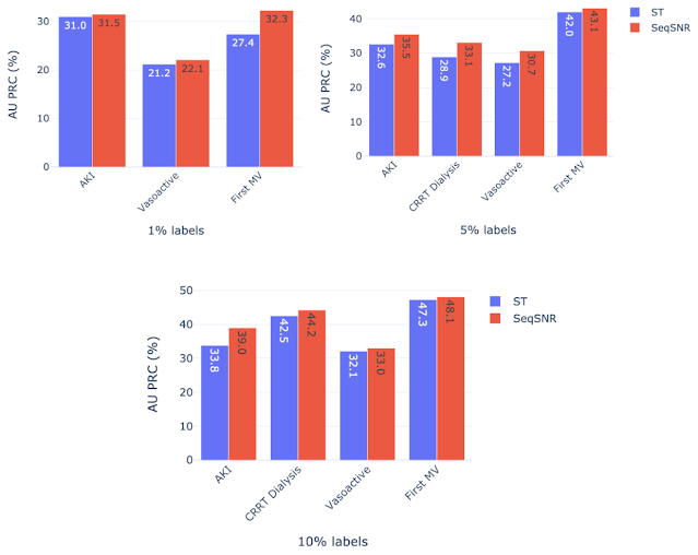
We chose AKI, mechanical ventilation, CRRT Dialysis, and vasoactive medications as primary endpoints using 1%, 5%, and 10% of the training labels, along with 100% of labels for the helper tasks — labs and vitals, mortality, and LoS. Performance of both ST and SeqSNR decreased as the percentage of labels for the primary endpoint was reduced, but SeqSNR outperformed ST across all tasks and all training data reduction percentages, with a statistically significant boost in performance for all cases.

Label efficiency results showing the discriminative performance when the training dataset for the primary endpoint is reduced to 1%, 5% and 10% while the helper tasks have access to all training labels.

This is a useful finding, given the difficulties of annotating endpoint labels in EHR datasets, which frequently necessitates human evaluation by doctors. The ability to use numerous endpoints, some of which may be easier to label (like duration of stay or mortality), could lessen the need for manual curation on more difficult endpoints that are annotated differently (like mechanical ventilation).

Subgroup Performance
While the version of the MIMIC-III dataset used contained labels for gender and age, it did not contain information on race and the information on ethnicity was limited. We computed the performance of all selected models across age and gender subgroups. We observed that in the scenarios with few instances in the dataset, the MTL models (both SB models and SeqSNR) often outperform ST. Even though there are exceptions, on average all models seem to be relatively balanced across age and gender subgroups. We invite the reader to refer to the supplemental section of our paper for a detailed performance breakdown.

Next Steps
This work is a proof of concept for SeqSNR on a set of canonical EHR prediction tasks. The code for this architecture is publicly available here. And will hopefully stimulate further research in EHR multi-tasking and other deep learning architectures inspired by clinical reasoning.

In future, it will be important to evaluate the performance of SeqSNR on different combinations of tasks, different time horizons and different datasets. One other area of potential growth in this project is to expand subgroup analysis by including datasets with additional population information, race, ethnicity, etc. Another area we are exploring is expanding subgroup analysis by including datasets with additional population information, such as race, ethnicity, etc. We also emphasize that these are prototype models designed to showcase methodologies, and more rigorous evaluation would be needed to bring these tools into deployment.

Acknowledgements
This work involved collaborative efforts from a multidisciplinary team of researchers, software engineers, clinicians, and cross-functional contributors. We thank our co-authors: Eric Loreaux, Anne Mottram, Ivan Protsyuk, Natalie Harris, Sebastien Baur, Yuan Xue, Jessica Schrouff, Ali Connell, Alan Karthikesalingam, Martin Seneviratne from Google, Nenad Tomasev from Deepmind, and Hugh Montgomery from University College London. We also thank Zhe Zhao from Google Research and Kathryn Rough, Cian Hughes, Megumi Morigami and Doris Wong from Google Health for their input and review, and the MIMIC team for curating this open access dataset for the research community.

Source: Google AI Blog