Tag Archives: Physics

Introducing TensorNetwork, an Open Source Library for Efficient Tensor Calculations


Many of the world's toughest scientific challenges, like developing high-temperature superconductors and understanding the true nature of space and time, involve dealing with the complexity of quantum systems. What makes these challenges difficult is that the number of quantum states in these systems is exponentially large, making brute-force computation infeasible. To deal with this, data structures called tensor networks are used. Tensor networks let one focus on the quantum states that are most relevant for real-world problems—the states of low energy, say—while ignoring other states that aren't relevant. Tensor networks are also increasingly finding applications in machine learning (ML). However, there remain difficulties that prohibit them from widespread use in the ML community: 1) a production-level tensor network library for accelerated hardware has not been available to run tensor network algorithms at scale, and 2) most of the tensor network literature is geared toward physics applications and creates the false impression that expertise in quantum mechanics is required to understand the algorithms.

In order to address these issues, we are releasing TensorNetwork, a brand new open source library to improve the efficiency of tensor calculations, developed in collaboration with the Perimeter Institute for Theoretical Physics and X. TensorNetwork uses TensorFlow as a backend and is optimized for GPU processing, which can enable speedups of up to 100x when compared to work on a CPU. We introduce TensorNetwork in a series of papers, the first of which presents the new library and its API, and provides an overview of tensor networks for a non-physics audience. In our second paper we focus on a particular use case in physics, demonstrating the speedup that one gets using GPUs.

How are Tensor Networks Useful?
Tensors are multidimensional arrays, categorized in a hierarchy according to their order: e.g., an ordinary number is a tensor of order zero (also known as a scalar), a vector is an order-one tensor, a matrix is an order-two tensor, and so on. While low-order tensors can easily be represented by an explicit array of numbers or with a mathematical symbol such as Tijnklm (where the number of indices represents the order of the tensor), that notation becomes very cumbersome once we start talking about high-order tensors. At that point it’s useful to start using diagrammatic notation, where one simply draws a circle (or some other shape) with a number of lines, or legs, coming out of it—the number of legs being the same as the order of the tensor. In this notation, a scalar is just a circle, a vector has a single leg, a matrix has two legs, etc. Each leg of the tensor also has a dimension, which is the size of that leg. For example, a vector representing an object’s velocity through space would be a three-dimensional, order-one tensor.


Diagrammatic notation for tensors.
The benefit of representing tensors in this way is to succinctly encode mathematical operations, e.g., multiplying a matrix by a vector to produce another vector, or multiplying two vectors to make a scalar. These are all examples of a more general concept called tensor contraction.

Diagrammatic notation for tensor contraction. Vector and matrix multiplication, as well as the matrix trace (i.e., the sum of the diagonal elements of a matrix), are all examples.
These are also simple examples of tensor networks, which are graphical ways of encoding the pattern of tensor contractions of several constituent tensors to form a new one. Each constituent tensor has an order determined by its own number of legs. Legs that are connected, forming an edge in the diagram, represent contraction, while the number of remaining dangling legs determines the order of the resultant tensor.
Left: The trace of the product of four matrices, tr(ABCD), which is a scalar. You can see that it has no dangling legs. Right: Three order-three tensors being contracted with three legs dangling, resulting in a new order-three tensor.
While these examples are very simple, the tensor networks of interest often represent hundreds of tensors contracted in a variety of ways. Describing such a thing would be very obscure using traditional notation, which is why the diagrammatic notation was invented by Roger Penrose in 1971.

Tensor Networks in Practice
Consider a collection of black-and-white images, each of which can be thought of as a list of N pixel values. A single pixel of a single image can be one-hot-encoded into a two-dimensional vector, and by combining these pixel encodings together we can make a 2N-dimensional one-hot encoding of the entire image. We can reshape that high-dimensional vector into an order-N tensor, and then add up all of the tensors in our collection of images to get a total tensor Ti1,i2,...,iN encapsulating the collection.

This sounds like a very wasteful thing to do: encoding images with about 50 pixels in this way would already take petabytes of memory. That’s where tensor networks come in. Rather than storing or manipulating the tensor T directly, we instead represent T as the contraction of many smaller constituent tensors in the shape of a tensor network. That turns out to be much more efficient. For instance, the popular matrix product state (MPS) network would write T in terms of N much smaller tensors, so that the total number of parameters is only linear in N, rather than exponential.
The high-order tensor T is represented in terms of many low-order tensors in a matrix product state tensor network.
It’s not obvious that large tensor networks can be efficiently created or manipulated while consistently avoiding the need for a huge amount of memory. But it turns out that this is possible in many cases, which is why tensor networks have been used extensively in quantum physics and, now, in machine learning. Stoudenmire and Schwab used the encoding just described to make an image classification model, demonstrating a new use for tensor networks. The TensorNetwork library is designed to facilitate exactly that kind of work, and our first paper describes how the library functions for general tensor network manipulations.

Performance in Physics Use-Cases
TensorNetwork is a general-purpose library for tensor network algorithms, and so it should prove useful for physicists as well. Approximating quantum states is a typical use-case for tensor networks in physics, and is well-suited to illustrate the capabilities of the TensorNetwork library. In our second paper, we describe a tree tensor network (TTN) algorithm for approximating the ground state of either a periodic quantum spin chain (1D) or a lattice model on a thin torus (2D), and implement the algorithm using TensorNetwork. We compare the use of CPUs with GPUs and observe significant computational speed-ups, up to a factor of 100, when using a GPU and the TensorNetwork library.
Computational time as a function of the bond dimension, χ. The bond dimension determines the size of the constituent tensors of the tensor network. A larger bond dimension means the tensor network is more powerful, but requires more computational resources to manipulate.
Conclusion and Future Work
These are the first in a series of planned papers to illustrate the power of TensorNetwork in real-world applications. In our next paper we will use TensorNetwork to classify images in the MNIST and Fashion-MNIST datasets. Future plans include time series analysis on the ML side, and quantum circuit simulation on the physics side. With the open source community, we are also always adding new features to TensorNetwork itself. We hope that TensorNetwork will become a valuable tool for physicists and machine learning practitioners.

Acknowledgements
The TensorNetwork library was developed by Chase Roberts, Adam Zalcman, and Bruce Fontaine of Google AI; Ashley Milsted, Martin Ganahl, and Guifre Vidal of the Perimeter Institute; and Jack Hidary and Stefan Leichenauer of X. We’d also like to thank Stavros Efthymiou at X for valuable contributions.

Source: Google AI Blog


Unifying Physics and Deep Learning with TossingBot


Though considerable progress has been made in enabling robots to grasp objects efficiently, visually self adapt or even learn from real-world experiences, robotic operations still require careful consideration in how they pick up, handle, and place various objects -- especially in unstructured settings. Consider for example, this picking robot which took 1st place in the stowing task of the Amazon Robotics Challenge:
It's an impressive system, built with many design features that kinematically prevent it from dropping objects due to unforeseen dynamics: from its steady and deliberate movements, to its gripper fingers that mechanically constrain the momentum of the object so that it doesn't slip.

This robot, like many others, is designed to tolerate the dynamics of the unstructured world. But instead of just tolerating dynamics, can robots learn to use them advantageously, developing an "intuition" of physics that would allow them to complete tasks more efficiently? Perhaps in doing so, robots can improve their capabilities and acquire complex athletic skills like tossing, sliding, spinning, swinging, or catching, potentially leading to many useful applications, such as more efficient debris clearing robots in disaster response scenarios -- where time is of the essence.

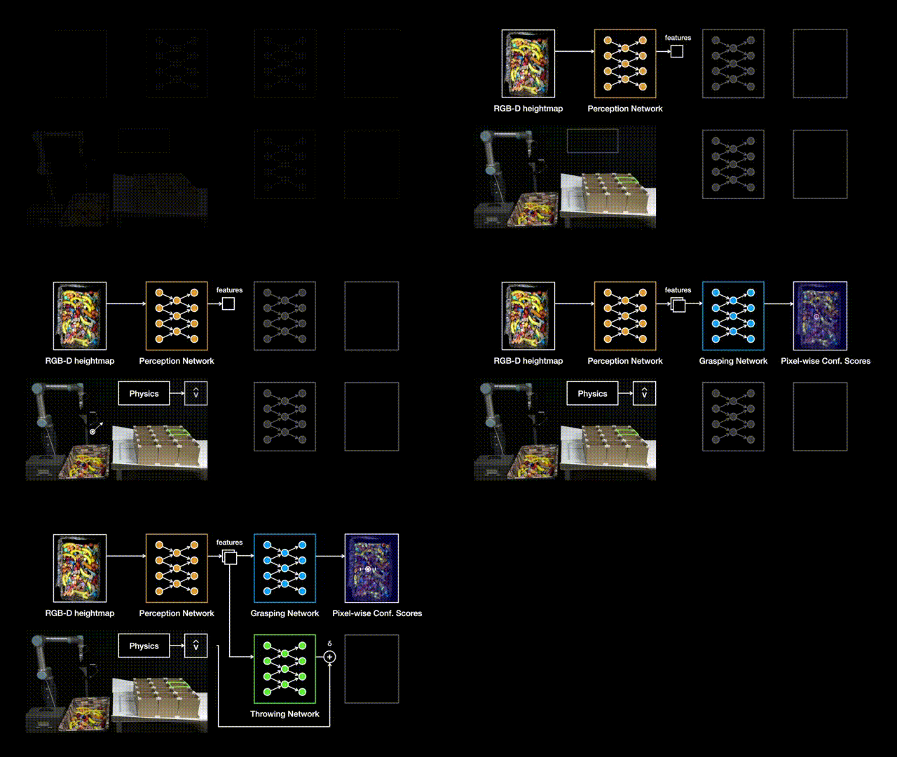
To explore this concept, we worked with researchers at Princeton, Columbia, and MIT to develop TossingBot: a picking robot for our real, random world that learns to grasp and throw objects into selected boxes outside its natural range. We find that by learning to throw, TossingBot is capable of achieving picking speeds that are twice as fast as previous systems, with twice the effective placing range. TossingBot jointly learns grasping and throwing policies using an end-to-end neural network that maps from visual observations (RGB-D images) to control parameters for motion primitives. Using overhead cameras to track where objects land, TossingBot improves itself over time through self-supervision. More technical details are available in an early preprint on arXiv.
The Challenges
Throwing is a particularly difficult task as it depends on many factors: from how the object is picked up (i.e., "pre-throw conditions"), to the object's physical properties like mass, friction, aerodynamics, etc. For example, if you grasp a screwdriver by the handle near the center of mass and throw it, it would land much closer than if you had grasped it from the metal tip, which would swing forward and land much farther away. Regardless of how you grasped it though, tossing a screwdriver is incredibly different from tossing a ping pong ball, which would land closer due to air resistance. Manually designing a solution that explicitly handles these factors for every random object is nearly impossible.
Throwing depends on many factors: from how you picked it up, to object properties and dynamics.
Through deep learning, however, our robots can learn from experience rather than rely on manual case-by-case engineering. Previously we've shown that our robots can learn to push and grasp a large variety of objects, but accurately throwing objects requires a larger understanding of projectile physics. Acquiring this knowledge from scratch with only trial-and-error is not only time consuming and expensive, but also generally doesn't work outside of very specific, and carefully set up training scenarios.

Unifying Physics and Deep Learning
A fundamental component of TossingBot is that it learns to throw by integrating simple physics and deep learning, which enables it to train quickly and generalize to new scenarios. Physics provides prior models of how the world works, and we can leverage these models to develop initial controllers for our robots. In the case of throwing, for example, we can use projectile ballistics to provide an estimate for the throwing velocity that is needed to get an object to land at a target location. We can then use neural networks to predict adjustments on top of that estimate from physics, in order to compensate for unknown dynamics as well as the noise and variability of the real world. We call this hybrid formulation Residual Physics, and it enables TossingBot to achieve throwing accuracies of 85%.
At the start of training with randomly initialized weights, TossingBot repeatedly attempts bad grasps. Over time, however, TossingBot learns better ways to grasp objects and simultaneously improves its ability to throw. Occasionally the robot randomly explores what happens if it throws an object at a velocity that it hasn't tried before. When the bin is emptied, TossingBot lifts the boxes to allow objects to slide back into the bin. This way, human intervention is kept at a minimum during training. By 10,000 grasp and throw attempts (or 14 hours of training time), it is capable of achieving throwing accuracies of 85%, with a grasping reliability of 87% in clutter.
TossingBot starts out performing poorly (left), but progressively learns to grasp and toss overnight (right).
Generalizing to New Scenarios
By integrating physics and deep learning, TossingBot is capable of rapidly adapting to never-before-seen throwing locations and objects. For example, after training on objects with simple shapes like wooden blocks, balls, and markers, it can perform reasonably well on new objects such as fake fruit, decorative items, and office objects. On new objects, TossingBot starts out with lower performance, but quickly adapts within a few hundred training steps (i.e., an hour or two) to achieve similar performance as with training objects. We've found that combining physics and deep learning with Residual Physics yields better performance than baseline alternatives (e.g. deep learning without physics). We even tried this task ourselves, and we were pleasantly surprised to learn that TossingBot is more accurate than any of us engineers! Though take that with a grain of salt, as we've yet to test TossingBot against anyone with any actual athletic talent.
TossingBot can generalize to new objects, and is more accurate at throwing than the average Googler.
We also test our policies on their ability to generalize to new target locations previously unseen in training. To this end, we train on a set of boxes, then later test on a different set of boxes with entirely different landing areas. In this setting, we find that Residual Physics for throwing helps significantly, since the initial estimates of throwing velocities from projectile ballistics easily generalize to new target locations, while the residuals help make adjustments on top of those estimates to compensate for varying object properties in the real world. This is in contrast to the baseline alternative of using deep learning without physics, which can only handle target locations seen during training.
TossingBot uses Residual Physics to throw objects to unforeseen locations.
Emerging Semantics from Interaction
To explore what TossingBot learns, we place several objects in the bin, capture images, and feed them into TossingBot's trained neural network to extract intermediate pixel-wise deep features. By clustering these features based on similarity and visualizing nearest neighbors as a heatmap (hotter regions indicate more similarity in feature space), we can localize all ping pong balls in the scene. Even though the orange block shares a similar color with the ping pong balls, its features are different enough for TossingBot to make a distinction. Likewise, we can also use the extracted features to localize all marker pens, which share similar shape and mass, but do not share color. These observations suggest that TossingBot likely learns to rely more on geometric cues (e.g. shape) to learn grasping and throwing. It is also possible that the learned features reflect second-order attributes such as physical properties, which can influence how the objects should be thrown.
TossingBot learns deep features that distinguish object categories without explicit supervision.
These emerging features were learned implicitly from scratch without any explicit supervision beyond task-level grasping and throwing. Yet, they seem to be sufficient for enabling the system to distinguish between object categories (i.e., ping pong balls and marker pens). As such, this experiment speaks out to a broader concept related to machine vision: how should robots learn the semantics of the visual world? From the perspective of classic computer vision, semantics are often pre-defined using human-fabricated image datasets and manually constructed class categories. However, our experiment suggests that it is possible to implicitly learn such object-level semantics from physical interactions alone, as long as they matter for the task at hand. The more complex these interactions, the higher the resolution of the semantics. Towards more generally intelligent robots -- perhaps it is sufficient for them to develop their own notion of semantics through interaction, without requiring any human intervention.

Limitations and Future Work
Although TossingBot's results are promising, it does have its limitations. For example, it assumes that objects are robust enough to withstand landing collisions after being thrown -- further work is required to learn throws that account for fragile objects, or possibly train other robots to catch objects in ways that cushion the landing. Furthermore, TossingBot infers control parameters only from visual data -- exploring additional senses (e.g. force-torque or tactile) may enable the system to better react to new objects.

The combination of physics and deep learning that made TossingBot possible naturally leads to an interesting question: what else could benefit from Residual Physics? Investigating how the idea generalizes to other types of tasks and interactions is a promising direction for future research.

You can learn more about this work in the summary video below.
Acknowledgements
This research was done by Andy Zeng, Shuran Song (faculty at Columbia University), Johnny Lee, Alberto Rodriguez (faculty at MIT), and Thomas Funkhouser (faculty at Princeton University), with special thanks to Ryan Hickman for valuable managerial support, Ivan Krasin and Stefan Welker for fruitful technical discussions, Brandon Hurd and Julian Salazar and Sean Snyder for hardware support, Chad Richards and Jason Freidenfelds for helpful feedback on writing, Erwin Coumans for advice on PyBullet, Laura Graesser for video narration, and Regina Hickman for photography. An early preprint is available on arXiv.

Source: Google AI Blog


The Question of Quantum Supremacy


Quantum computing integrates the two largest technological revolutions of the last half century, information technology and quantum mechanics. If we compute using the rules of quantum mechanics, instead of binary logic, some intractable computational tasks become feasible. An important goal in the pursuit of a universal quantum computer is the determination of the smallest computational task that is prohibitively hard for today’s classical computers. This crossover point is known as the “quantum supremacy” frontier, and is a critical step on the path to more powerful and useful computations.

In “Characterizing quantum supremacy in near-term devices” published in Nature Physics (arXiv here), we present the theoretical foundation for a practical demonstration of quantum supremacy in near-term devices. It proposes the task of sampling bit-strings from the output of random quantum circuits, which can be thought of as the “hello world” program for quantum computers. The upshot of the argument is that the output of random chaotic systems (think butterfly effect) become very quickly harder to predict the longer they run. If one makes a random, chaotic qubit system and examines how long a classical system would take to emulate it, one gets a good measure of when a quantum computer could outperform a classical one. Arguably, this is the strongest theoretical proposal to prove an exponential separation between the computational power of classical and quantum computers.

Determining where exactly the quantum supremacy frontier lies for sampling random quantum circuits has rapidly become an exciting area of research. On one hand, improvements in classical algorithms to simulate quantum circuits aim to increase the size of the quantum circuits required to establish quantum supremacy. This forces an experimental quantum device with a sufficiently large number of qubits and low enough error rates to implement circuits of sufficient depth (i.e the number of layers of gates in the circuit) to achieve supremacy. On the other hand, we now understand better how the particular choice of the quantum gates used to build random quantum circuits affects the simulation cost, leading to improved benchmarks for near-term quantum supremacy (available for download here), which are in some cases quadratically more expensive to simulate classically than the original proposal.

Sampling from random quantum circuits is an excellent calibration benchmark for quantum computers, which we call cross-entropy benchmarking. A successful quantum supremacy experiment with random circuits would demonstrate the basic building blocks for a large-scale fault-tolerant quantum computer. Furthermore, quantum physics has not yet been tested for highly complex quantum states such as this.
Space-time volume of a quantum circuit computation. The computational cost for quantum simulation increases with the volume of the quantum circuit, and in general grows exponentially with the number of qubits and the circuit depth. For asymmetric grids of qubits, the computational space-time volume grows slower with depth than for symmetric grids, and can result in circuits exponentially easier to simulate.
In “A blueprint for demonstrating quantum supremacy with superconducting qubits” (arXiv here), we illustrate a blueprint towards quantum supremacy and experimentally demonstrate a proof-of-principle version for the first time. In the paper, we discuss two key ingredients for quantum supremacy: exponential complexity and accurate computations. We start by running algorithms on subsections of the device ranging from 5 to 9 qubits. We find that the classical simulation cost grows exponentially with the number of qubits. These results are intended to provide a clear example of the exponential power of these devices. Next, we use cross-entropy benchmarking to compare our results against that of an ordinary computer and show that our computations are highly accurate. In fact, the error rate is low enough to achieve quantum supremacy with a larger quantum processor.

Beyond achieving quantum supremacy, a quantum platform should offer clear applications. In our paper, we apply our algorithms towards computational problems in quantum statistical-mechanics using complex multi-qubit gates (as opposed to the two-qubit gates designed for a digital quantum processor with surface code error correction). We show that our devices can be used to study fundamental properties of materials, e.g. microscopic differences between metals and insulators. By extending these results to next-generation devices with ~50 qubits, we hope to answer scientific questions that are beyond the capabilities of any other computing platform.
Photograph of two gmon superconducting qubits and their tunable coupler developed by Charles Neill and Pedram Roushan.
These two publications introduce a realistic proposal for near-term quantum supremacy, and demonstrate a proof-of-principle version for the first time. We will continue to decrease the error rates and increase the number of qubits in quantum processors to reach the quantum supremacy frontier, and to develop quantum algorithms for useful near-term applications.

Source: Google AI Blog


Reformulating Chemistry for More Efficient Quantum Computation


The first known classical “computer” was the Antikythera mechanism, an analog machine used to simulate the classical mechanics governing dynamics of celestial bodies on an astronomical scale. Similarly, a major ambition of quantum computers is to simulate the quantum mechanics governing dynamics of particles on the atomic scale. These simulations are often classically intractable due to the complex quantum mechanics at play. Of particular interest is the simulation of electrons forming chemical bonds, which give rise to the properties of essentially all molecules, materials and chemical reactions.
Left: The first known computing device, the Antikythera mechanism: a classical machine used to simulate classical mechanics. Right: Google’s 22 Xmon qubit “foxtail” chip arranged in a bilinear array on a wafer, the predecessor to Google’s new Bristlecone quantum processor with 72 qubits, a quantum machine we intend to use to simulate quantum mechanics, among other applications.
Since the launch of the Quantum AI team in 2013, we have been developing practical algorithms for quantum processors. In 2015, we conducted the first quantum chemistry experiment on a superconducting quantum computing device, published in Physical Review X. More recently, our quantum simulation effort experimentally simulated exotic phases of matter and released the first software package for quantum computing chemistry, OpenFermion. Earlier this month, our hardware team announced the new Bristlecone quantum processor with 72 qubits.

Today, we highlight two recent publications with theoretical advances that significantly reduce the cost of these quantum computations. Our results were presented at the Quantum Information Processing and IBM ThinkQ conferences.

The first of these works, “Low-Depth Quantum Simulation of Materials,” published this week in Physical Review X, was a collaboration between researchers at Google, the group of Professor Garnet Chan at Caltech and the QuArC group at Microsoft. Our fundamental advance was to realize that by changing how molecules are represented on quantum computers, we can greatly simplify the quantum circuits required to solve the problem. Specifically, we specially design basis sets so that the equations describing the system energies (i.e. the Hamiltonian) become more straightforward to express for quantum computation.

To do this, we focused on using basis sets related to functions (plane waves) used in classical electronic structure calculations to provide a periodic representation of the physical system. This enables one to go beyond the quantum simulation of single-molecules and instead use quantum computers to model realistic materials. For instance, instead of simulating a single lithium hydride molecule floating in free space, with our approach one can quantum simulate a crystal of lithium hydride, which is how the material appears in nature. With larger quantum computers one could study other important materials problems such as the degradation of battery cathodes, chemical reactions involving heterogeneous catalysts, or the unusual electrical properties of graphene and superconductors.

In “Quantum Simulation of Electronic Structure with Linear Depth and Connectivity,” published last week in Physical Review Letters with the same collaborators and a Google intern from the Aspuru-Guzik group at Harvard, we leverage the structure introduced in the work above to design algorithms for near-term quantum computers with qubits laid out in a linear array. Whereas past methods required such quantum computers to run for time scaling as the fifth power of the number of simulated electrons for each dynamic step, our improved algorithm runs for time scaling linearly with respect to the number of electrons. This reduction in computational cost makes it viable to perform quantum chemistry simulations on near-term devices with fewer gates in each quantum circuit, possibly avoiding the need for full error-correction.

Even with these improvements, it is no small task to deploy such new technology to outperform classical quantum chemistry algorithms and methods which have been refined in parallel with the development of classical computers for more than eighty years. However, at the current rate of advances in quantum algorithms and hardware, quantum technologies may provide chemists with an invaluable new tool. We look forward to sharing our research results as they develop.

Source: Google AI Blog


Announcing OpenFermion: The Open Source Chemistry Package for Quantum Computers

Crossposted on the Google Research Blog

“The underlying physical laws necessary for the mathematical theory of a large part of physics and the whole of chemistry are thus completely known, and the difficulty is only that the exact application of these laws leads to equations much too complicated to be soluble.”
-Paul Dirac, Quantum Mechanics of Many-Electron Systems (1929)

In this passage, physicist Paul Dirac laments that while quantum mechanics accurately models all of chemistry, exactly simulating the associated equations appears intractably complicated. Not until 1982 would Richard Feynman suggest that instead of surrendering to the complexity of quantum mechanics, we might harness it as a computational resource. Hence, the original motivation for quantum computing: by operating a computer according to the laws of quantum mechanics, one could efficiently unravel exact simulations of nature. Such simulations could lead to breakthroughs in areas such as photovoltaics, batteries, new materials, pharmaceuticals and superconductivity. And while we do not yet have a quantum computer large enough to solve classically intractable problems in these areas, rapid progress is being made. Last year, Google published this paper detailing the first quantum computation of a molecule using a superconducting qubit quantum computer. Building on that work, the quantum computing group at IBM scaled the experiment to larger molecules, which made the cover of Nature last month.

Today, we announce the release of OpenFermion, the first open source platform for translating problems in chemistry and materials science into quantum circuits that can be executed on existing platforms. OpenFermion is a library for simulating the systems of interacting electrons (fermions) which give rise to the properties of matter. Prior to OpenFermion, quantum algorithm developers would need to learn a significant amount of chemistry and write a large amount of code hacking apart other codes to put together even the most basic quantum simulations. While the project began at Google, collaborators at ETH Zurich, Lawrence Berkeley National Labs, University of Michigan, Harvard University, Oxford University, Dartmouth College, Rigetti Computing and NASA all contributed to alpha releases. You can learn more details about this release in our paper, OpenFermion: The Electronic Structure Package for Quantum Computers.

One way to think of OpenFermion is as a tool for generating and compiling physics equations which describe chemical and material systems into representations which can be interpreted by a quantum computer1. The most effective quantum algorithms for these problems build upon and extend the power of classical quantum chemistry packages used and developed by research chemists across government, industry and academia. Accordingly, we are also releasing OpenFermion-Psi4 and OpenFermion-PySCF which are plugins for using OpenFermion in conjunction with the classical electronic structure packages Psi4 and PySCF.

The core OpenFermion library is designed in a quantum programming framework agnostic way to ensure compatibility with various platforms being developed by the community. This allows OpenFermion to support external packages which compile quantum assembly language specifications for diverse hardware platforms. We hope this decision will help establish OpenFermion as a community standard for putting quantum chemistry on quantum computers. To see how OpenFermion is used with diverse quantum programming frameworks, take a look at OpenFermion-ProjectQ and Forest-OpenFermion - plugins which link OpenFermion to the externally developed circuit simulation and compilation platforms known as ProjectQ and Forest.

The following workflow describes how a quantum chemist might use OpenFermion in order to simulate the energy surface of a molecule (for instance, by preparing the sort of quantum computation we described in our past blog post):
  1. The researcher initializes an OpenFermion calculation with specification of:
    • An input file specifying the coordinates of the nuclei in the molecule.
    • The basis set (e.g. cc-pVTZ) that should be used to discretize the molecule.
    • The charge and spin multiplicity (if known) of the system.
  1. The researcher uses the OpenFermion-Psi4 plugin or the OpenFermion-PySCF plugin to perform scalable classical computations which are used to optimally stage the quantum computation. For instance, one might perform a classical Hartree-Fock calculation to choose a good initial state for the quantum simulation.
  2. The researcher then specifies which electrons are most interesting to study on a quantum computer (known as an active space) and asks OpenFermion to map the equations for those electrons to a representation suitable for quantum bits, using one of the available procedures in OpenFermion, e.g. the Bravyi-Kitaev transformation.
  3. The researcher selects a quantum algorithm to solve for the properties of interest and uses a quantum compilation framework such as OpenFermion-ProjectQ to output the quantum circuit in assembly language which can be run on a quantum computer. If the researcher has access to a quantum computer, they then execute the experiment.
A few examples of what one might do with OpenFermion are demonstrated in ipython notebooks here, here and here. While quantum simulation is widely recognized as one of the most important applications of quantum computing in the near term, very few quantum computer scientists know quantum chemistry and even fewer chemists know quantum computing. Our hope is that OpenFermion will help to close the gap between these communities and bring the power of quantum computing to chemists and material scientists. If you’re interested, please checkout our GitHub repository - pull requests welcome! By Ryan Babbush and Jarrod McClean, Quantum Software Engineers, Quantum AI Team

1 If we may be allowed one sentence for the experts: the primary function of OpenFermion is to encode the electronic structure problem in second quantization defined by various basis sets and active spaces and then to transform those operators into spin Hamiltonians using various isomorphisms between qubit and fermion algebras.

Announcing OpenFermion: The Open Source Chemistry Package for Quantum Computers


“The underlying physical laws necessary for the mathematical theory of a large part of physics and the whole of chemistry are thus completely known, and the difficulty is only that the exact application of these laws leads to equations much too complicated to be soluble.”
-Paul Dirac, Quantum Mechanics of Many-Electron Systems (1929)

In this passage, physicist Paul Dirac laments that while quantum mechanics accurately models all of chemistry, exactly simulating the associated equations appears intractably complicated. Not until 1982 would Richard Feynman suggest that instead of surrendering to the complexity of quantum mechanics, we might harness it as a computational resource. Hence, the original motivation for quantum computing: by operating a computer according to the laws of quantum mechanics, one could efficiently unravel exact simulations of nature. Such simulations could lead to breakthroughs in areas such as photovoltaics, batteries, new materials, pharmaceuticals and superconductivity. And while we do not yet have a quantum computer large enough to solve classically intractable problems in these areas, rapid progress is being made. Last year, Google published this paper detailing the first quantum computation of a molecule using a superconducting qubit quantum computer. Building on that work, the quantum computing group at IBM scaled the experiment to larger molecules, which made the cover of Nature last month.

Today, we announce the release of OpenFermion, the first open source platform for translating problems in chemistry and materials science into quantum circuits that can be executed on existing platforms. OpenFermion is a library for simulating the systems of interacting electrons (fermions) which give rise to the properties of matter. Prior to OpenFermion, quantum algorithm developers would need to learn a significant amount of chemistry and write a large amount of code hacking apart other codes to put together even the most basic quantum simulations. While the project began at Google, collaborators at ETH Zurich, Lawrence Berkeley National Labs, University of Michigan, Harvard University, Oxford University, Dartmouth University, Rigetti Computing and NASA all contributed to alpha releases. You can learn more details about this release in our paper, OpenFermion: The Electronic Structure Package for Quantum Computers.

One way to think of OpenFermion is as a tool for generating and compiling physics equations which describe chemical and material systems into representations which can be interpreted by a quantum computer1. The most effective quantum algorithms for these problems build upon and extend the power of classical quantum chemistry packages used and developed by research chemists across government, industry and academia. Accordingly, we are also releasing OpenFermion-Psi4 and OpenFermion-PySCF which are plugins for using OpenFermion in conjunction with the classical electronic structure packages Psi4 and PySCF.

The core OpenFermion library is designed in a quantum programming framework agnostic way to ensure compatibility with various platforms being developed by the community. This allows OpenFermion to support external packages which compile quantum assembly language specifications for diverse hardware platforms. We hope this decision will help establish OpenFermion as a community standard for putting quantum chemistry on quantum computers. To see how OpenFermion is used with diverse quantum programming frameworks, take a look at OpenFermion-ProjectQ and Forest-OpenFermion - plugins which link OpenFermion to the externally developed circuit simulation and compilation platforms known as ProjectQ and Forest.

The following workflow describes how a quantum chemist might use OpenFermion in order to simulate the energy surface of a molecule (for instance, by preparing the sort of quantum computation we described in our past blog post):
  1. The researcher initializes an OpenFermion calculation with specification of:
    • An input file specifying the coordinates of the nuclei in the molecule.
    • The basis set (e.g. cc-pVTZ) that should be used to discretize the molecule.
    • The charge and spin multiplicity (if known) of the system.
  1. The researcher uses the OpenFermion-Psi4 plugin or the OpenFermion-PySCF plugin to perform scalable classical computations which are used to optimally stage the quantum computation. For instance, one might perform a classical Hartree-Fock calculation to choose a good initial state for the quantum simulation.
  2. The researcher then specifies which electrons are most interesting to study on a quantum computer (known as an active space) and asks OpenFermion to map the equations for those electrons to a representation suitable for quantum bits, using one of the available procedures in OpenFermion, e.g. the Bravyi-Kitaev transformation.
  3. The researcher selects a quantum algorithm to solve for the properties of interest and uses a quantum compilation framework such as OpenFermion-ProjectQ to output the quantum circuit in assembly language which can be run on a quantum computer. If the researcher has access to a quantum computer, they then execute the experiment.
A few examples of what one might do with OpenFermion are demonstrated in ipython notebooks here, here and here. While quantum simulation is widely recognized as one of the most important applications of quantum computing in the near term, very few quantum computer scientists know quantum chemistry and even fewer chemists know quantum computing. Our hope is that OpenFermion will help to close the gap between these communities and bring the power of quantum computing to chemists and material scientists. If you’re interested, please checkout our GitHub repository - pull requests welcome!


1 If we may be allowed one sentence for the experts: the primary function of OpenFermion is to encode the electronic structure problem in second quantization defined by various basis sets and active spaces and then to transform those operators into spin Hamiltonians using various isomorphisms between qubit and fermion algebras.

So there I was, firing a megawatt plasma collider at work…


Wait, what? Why is Google interested in plasma physics?

Google is always interested in solving complex engineering problems, and few are more complex than fusion. Physicists have been trying since the 1950s to control the fusion of hydrogen atoms into helium, which is the same process that powers the Sun. The key to harnessing this power is to confine hydrogen plasmas for long enough to get more energy out from fusion reactions than was put in. This point is called “breakeven.” If it works, it would represent a technological breakthrough, and could provide an abundant source of zero-carbon energy.

There are currently several large academic and government research efforts in fusion. Just to rattle off a few, in plasma fusion there are tokamak machines like ITER and stellarator machines like Wendelstein 7-X. The stellarator design actually goes back to 1951, so physicists have been working on this for a while. Oh yeah, and if you like giant lasers, there’s the National Ignition Facility which users lasers to generate X-rays to generate fusion reactions. So far, none of these has gotten to the economic breakeven point.

All of these efforts involve complex experiments with many variables, providing an opportunity for Google to help, with our strength in computing and machine learning. Today, we’re publishing “Achievement of Sustained Net Plasma Heating in a Fusion Experiment with the Optometrist Algorithm” in Scientific Reports. This paper describes the first results of Google’s collaboration with the physicists and engineers at Tri Alpha Energy, taking a step towards the breakeven goal.

Did you really just say that you got to fire a plasma collider?

Yeah. Tri Alpha Energy has a unique scheme for plasma confinement called a field-reversed configuration that’s predicted to get more stable as the energy goes up, in contrast to other methods where plasmas get harder to control as you heat them. Tri Alpha built a giant ionized plasma machine, C-2U, that fills an entire warehouse in an otherwise unassuming office park. The plasma that this machine generates and confines exhibits all kinds of highly nonlinear behavior. The machine itself pushes the envelope of how much electrical power can be applied to generate and confine the plasma in such a small space over such a short time. It’s a complex machine with more than 1000 knobs and switches, an investment (not ours!) in exploring clean energy north of $100 million. This is a high-stakes optimization problem, dealing with both plasma performance and equipment constraints. This is where Google comes in.
End-on view of C-2U
Wait, why not just simulate what will happen? Isn’t this simple physics?

The “simple” simulations using magnetohydrodynamics don’t really apply. Even if these machines operated in that limit, which they very much don’t, the simulations make fluid dynamics simulations look easy! The reality is much more complicated, as the ion temperature is three times larger than the electron temperature, so the plasma is far out of thermal equilibrium, also, the fluid approximation is totally invalid, so you have to track at least some of the trillion+ individual particles, so the whole thing is beyond what we know how to do even with Google-scale compute resources.

So why are we doing this? Real experiments! With atoms not bits! At Google we love to run experiments and optimize things. We thought it would be a great challenge to see if we could help Tri Alpha. They run a plasma “shot” on the C-2U machine every 8 minutes. Each shot consists of creating two spinning blobs of plasma in the vacuum sealed innards of C-2U, smashing them together at over 600,000 miles per hour, creating a bigger, hotter, spinning football of plasma. Then they blast it continuously with particle beams (actually neutral hydrogen atoms) to keep it spinning. They hang on to the spinning football with magnetic fields for as long as 10 milliseconds. They’re trying to experimentally verify that these advanced beam driven field-reversed plasma configurations behave as expected by theory. If they do, this scheme could lead to net-energy-out fusion.

Now 8 minutes sounds like a long time (which is the time it takes for C-2U to cool, recharge, and get ready for another 10 ms shot), but when you’re sitting in the control room during an experimental campaign, it goes by really quickly. There are a lot of sensor outputs to look at, to try to figure out how the plasma was behaving. Before you know it, the power supplies are charged again, and they’re ready for another go!

What was that about optimization? What are you optimizing?

That’s the thing, it’s not completely obvious what good plasma performance is. Of course, Tri Alpha has some of the world’s best plasma physicists, but even they disagree on what “good” is. We can boil down the machine controls to “only” 30 parameters or so, but when you have to wait 8 minutes per experiment, it’s a pretty hard problem even with a concrete objective. Also, it’s not entirely known, day-to-day, what the reliable operating envelope of the machine is. And it keeps changing since the quality of the vacuum keeps changing and electrodes wear out and...

So we boil the problem down to “let’s find plasma behaviors that an expert human plasma physicist thinks are interesting, and let’s not break the machine when we’re doing it.” We developed the Optometrist Algorithm, which is sort of a Markov Chain Monte Carlo (MCMC) where the likelihood function being explored is in the plasma physicist’s mind rather than being explicitly written down. Just like getting an eyeglass prescription, the algorithm presents the expert human with machine settings and the associated outcomes. They can just use their judgement on what is interesting, and what is unhealthy for the machine. These could be “That initial collision looked really strong!” or “The edge biasing is actually working well now!” or “Wow, that was awesome, but the electrode current was way too high, let’s not do that again!” The key improvement we provided was a technique to search the high-dimensional space of machine parameters efficiently.

Oh, I like MCMC, it’s like the best thing ever!

I knew you’d like that bit. Using this technique, we actually found something really interesting. As we describe in our paper, we found a regime where the neutral particle beams dumping energy into the plasma were able to completely balance the cooling losses, and the total energy in the plasma actually went up after formation. It was only for about 2 milliseconds, but still, it was a first! Since rising energy due to neutral beam heating was not necessarily expected for C-2U, it would have been difficult to plug into an objective function. We really needed a human expert to notice. This was a classic case of humans and computers doing a better job together than either could have separately. You know how it is — when you think you have an optimization problem, and you optimize the objective, you usually just look at the result and say, “No no no, that’s not what I meant,” and you add some other term and repeat until you get sick of it?

That hasn’t happened to me. This week. Yet.

Yeah, so we just cut out that iteration and let the expert human use their judgment. This learning from human preferences is becoming a thing. Google and Tri Alpha made a pretty good team for it, for a really important problem.

So what now?

So actually, Tri Alpha learned everything they could have from C-2U and then dismantled it. They built a new machine called Norman (after their late co-founder Norman Rostoker) in the same warehouse. It’s much more powerful both in plasma acceleration and in neutral particle beams. It also has a more sophisticated system to confine the plasma in the central region. The pressure vessel, accelerators, and banks of capacitors and power supplies cover the building’s concrete floor.
They just achieved “first plasma” on it. They’re hoping, with our help, to verify this theoretical prediction that the plasma will actually behave better in the “burning plasma” regime. If they can do that over the next 18 months, it will be a lot more likely that the field-reversed configuration is a viable approach for breakeven fusion. In that case, Tri Alpha will try to build their follow-on design, an actual demonstration power generator. That one won’t fit in their warehouse!

Acknowledgements
On the Google side, we wish to thank John Platt, Michael Dikovsky, Patrick Riley and Ross Koningstein for their significant contributions to this work. We thank the Google Accelerated Science team for their continual support. We are also grateful to the entire team at Tri Alpha for giving us the opportunity to try our hand at optimization for this crucially important problem.

New Tools to Take Your Games to the Next Level

In this mobile world, games aren't just for the hardcore MMOG fan anymore, they're for everyone; in fact, three out of four people with an Android phone or tablet play games. If you're a game developer, Google has a host of tools available for you to help take your game to the next level, including Google Play game services, which let's you leverage Google's strength in mobile and cloud services so you can focus on building compelling game experiences for your users. Today, we're adding more tools to your gaming toolbox, like the open sourcing of a 2D physics library, as well as new features to the Google Play game services offering, like a plug-in for Unity.

LiquidFun, a rigid-body physics library with fluid simulation

First, we are announcing the open-source release of LiquidFun, a new C++ 2D physics library that makes it easier for developers to add realistic physics to their games.

Based on Box2D, LiquidFun features particle-based fluid simulation. Game developers can use it for new game mechanics and add realistic physics to game play. Designers can use the library to create beautiful fluid interactive experiences.

The video clip below shows a circular body falling into a viscous fluid using LiquidFun.

The LiquidFun library is written in C++, so any platform that has a C++ compiler can benefit from it. To help with this, we have provided a method to build the LiquidFun library, example applications, and unit tests for Android, Linux, OSX and Windows.

We’re looking forward to seeing what you’ll do with LiquidFun and we want to hear from you about how we can make this even better! Download the latest release from our LiquidFun project page on GitHub and join our discussion list!

Google Play Games plug-in for Unity

If you are a game developer using Unity, the cross-platform game engine from Unity Technologies, you can now more easily integrate game services using a new Google Play Games plug-in for Unity. This initial version of the plug-in supports sign-in, achievements, leaderboards and cloud save on Android and iOS. You can download the plug-in from the Play Games project page on GitHub, along with documentation and sample code.

New categories for games in Google Play

New game categories are coming to the Play Store in February 2014, such as Simulation, Role Playing, and Educational! Developers can now use the Google Play Developer Console to choose a new category for their apps if the Application Type is “Games”. The New Category field in the Store Listing will set the future category for your game. This will not change the category of your game on Google Play until the new categories go live in February 2014.