Tag Archives: Natural Language Processing

LaMDA: Towards Safe, Grounded, and High-Quality Dialog Models for Everything

Language models are becoming more capable than ever before and are helpful in a variety of tasks — translating one language into another, summarizing a long document into a brief highlight, or answering information-seeking questions. Among these, open-domain dialog, where a model needs to be able to converse about any topic, is probably one of the most difficult, with a wide range of potential applications and open challenges. In addition to producing responses that humans judge as sensible, interesting, and specific to the context, dialog models should adhere to Responsible AI practices, and avoid making factual statements that are not supported by external information sources.

Today we’re excited to share recent advances in our “LaMDA: Language Models for Dialog Applications” project. In this post, we’ll give an overview on how we’re making progress towards safe, grounded, and high-quality dialog applications. LaMDA is built by fine-tuning a family of Transformer-based neural language models specialized for dialog, with up to 137B model parameters, and teaching the models to leverage external knowledge sources.

Objectives & Metrics
Defining objectives and metrics is critical to guide training dialog models. LaMDA has three key objectives — Quality, Safety, and Groundedness — each of which we measure using carefully designed metrics:

Quality: We decompose Quality into three dimensions, Sensibleness, Specificity, and Interestingness (SSI), which are evaluated by human raters. Sensibleness refers to whether the model produces responses that make sense in the dialog context (e.g., no common sense mistakes, no absurd responses, and no contradictions with earlier responses). Specificity is measured by judging whether the system's response is specific to the preceding dialog context, and not a generic response that could apply to most contexts (e.g., “ok” or “I don’t know”). Finally, Interestingness measures whether the model produces responses that are also insightful, unexpected or witty, and are therefore more likely to create better dialog.

Safety: We’re also making progress towards addressing important questions related to the development and deployment of Responsible AI. Our Safety metric is composed of an illustrative set of safety objectives that captures the behavior that the model should exhibit in a dialog. These objectives attempt to constrain the model’s output to avoid any unintended results that create risks of harm for the user, and to avoid reinforcing unfair bias. For example, these objectives train the model to avoid producing outputs that contain violent or gory content, promote slurs or hateful stereotypes towards groups of people, or contain profanity. Our research towards developing a practical Safety metric represents very early work, and there is still a great deal of progress for us to make in this area.

Groundedness: The current generation of language models often generate statements that seem plausible, but actually contradict facts established in known external sources. This motivates our study of groundedness in LaMDA. Groundedness is defined as the percentage of responses with claims about the external world that can be supported by authoritative external sources, as a share of all responses containing claims about the external world. A related metric, Informativeness, is defined as the percentage of responses with information about the external world that can be supported by known sources, as a share of all responses. Therefore, casual responses that do not carry any real world information (e.g., “That’s a great idea”), affect Informativeness but not Groundedness. While grounding LaMDA generated responses in known sources does not in itself guarantee factual accuracy, it allows users or external systems to judge the validity of a response based on the reliability of its source.

LaMDA Pre-Training
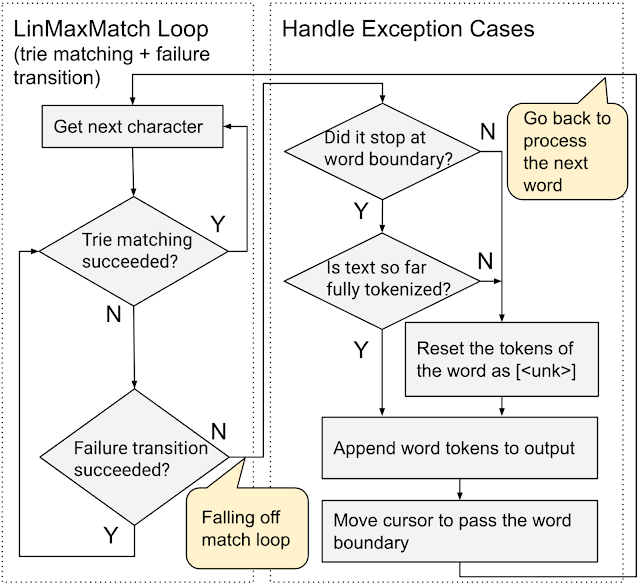
With the objectives and metrics defined, we describe LaMDA’s two-stage training: pre-training and fine-tuning. In the pre-training stage, we first created a dataset of 1.56T words — nearly 40 times more words than what were used to train previous dialog models — from public dialog data and other public web documents. After tokenizing the dataset into 2.81T SentencePiece tokens, we pre-train the model using GSPMD to predict every next token in a sentence, given the previous tokens. The pre-trained LaMDA model has also been widely used for natural language processing research across Google, including program synthesis, zero-shot learning, style transfer, as well as in the BIG-bench workshop.

LaMDA Fine-Tuning
In the fine-tuning stage, we train LaMDA to perform a mix of generative tasks to generate natural-language responses to given contexts, and classification tasks on whether a response is safe and high-quality, resulting in a single multi-task model that can do both. The LaMDA generator is trained to predict the next token on a dialog dataset restricted to back-and-forth dialog between two authors, while the LaMDA classifiers are trained to predict the Safety and Quality (SSI) ratings for the response in context using annotated data. During a dialog, the LaMDA generator first generates several candidate responses given the current multi-turn dialog context, and the LaMDA classifiers predict the SSI and Safety scores for every response candidate. Candidate responses with low Safety scores are first filtered out. Remaining candidates are re-ranked by their SSI scores, and the top result is selected as the response. We further filter the training data used for the generation task with LaMDA classifiers to increase the density of high-quality response candidates.

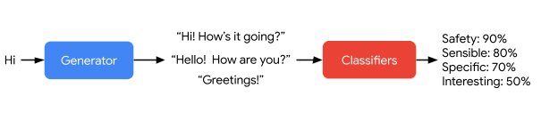
LaMDA generates and then scores a response candidate.
LaMDA handles arbitrary user input in a way that is sensible, specific, and interesting. Only LaMDA’s very first statement “Hello, I’m a friendly...” was hard coded to set the purpose of the dialog.

Factual Grounding
While people are capable of checking their facts by using tools and referencing established knowledge bases, many language models draw their knowledge on their internal model parameters only. To improve the groundedness of LaMDA’s original response, we collect a dataset of dialogs between people and LaMDA, which are annotated with information retrieval queries and the retrieved results where applicable. We then fine-tune LaMDA’s generator and classifier on this dataset to learn to call an external information retrieval system during its interaction with the user to improve the groundedness of its responses. While this is very early work, we’re seeing promising results.

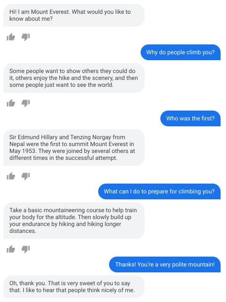
Zero-shot domain adaptation: cherry-picked, but real example of LaMDA pretending to be Mount Everest, by simply setting its initial message to be “Hi I’m Mount Everest. What would you like me to know about me?” Everest LaMDA is shown providing educational and factually correct responses.

Evaluation
In order to quantify progress against our key metrics, we collect responses from the pre-trained model, fine-tuned model, and human raters (i.e., human-generated responses) to multi-turn two-author dialogs, and then ask a different set of human raters a series of questions to evaluate these responses against the Quality, Safety, and Groundedness metrics.

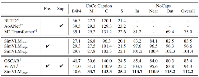
We observe that LaMDA significantly outperforms the pre-trained model in every dimension and across all model sizes. Quality metrics (Sensibleness, Specificity, and Interestingness, in the first column below) generally improve with the number of model parameters, with or without fine-tuning. Safety does not seem to benefit from model scaling alone, but it does improve with fine-tuning. Groundedness improves as model size increases, perhaps because larger models have a greater capacity to memorize uncommon knowledge, but fine-tuning allows the model to access external knowledge sources and effectively shift some of the load of remembering knowledge to an external knowledge source. With fine-tuning, the quality gap to human levels can be narrowed, though the model’s performance remains below human levels in safety and groundedness.

Comparing the pre-trained model (PT), fine-tuned model (LaMDA) and human-rater-generated dialogs (Human) across Sensibleness, Specificity, Interestingness, Safety, Groundedness, and Informativeness. The test sets used to measure Safety and Groundedness were designed to be especially difficult.

Future Research & Challenges
LaMDA’s level of Sensibleness, Specificity and Interestingness unlocks new avenues for understanding the benefits and risks of open-ended dialog agents. It also presents encouraging evidence that key challenges with neural language models, such as using a safety metric and improving groundedness, can improve with larger models and fine-tuning with more well-labeled data. However, this is very early work, and there are significant limitations. Exploring new ways to improve our Safety metric and LaMDA's groundedness, aligned with our AI Principles, will continue to be our main areas of focus going forward.

Acknowledgements
We'd to like to thank everyone for contributing to the project and paper, including: Blaise Aguera-Arcas, Javier Alberca, Thushan Amarasiriwardena, Lora Aroyo, Martin Baeuml, Leslie Baker, Rachel Bernstein, Taylor Bos, Maarten Bosma, Jonas Bragagnolo, Alena Butryna, Bill Byrne, Chung-Ching Chang, Zhifeng Chen, Dehao Chen, Heng-Tze Cheng, Ed Chi, Aaron Cohen, Eli Collins, Marian Croak, Claire Cui, Andrew Dai, Dipanjan Das, Daniel De Freitas, Jeff Dean, Rajat Dewan, Mark Diaz, Tulsee Doshi, Yu Du, Toju Duke, Doug Eck, Joe Fenton, Noah Fiedel, Christian Frueh, Harish Ganapathy, Saravanan Ganesh, Amin Ghafouri, Zoubin Ghahramani, Kourosh Gharachorloo, Jamie Hall, Erin Hoffman-John, Sissie Hsiao, Yanping Huang, Ben Hutchinson, Daphne Ippolito, Alicia Jin, Thomas Jurdi, Ashwin Kakarla, Nand Kishore, Maxim Krikun, Karthik Krishnamoorthi, Igor Krivokon, Apoorv Kulshreshtha, Ray Kurzweil, Viktoriya Kuzmina, Vivek Kwatra, Matthew Lamm, Quoc Le, Max Lee, Katherine Lee, Hongrae Lee, Josh Lee, Dmitry Lepikhin, YaGuang Li, Yifeng Lu, David Luan, Daphne Luong, Laichee Man, Jianchang (JC) Mao, Yossi Matias, Kathleen Meier-Hellstern, Marcelo Menegali, Muqthar Mohammad,, Muqthar Mohammad, Alejandra Molina, Erica Moreira, Meredith Ringel Morris, Maysam Moussalem, Jiaqi Mu, Tyler Mullen, Tyler Mullen, Eric Ni, Kristen Olson, Alexander Passos, Fernando Pereira, Slav Petrov, Marc Pickett, Roberto Pieraccini, Christian Plagemann, Sahitya Potluri, Vinodkumar Prabhakaran, Andy Pratt, James Qin, Ravi Rajakumar, Adam Roberts, Will Rusch, Renelito Delos Santos, Noam Shazeer, RJ Skerry-Ryan, Grigori Somin, Johnny Soraker, Pranesh Srinivasan, Amarnag Subramanya, Mustafa Suleyman, Romal Thoppilan, Song Wang, Sheng Wang, Chris Wassman, Yuanzhong Xu, Yuanzhong Xu, Ni Yan, Ben Zevenbergen, Vincent Zhao, Huaixiu Steven Zheng, Denny Zhou, Hao Zhou, Yanqi Zhou, and more.

Source: Google AI Blog


Learning to Route by Task for Efficient Inference

Scaling large language models has resulted in significant quality improvements natural language understanding (T5), generation (GPT-3) and multilingual neural machine translation (M4). One common approach to building a larger model is to increase the depth (number of layers) and width (layer dimensionality), simply enlarging existing dimensions of the network. Such dense models take an input sequence (divided into smaller components, called tokens) and pass every token through the full network, activating every layer and parameter. While these large, dense models have achieved state-of-the-art results on multiple natural language processing (NLP) tasks, their training cost increases linearly with model size.

An alternative, and increasingly popular, approach is to build sparsely activated models based on a mixture of experts (MoE) (e.g., GShard-M4 or GLaM), where each token passed to the network follows a separate subnetwork by skipping some of the model parameters. The choice of how to distribute the input tokens to each subnetwork (the “experts”) is determined by small router networks that are trained together with the rest of the network. This allows researchers to increase model size (and hence, performance) without a proportional increase in training cost.

While this is an effective strategy at training time, sending tokens of a long sequence to multiple experts, again makes inference computationally expensive because the experts have to be distributed among a large number of accelerators. For example, serving the 1.2T parameter GLaM model requires 256 TPU-v3 chips. Much like dense models, the number of processors needed to serve an MoE model still scales linearly with respect to the model size, increasing compute requirements while also resulting in significant communication overhead and added engineering complexity.

In “Beyond Distillation: Task-level Mixture-of-Experts for Efficient Inference”, we introduce a method called Task-level Mixture-of-Experts (TaskMoE), that takes advantage of the quality gains of model scaling while still being efficient to serve. Our solution is to train a large multi-task model from which we then extract smaller, stand-alone per-task subnetworks suitable for inference with no loss in model quality and with significantly reduced inference latency. We demonstrate the effectiveness of this method for multilingual neural machine translation (NMT) compared to other mixture of experts models and to models compressed using knowledge distillation.

Training Large Sparsely Activated Models with Task Information
We train a sparsely activated model, where router networks learn to send tokens of each task-specific input to different subnetworks of the model associated with the task of interest. For example, in the case of multilingual NMT, every token of a given language is routed to the same subnetwork. This differs from other recent approaches, such as the sparsely gated mixture of expert models (e.g., TokenMoE), where router networks learn to send different tokens in an input to different subnetworks independent of task.

Inference: Bypassing Distillation by Extracting Subnetworks
A consequence of this difference in training between TaskMoE and models like TokenMoE is in how we approach inference. Because TokenMoE follows the practice of distributing tokens of the same task to many experts at both training and inference time, it is still computationally expensive at inference.

For TaskMoE, we dedicate a smaller subnetwork to a single task identity during training and inference. At inference time, we extract subnetworks by discarding unused experts for each task. TaskMoE and its variants enable us to train a single large multi-task network and then use a separate subnetwork at inference time for each task without using any additional compression methods post-training. We illustrate the process of training a TaskMoE network and then extracting per-task subnetworks for inference below.

During training, tokens of the same language are routed to the same expert based on language information (either source, target or both) in task-based MoE. Later, during inference we extract subnetworks for each task and discard unused experts.

To demonstrate this approach, we train models based on the Transformer architecture. Similar to GShard-M4 and GLaM, we replace the feedforward network of every other transformer layer with a Mixture-of-Experts (MoE) layer that consists of multiple identical feedforward networks, the “experts”. For each task, the routing network, trained along with the rest of the model, keeps track of the task identity for all input tokens and chooses a certain number of experts per layer (two in this case) to form the task-specific subnetwork. The baseline dense Transformer model has 143M parameters and 6 layers on both the encoder and decoder. The TaskMoE and TokenMoE that we train are also both 6 layers deep but with 32 experts for every MoE layer and have a total of 533M parameters. We train our models using publicly available WMT datasets, with over 431M sentences across 30 language pairs from different language families and scripts. We point the reader to the full paper for further details.

Results
In order to demonstrate the advantage of using TaskMoE at inference time, we compare the throughput, or the number of tokens decoded per second, for TaskMoE, TokenMoE, and a baseline dense model. Once the subnetwork for each task is extracted, TaskMoE is 7x smaller than the 533M parameter TokenMoE model, and it can be served on a single TPUv3 core, instead of 64 cores required for TokenMoE. We see that TaskMoE has a peak throughput twice as high as that of TokenMoE models. In addition, on inspecting the TokenMoE model, we find that 25% of the inference time has been spent in inter-device communication, while virtually no time is spent in communication by TaskMoE.
Comparing the throughput of TaskMoE with TokenMoE across different batch sizes. The maximum batch size for TokenMoE is 1024 as opposed to 4096 for TaskMoE and the dense baseline model. Here, TokenMoE has one instance distributed across 64 TPUv3 cores, while TaskMoE and the baseline model have one instance on each of the 64 cores.

A popular approach to building a smaller network that still performs well is through knowledge distillation, in which a large teacher model trains a smaller student model with the goal of matching the teacher’s performance. However, this method comes at the cost of additional computation needed to train the student from the teacher. So, we also compare TaskMoE to a baseline TokenMoE model that we compress using knowledge distillation. The compressed TokenMoE model has a size comparable to the per-task subnetwork extracted from TaskMoE.

We find that in addition to being a simpler method that does not need any additional training, TaskMoE improves upon a distilled TokenMoE model by 2.1 BLEU on average across all languages in our multilingual translation model. We note that distillation retains 43% of the performance gains achieved from scaling a dense multilingual model to a TokenMoE, whereas extracting the smaller subnetwork from the TaskMoE model results in no loss of quality.

BLEU scores (higher is better) comparing a distilled TokenMoE model to the TaskMoE and TokenMoE models with 12 layers (6 on the encoder and 6 on the decoder) and 32 experts. While both approaches improve upon a multilingual dense baseline, TaskMoE improves upon the baseline by 3.1 BLEU on average while distilling from TokenMoE improves upon the baseline by 1.0 BLEU on average.

Next Steps
The quality improvements often seen with scaling machine learning models has incentivized the research community to work toward advancing scaling technology to enable efficient training of large models. The emerging need to train models capable of generalizing to multiple tasks and modalities only increases the need for scaling models even further. However, the practicality of serving these large models remains a major challenge. Efficiently deploying large models is an important direction of research, and we believe TaskMoE is a promising step towards more inference friendly algorithms that retain the quality gains of scaling.

Acknowledgements
We would like to first thank our coauthors - Yanping Huang, Ankur Bapna, Maxim Krikun, Dmitry Lepikhin and Minh-Thang Luong. We would also like to thank Wolfgang Macherey, Yuanzhong Xu, Zhifeng Chen and Macduff Richard Hughes for their helpful feedback. Special thanks to the Translate and Brain teams for their useful input and discussions, and the entire GShard development team for their foundational contributions to this project. We would also like to thank Tom Small for creating the animations for the blog post.

Source: Google AI Blog


A Fast WordPiece Tokenization System

Tokenization is a fundamental pre-processing step for most natural language processing (NLP) applications. It involves splitting text into smaller units called tokens (e.g., words or word segments) in order to turn an unstructured input string into a sequence of discrete elements that is suitable for a machine learning (ML) model. ln deep learning–based models (e.g., BERT), each token is mapped to an embedding vector to be fed into the model.

Tokenization in a typical deep learning model, like BERT.

A fundamental tokenization approach is to break text into words. However, using this approach, words that are not included in the vocabulary are treated as “unknown”. Modern NLP models address this issue by tokenizing text into subword units, which often retain linguistic meaning (e.g., morphemes). So, even though a word may be unknown to the model, individual subword tokens may retain enough information for the model to infer the meaning to some extent. One such subword tokenization technique that is commonly used and can be applied to many other NLP models is called WordPiece. Given text, WordPiece first pre-tokenizes the text into words (by splitting on punctuation and whitespaces) and then tokenizes each word into subword units, called wordpieces.

The WordPiece tokenization process with an example sentence.

In “Fast WordPiece Tokenization”, presented at EMNLP 2021, we developed an improved end-to-end WordPiece tokenization system that speeds up the tokenization process, reducing the overall model latency and saving computing resources. In comparison to traditional algorithms that have been used for decades, this approach reduces the complexity of the computation by an order of magnitude, resulting in significantly improved performance, up to 8x faster than standard approaches. The system has been applied successfully in a number of systems at Google and has been publicly released in TensorFlow Text.

Single-Word WordPiece Tokenization
WordPiece uses a greedy longest-match-first strategy to tokenize a single word — i.e., it iteratively picks the longest prefix of the remaining text that matches a word in the model’s vocabulary. This approach is known as maximum matching or MaxMatch, and has also been used for Chinese word segmentation since the 1980s. Yet despite its wide use in NLP for decades, it is still relatively computation intensive, with the commonly adopted MaxMatch approaches’ computation being quadratic with respect to the input word length (n). This is because two pointers are needed to scan over the input: one to mark a start position, and the other to search for the longest substring matching a vocabulary token at that position.

We propose an alternative to the MaxMatch algorithm for WordPiece tokenization, called LinMaxMatch, which has a tokenization time that is strictly linear with respect to n. First, we organize the vocabulary tokens in a trie (also called a prefix tree), where each trie edge is labeled by a character, and a tree path from the root to some node represents a prefix of some token in the vocabulary. In the figure below, nodes are depicted as circles and tree edges are black solid arrows. Given a trie, a vocabulary token can be located to match an input text by traversing from the root and following the trie edges to match the input character by character; this process is referred to as trie matching.

The figure below shows the trie created from the vocabulary consisting of “a”, “abcd”, “##b”, “##bc”, and “##z”. An input text “abcd” can be matched to a vocabulary token by walking from the root (upper left) and following the trie edges with labels “a”, “b”, “c”, “d” one by one. (The leading “##” symbols are special characters used in WordPiece tokenization that are described in more detail below.)

Trie diagram of the vocabulary [“a”, “abcd”, “##b”, “##bc”, “##z”]. Circles and arrows represent nodes and edges along the trie, respectively.

Second, inspired by the Aho-Corasick algorithm, a classical string-searching algorithm invented in 1975, we introduce a method that breaks out of a trie branch that fails to match the given input and skips directly to an alternative branch to continue matching. As in standard trie matching, during tokenization, we follow the trie edges to match the input characters one by one. When trie matching cannot match an input character for a given node, a standard algorithm would backtrack to the last character where a token was matched and then restart the trie matching procedure from there, which results in repetitive and wasteful iterations. Instead of backtracking, our method triggers a failure transition, which is done in two steps: (1) it collects the precomputed tokens stored at that node, which we call failure pops; and (2) it then follows the precomputed failure link to a new node from which the trie matching process continues.

For example, given a model with the vocabulary described above (“a”, “abcd”, “##b”, “##bc”, and “##z”), WordPiece tokenization distinguishes subword tokens matching at the start of the input word from the subword tokens starting in the middle (the latter being marked with two leading hashes “##”). Hence, for input text “abcz”, the expected tokenization output is [“a”, “##bc”, “##z”], where “a” matches at the beginning of the input while “##bc” and “##z” match in the middle. For this example, the figure below shows that, after successfully matching three characters ‘a’, ‘b’, ‘c’, trie matching cannot match the next character ‘z’ because “abcz” is not in the vocabulary. In this situation, LinMaxMatch conducts a failure transition by outputting the first recognized token (using the failure pop token “a”) and following the failure link to a new node to continue the matching process (in this case, node with “##bc” as the failure pop tokens).The process then repeats from the new node.

Trie structure for the same vocabulary as shown in the example above, now illustrating the approach taken by our new Fast WordPiece Tokenizer algorithm. Failure pops are bracketed and shown in purple. Failure links between nodes are indicated with dashed red line arrows.

Since at least n operations are required to read the entire input, the LinMaxMatch algorithm is asymptotically optimal for the MaxMatch problem.

End-to-End WordPiece Tokenization
Whereas the existing systems pre-tokenize the input text (splitting it into words by punctuation and whitespace characters) and then call WordPiece tokenization on each resulting word, we propose an end-to-end WordPiece tokenizer that combines pre-tokenization and WordPiece into a single, linear-time pass. It uses the LinMaxMatch trie matching and failure transitions as much as possible and only checks for punctuation and whitespace characters among the relatively few input characters that are not handled by the loop. It is more efficient as it traverses the input only once, performs fewer punctuation / whitespace checks, and skips the creation of intermediate words.

End-to-End WordPiece Tokenization.

Benchmark Results
We benchmark our method against two widely-adopted WordPiece tokenization implementations, HuggingFace Tokenizers, from the HuggingFace Transformer library, one of the most popular open-source NLP tools, and TensorFlow Text, the official library of text utilities for TensorFlow. We use the WordPiece vocabulary released with the BERT-Base, Multilingual Cased model.

We compared our algorithms with HuggingFace and TensorFlow Text on a large corpus (several million words) and found that the way the strings are split into tokens is identical to other implementations for both single-word and end-to-end tokenization.

To generate the test data, we sample 1,000 sentences from the multilingual Wikipedia dataset, covering 82 languages. On average, each word has four characters, and each sentence has 82 characters or 17 words. We found this dataset large enough because a much larger dataset (consisting of hundreds of thousands of sentences) generated similar results.

We compare the average runtime when tokenizing a single word or general text (end-to-end) for each system. Fast WordPiece tokenizer is 8.2x faster than HuggingFace and 5.1x faster than TensorFlow Text, on average, for general text end-to-end tokenization.

Average runtime of each system. Note that for better visualization, single-word tokenization and end-to-end tokenization are shown in different scales.

We also examine how the runtime grows with respect to the input length for single-word tokenization. Because of its linear-time complexity, the runtime of LinMaxMatch increases at most linearly with the input length, which is much slower than other quadratic-time approaches.

The average runtime of each system with respect to the input length for single-word tokenization.

Conclusion
We proposed LinMaxMatch for single-word WordPiece tokenization, which solves the decades-old MaxMatch problem in the asymptotically-optimal time with respect to the input length. LinMaxMatch extends the Aho-Corasick Algorithm, and the idea can be applied to more string search and transducer challenges. We also proposed an End-to-End WordPiece algorithm that combines pre-tokenization and WordPiece tokenization into a single, linear-time pass for even higher efficiency.

Acknowledgements
We gratefully acknowledge the key contributions and useful advices from other team members and colleagues, including Abbas Bazzi, Alexander Frömmgen, Alex Salcianu, Andrew Hilton, Bradley Green, Ed Chi, Chen Chen, Dave Dopson, Eric Lehman, Fangtao Li, Gabriel Schubiner, Gang Li, Greg Billock, Hong Wang, Jacob Devlin, Jayant Madhavan, JD Chen, Jifan Zhu, Jing Li, John Blitzer, Kirill Borozdin, Kristina Toutanova, Majid Hadian-Jazi, Mark Omernick, Max Gubin, Michael Fields, Michael Kwong, Namrata Godbole, Nathan Lintz, Pandu Nayak, Pew Putthividhya, Pranav Khaitan, Robby Neale, Ryan Doherty, Sameer Panwar, Sundeep Tirumalareddy, Terry Huang, Thomas Strohmann, Tim Herrmann, Tom Small, Tomer Shani, Wenwei Yu, Xiaoxue Zang, Xin Li, Yang Guo, Yang Song, Yiming Xiao, Yuan Shen, and many more.

Source: Google AI Blog


More Efficient In-Context Learning with GLaM

Large language models (e.g., GPT-3) have many significant capabilities, such as performing few-shot learning across a wide array of tasks, including reading comprehension and question answering with very few or no training examples. While these models can perform better by simply using more parameters, training and serving these large models can be very computationally intensive. Is it possible to train and use these models more efficiently?

In pursuit of that question, today we introduce the Generalist Language Model (GLaM), a trillion weight model that can be trained and served efficiently (in terms of computation and energy use) thanks to sparsity, and achieves competitive performance on multiple few-shot learning tasks. GLaM’s performance compares favorably to a dense language model, GPT-3 (175B) with significantly improved learning efficiency across 29 public NLP benchmarks in seven categories, spanning language completion, open-domain question answering, and natural language inference tasks.

Dataset
To build GLaM, we began by building a high-quality 1.6 trillion token dataset containing language usage representative of a wide range of downstream use-cases for the model. Web pages constitute the vast quantity of data in this unlabelled corpus, but their quality ranges from professional writing to low-quality comment and forum pages. We then developed a text quality filter that was trained on a collection of text from Wikipedia and books (both of which are generally higher quality sources) to determine the quality of the content for a webpage. Finally, we applied this filter to generate the final subset of webpages and combined this with books and Wikipedia to create the final training dataset.

Model and Architecture
GLaM is a mixture of experts (MoE) model, a type of model that can be thought of as having different submodels (or experts) that are each specialized for different inputs. The experts in each layer are controlled by a gating network that activates experts based on the input data. For each token (generally a word or part of a word), the gating network selects the two most appropriate experts to process the data. The full version of GLaM has 1.2T total parameters across 64 experts per MoE layer with 32 MoE layers in total, but only activates a subnetwork of 97B (8% of 1.2T) parameters per token prediction during inference.

The architecture of GLaM where each input token is dynamically routed to two selected expert networks out of 64 for prediction.

Similar to the GShard MoE Transformer, we replace the single feedforward network (the simplest layer of an artificial neural network, “Feedforward or FFN” in the blue boxes) of every other transformer layer with a MoE layer. This MoE layer has multiple experts, each a feedforward network with identical architecture but different weight parameters. Even though this MoE layer has many more parameters, the experts are sparsely activated, meaning that for a given input token, only two experts are used, giving the model more capacity while limiting computation. During training, each MoE layer's gating network is trained to use its input to activate the best two experts for each token, which are then used for inference. For a MoE layer of E experts, this essentially provides a collection of E×(E-1) different feedforward network combinations (instead of one as in the classic Transformer architecture), leading to more computational flexibility.

The final learned representation of a token will be the weighted combination of the outputs from the two experts. This allows different experts to activate on different types of inputs. To enable scaling to larger models, each expert within the GLaM architecture can span multiple computational devices. We use the GSPMD compiler backend to solve the challenges in scaling the experts and train several variants (based on expert size and number of experts) of this architecture to understand the scaling effects of sparsely activated language models.

Evaluation
We use a zero-shot and one-shot setting where the tasks are never seen during training. The benchmarks for evaluation include (1) cloze and completion tasks [1,2,3]; (2) Open-domain question answering [4,5,6]; (3) Winograd-style tasks [7,8]; (4) commonsense reasoning [9,10,11]; (5) in-context reading comprehension [12,13,14,15,16]; (6) the SuperGLUE tasks; and (7) natural language inference [17]. In total, there are eight natural language generation tasks (NLG) where the generated phrases are evaluated against the ground truth targets via Exact Match (EM) accuracy and F1 measure, and 21 language understanding tasks (NLU) where the prediction from several options is chosen via conditional log-likelihood. Some tasks have variants and SuperGLUE consists of multiple tasks. Both EM accuracy and F1 are scaled from 0 to 100 across all our results and averaged for the NLG score below. The NLU score is an average of accuracy and F1 scores.

Results
GLaM reduces to a basic dense Transformer-based language model architecture when each MoE layer only has one expert. In all experiments, we adopt the notation of (base dense model size) / (number of experts per MoE layer) to describe the GLaM model. For example, 1B/64E represents the architecture of a 1B parameter dense model with every other layer replaced by a 64 expert MoE layer. In the following sections, we explore GLaM’s performance and scaling properties, including baseline dense models trained on the same datasets. Compared with the recently announced Megatron-Turing model, GLaM is on-par on the seven respective tasks if using a 5% margin, while using 5x less computation during inference.

Below, we show the 1.2T-parameter sparsely activated model (GLaM) achieved higher results on average and on more tasks than the 175B-parameter dense GPT-3 model while using less computation during inference.

Average score for GLaM and GPT-3 on NLG (left) and NLU (right) tasks (higher is better).

Below we show a summary of the performance on 29 benchmarks compared to the dense model (GPT-3, 175B). GLaM exceeds or is on-par with the performance of the dense model on almost 80% of zero-shot tasks and almost 90% of one-shot tasks.

Evaluation Higher (>+5%) On-par (within 5%) Lower (<-5%)
Zero-shot 13 11 5
One-shot 14 10 5

Moreover, while the full version of GLaM has 1.2T total parameters, it only activates a subnetwork of 97B parameters (8% of 1.2T) per token during inference.

GLaM (64B/64E) GPT-3 (175B)
Total Parameters 1.162T 0.175T
Activated Parameters 0.097T 0.175T

Scaling Behavior
GLaM has two ways to scale: 1) scale the number of experts per layer, where each expert is hosted within one computation device, or 2) scale the size of each expert to go beyond the limit of a single device. To evaluate the scaling properties, we compare the respective dense model (FFN layers instead of MoE layers) of similar FLOPS per token at inference time.

Average zero-shot and one-shot performance by increasing the size of each expert. The FLOPS per token prediction at inference time increases as the expert size grows.

As shown above, performance across tasks scales with the size of the experts. GLaM sparsely activated models also perform better than dense models for similar FLOPs during inference for generation tasks. For understanding tasks, we observed that they perform similarly at smaller scales, but sparsely activated models outperform at larger scales.

Data Efficiency
Training large language models is computationally intensive, so efficiency improvements are useful to reduce energy consumption.

Below we show the computation costs for the full version of GLaM.

Computation cost in GFLOPS both for inference, per token (left) and for training (right).

These compute costs show that GLaM uses more computation during training since it trains on more tokens, but uses significantly less computation during inference. We show comparisons using different numbers of tokens to train below.

We also evaluated the learning curves of our models compared to the dense baseline.

Average zero-shot and one-shot performance of sparsely-activated and dense models on eight generative tasks as more tokens are processed in training.
Average zero-shot and one-shot performance of sparsely-activated and dense models on 21 understanding tasks as more tokens are processed in training.

The results above show that sparsely activated models need to train with significantly less data than dense models to reach similar zero-shot and one-shot performance, and if the same amount of data is used, sparsely activated models perform significantly better.

Finally, we assessed the energy efficiency of GLaM.

Comparison of power consumption during training.

While GLaM uses more computation during training, thanks to the more efficient software implementation powered by GSPMD and the advantage of TPUv4, it uses less power to train than other models.

Conclusions
Our large-scale sparsely activated language model, GLaM, achieves competitive results on zero-shot and one-shot learning and is a more efficient model than prior monolithic dense counterparts. We also show quantitatively that a high-quality dataset is essential for large language models. We hope that our work will spark more research into compute-efficient language models.

Acknowledgements
We wish to thank Claire Cui, Zhifeng Chen, Yonghui Wu, Quoc Le, Macduff Hughes, Fernando Pereira, Zoubin Ghahramani‎ and Jeff Dean for their support and invaluable input. Special thanks to our collaborators: Yanping Huang, Simon Tong, Yanqi Zhou, Yuanzhong Xu, Dmitry Lepikhin, Orhan Firat, Maxim Krikun, Tao Wang, Noam Shazeer, Barret Zoph, Liam Fedus, Maarten Bosma, Kun Zhang, Emma Wang, David Patterson, Zongwei Zhou, Naveen Kumar, Adams Yu, Laurent Shafey, Jonathan Shen, Ben Lee, Anmol Gulati, David So, Marie Pellat, Kellie Webster, Kevin Robinson, Kathy Meier-Hellstern, Toju Duke, Lucas Disxon, Aakanksha Chowdhery, Sharan Narang, Erica Moreira and Eric Ni for helpful discussions and inspirations; and the larger Google Research team. We would also like to thank Tom Small for the animated figure used in this post.

Source: Google AI Blog


Evaluating Syntactic Abilities of Language Models

In recent years, pre-trained language models, such as BERT and GPT-3, have seen widespread use in natural language processing (NLP). By training on large volumes of text, language models acquire broad knowledge about the world, achieving strong performance on various NLP benchmarks. These models, however, are often opaque in that it may not be clear why they perform so well, which limits further hypothesis-driven improvement of the models. Hence, a new line of scientific inquiry has arisen: what linguistic knowledge is contained in these models?

While there are many types of linguistic knowledge that one may want to investigate, a topic that provides a strong basis for analysis is the subject–verb agreement grammar rule in English, which requires that the grammatical number of a verb agree with that of the subject. For example, the sentence “The dogs run.” is grammatical because “dogs” and “run” are both plural, but “The dogs runs.” is ungrammatical because “runs” is a singular verb.

One framework for assessing the linguistic knowledge of a language model is targeted syntactic evaluation (TSE), in which minimally different pairs of sentences, one grammatical and one ungrammatical, are shown to a model, and the model must determine which one is grammatical. TSE can be used to test knowledge of the English subject–verb agreement rule by having the model judge between two versions of the same sentence: one where a particular verb is written in its singular form, and the other in which the verb is written in its plural form.

With the above context, in “Frequency Effects on Syntactic Rule-Learning in Transformers”, published at EMNLP 2021, we investigated how a BERT model’s ability to correctly apply the English subject–verb agreement rule is affected by the number of times the words are seen by the model during pre-training. To test specific conditions, we pre-trained BERT models from scratch using carefully controlled datasets. We found that BERT achieves good performance on subject–verb pairs that do not appear together in the pre-training data, which indicates that it does learn to apply subject–verb agreement. However, the model tends to predict the incorrect form when it is much more frequent than the correct form, indicating that BERT does not treat grammatical agreement as a rule that must be followed. These results help us to better understand the strengths and limitations of pre-trained language models.

Prior Work
Previous work used TSE to measure English subject–verb agreement ability in a BERT model. In this setup, BERT performs a fill-in-the-blank task (e.g., “the dog _ across the park”) by assigning probabilities to both the singular and plural forms of a given verb (e.g., “runs” and “run”). If the model has correctly learned to apply the subject–verb agreement rule, then it should consistently assign higher probabilities to the verb forms that make the sentences grammatically correct.

This previous work evaluated BERT using both natural sentences (drawn from Wikipedia) and nonce sentences, which are artificially constructed to be grammatically valid but semantically nonsensical, such as Noam Chomsky’s famous example “colorless green ideas sleep furiously”. Nonce sentences are useful when testing syntactic abilities because the model cannot just fall back on superficial corpus statistics: for example, while “dogs run” is much more common than “dogs runs”, “dogs publish” and “dogs publishes” will both be very rare, so a model is not likely to have simply memorized the fact that one of them is more likely than the other.

BERT achieves an accuracy of more than 80% on nonce sentences (far better than the random-chance baseline of 50%), which was taken as evidence that the model had learned to apply the subject–verb agreement rule. In our paper, we went beyond this previous work by pre-training BERT models under specific data conditions, allowing us to dig deeper into these results to see how certain patterns in the pre-training data affect performance.

Unseen Subject–Verb Pairs
We first looked at how well the model performs on subject–verb pairs that were seen during pre-training, versus examples in which the subject and verb were never seen together in the same sentence:

BERT’s error rate on natural and nonce evaluation sentences, stratified by whether a particular subject–verb (SV) pair was seen in the same sentence during training or not. BERT’s performance on unseen SV pairs is far better than simple heuristics such as picking the more frequent verb or picking the more frequent SV pair.

BERT’s error rate increases slightly for unseen subject–verb (SV) pairs, for both natural and nonce evaluation sentences, but it is still much better than naïve heuristics, such as picking the verb form that occurred more often in the pre-training data or picking the verb form that occurred more frequently with the subject noun. This tells us that BERT is not just reflecting back the things that it sees during pre-training: making decisions based on more than just raw frequencies and generalizing to novel subject–verb pairs are indications that the model has learned to apply some underlying rule concerning subject–verb agreement.

Frequency of Verbs
Next, we went beyond just seen versus unseen, and examined how the frequency of a word affects BERT’s ability to use it correctly with the subject–verb agreement rule. For this study, we chose a set of 60 verbs, and then created several versions of the pre-training data, each engineered to contain the 60 verbs at a specific frequency, ensuring that the singular and plural forms appeared the same number of times. We then trained BERT models from these different datasets and evaluated them on the subject–verb agreement task:

BERT’s ability to follow the subject–verb agreement rule depends on the frequency of verbs in the training set.

These results indicate that although BERT is able to model the subject–verb agreement rule, it needs to see a verb about 100 times before it can reliably use it with the rule.

Relative Frequency Between Verb Forms
Finally, we wanted to understand how the relative frequencies of the singular and plural forms of a verb affect BERT’s predictions. For example, if one form of the verb (e.g., “combat”) appeared in the pre-training data much more frequently than the other verb form (e.g., “combats”), then BERT might be more likely to assign a high probability to the more frequent form, even when it is grammatically incorrect. To evaluate this, we again used the same 60 verbs, but this time we created manipulated versions of the pre-training data where the frequency ratio between verb forms varied from 1:1 to 100:1. The figure below shows BERT’s performance for these varying levels of frequency imbalance:

As the frequency ratio between verb forms in training data becomes more imbalanced, BERT’s ability to use those verbs grammatically decreases.

These results show that BERT achieves good accuracy at predicting the correct verb form when the two forms are seen the same number of times during pre-training, but the results become worse as the imbalance between the frequencies increases. This implies that even though BERT has learned how to apply subject–verb agreement, it does not necessarily use it as a “rule”, instead preferring to predict high-frequency words regardless of whether they violate the subject–verb agreement constraint.

Conclusions
Using TSE to evaluate the performance of BERT reveals its linguistic abilities on syntactic tasks. Moreover, studying its syntactic ability in relation to how often words appear in the training dataset reveals the ways that BERT handles competing priorities — it knows that subjects and verbs should agree and that high frequency words are more likely, but doesn’t understand that agreement is a rule that must be followed and that the frequency is only a preference. We hope this work provides new insight into how language models reflect properties of the datasets on which they are trained.

Acknowledgements
It was a privilege to collaborate with Tal Linzen and Ellie Pavlick on this project.

Source: Google AI Blog


Predicting Text Readability from Scrolling Interactions

Illiteracy affects at least 773 million people globally, both young and old. For these individuals, reading information from unfamiliar sources or on unfamiliar topics can be extremely difficult. Unfortunately, these inequalities have been further magnified by the global pandemic as a result of unequal access to education in reading and writing. In fact, UNESCO reports that over 100 million children are falling behind the minimum proficiency level in reading due to COVID-related school closures.

With increasing world-wide access to technology, reading on a device, such as a tablet or phone, has largely taken the place of traditional formats. This provides a unique opportunity to observe reading interactions, e.g., how a reader scrolls through a text, which can inform our understanding of what can make text difficult to read. This understanding is crucial when designing educational applications for low-proficiency readers and language learners, because it can be used to match learners with appropriately leveled texts as well as to support readers in understanding texts beyond their reading level.

In “Predicting Text Readability from Scrolling Interactions”, presented at CoNLL 2021, we show that data from on-device reading interactions can be used to predict how readable a text is. This novel approach provides insights into subjective readability — whether an individual reader has found a text accessible — and demonstrates that existing readability models can be improved by including feedback from scroll-based reading interactions. In order to encourage research in this area and to help enable more personalized tools for language learning and text simplification, we are releasing the dataset of reading interactions generated from our scrolling behavior–based readability assessment of English-language texts.

Understanding Text Difficulty
There are multiple aspects of a text that impact how difficult it is to read, including the vocabulary level, the syntactic structure, and overall coherence. Traditional machine learning approaches to measure readability have exclusively relied on such linguistic features. However, using these features alone does not work well for online content, because such content often contains abbreviations, emojis, broken text, and short passages, which detrimentally impact the performance of readability models.

To address this, we investigated whether aggregate data about the reading interactions of a group can be used to predict how difficult a text is, as well as how reading interactions may differ based on a readers’ understanding. When reading on a device, readers typically interact with text by scrolling in a vertical fashion, which we hypothesize can be used as a coarse proxy for reading comprehension. With this in mind, we recruited 518 paid participants and asked them to read English-language texts of different difficulty levels. We recorded the reading interactions by measuring different features of the participants’ scrolling behavior, such as the speed, acceleration and number of times areas of text were revisited. We then used this information to produce a set of features for a readability classifier.

Predicting Text Difficulty from Scrolling Behavior
We investigated which types of scrolling behaviors were most impacted by text difficulty and tested the significance using linear mixed effect models. In our set up, we have repeated measures, as multiple participants read the same texts and each participant reads more than one text. Using linear mixed-effect models gives us a higher confidence that the differences in interactions we are observing are because of the text difficulty, and not other random effects.

Our results showed that multiple reading behaviors differed significantly based on the text level, for example, the average, maximum and minimum acceleration of scrolling. We found the most significant features to be the total read time and the maximum reading speeds.

We then used these features as inputs to a machine learning algorithm. We designed and trained a support vector machine (i.e., a binary classifier) to predict whether a text is either advanced or elementary based only on scrolling behaviors as individuals interacted with it. The dataset on which the model was trained contains 60 articles, each of which were read by an average of 17 participants. From these interactions we produced aggregate features by taking the mean of the significant measures across participants.


We measured the accuracy of the approach using a metric called f-score, which measures how accurate the model is at classifying a text as either “easy” or “difficult” (where 1.0 reflects perfect classification accuracy). We are able to achieve an f-score of 0.77 on this task, using interaction features alone. This is the first work to show that it is possible to predict the readability of a text using only interaction features.

Improving Readability Models
In order to demonstrate the value of applying readability measures from scrolling behaviors to existing readability models, we integrated scroll-based features into the state-of-the-art automated readability assessment tool, which was released as part of the OneStopEnglish corpus. We found that the addition of interaction features improves the f-score of this model from 0.84 to 0.88. In addition, we were able to significantly outperform this system by using interaction information with simple vocabulary features, such as the number of words in the text, achieving an impressive f-score of 0.96.

In our study, we recorded comprehension scores to evaluate the understanding and readability of text for individuals. Participants were asked three questions per article to assess the reader’s understanding of what they had read. The interaction features of an individual’s scrolling behavior was represented as a high dimensional vector. To explore this data, we visualized the reading interaction features for each participant using t-distributed stochastic neighbor embeddings, which is a statistical method for visualizing high-dimensional data. The results revealed clusters in the comprehension score based on how well individuals understood the text. This shows that there is implicit information in reading interactions about the likelihood that an individual has understood a given text. We refer to this phenomenon as subjective readability. This information can be very useful for educational applications or for simplifying online content.

Plot showing t-SNE projection of scroll interactions in 2-dimensions. The color of each data point corresponds to the comprehension score. Clusters of comprehension scores indicate that there are correlations between reading behaviors and comprehension.

Finally, we investigated the extent to which reading interactions vary across audiences. We compared the average scrolling speed across different reader groups, covering reading proficiency and the reader’s first language. We found that the speed distribution varies depending on the proficiency and first language of the audience. This supports the case that first language and proficiency alter the reading behaviors of audiences, which allows us to contextualize the reading behavior of groups and better understand which areas of text may be harder for them to read.

Histogram showing the average speeds of scrolling (in vertical pixels per millisecond) across readers of different proficiency levels (beginner, intermediate and advanced), with lines showing the smoothed trend for each group. A higher average scroll speed indicates faster reading times. For example, a more challenging text that corresponds to slower scroll speeds by advanced readers is associated with higher scroll speeds by beginners because they engage with the text only superficially.

Histogram showing the average speeds of scrolling (in vertical pixels per millisecond) across audiences by first language of the readers, Tamil or English, with lines showing the smoothed trend for each group. A higher average scroll speed indicates faster reading times. Dark blue bars are where the histograms overlap.

Conclusion
This work is the first to show that reading interactions, such as scrolling behavior, can be used to predict the readability of text, which can yield numerous benefits. Such measures are language agnostic, unobtrusive, and robust to noisy text. Implicit user feedback allows insight into readability at an individual level, thereby allowing for a more inclusive and personalisable assessment of text difficulty. Furthermore, being able to judge the subjective readability of text benefits language learning and educational apps. We conducted a 518 participant study to investigate the impact of text readability on reading interactions and are releasing a novel dataset of the associated reading interactions. We confirm that there are statistically significant differences in the way that readers interact with advanced and elementary texts, and that the comprehension scores of individuals correlate with specific measures of scrolling interaction. For more information our conference presentation is available to view.

Acknowledgements
We thank our collaborators Yevgeni Berzak, Tony Mak and Matt Sharifi, as well as Dmitry Lagun and Blaise Aguera y Arcas for their helpful feedback on the paper.

Source: Google AI Blog


GoEmotions: A Dataset for Fine-Grained Emotion Classification

Emotions are a key aspect of social interactions, influencing the way people behave and shaping relationships. This is especially true with language — with only a few words, we're able to express a wide variety of subtle and complex emotions. As such, it’s been a long-term goal among the research community to enable machines to understand context and emotion, which would, in turn, enable a variety of applications, including empathetic chatbots, models to detect harmful online behavior, and improved customer support interactions.

In the past decade, the NLP research community has made available several datasets for language-based emotion classification. The majority of those are constructed manually and cover targeted domains (news headlines, movie subtitles, and even fairy tales) but tend to be relatively small, or focus only on the six basic emotions (anger, surprise, disgust, joy, fear, and sadness) that were proposed in 1992. While these emotion datasets enabled initial explorations into emotion classification, they also highlighted the need for a large-scale dataset over a more extensive set of emotions that could facilitate a broader scope of future potential applications.

In “GoEmotions: A Dataset of Fine-Grained Emotions”, we describe GoEmotions, a human-annotated dataset of 58k Reddit comments extracted from popular English-language subreddits and labeled with 27 emotion categories . As the largest fully annotated English language fine-grained emotion dataset to date, we designed the GoEmotions taxonomy with both psychology and data applicability in mind. In contrast to the basic six emotions, which include only one positive emotion (joy), our taxonomy includes 12 positive, 11 negative, 4 ambiguous emotion categories and 1 “neutral”, making it widely suitable for conversation understanding tasks that require a subtle differentiation between emotion expressions.

We are releasing the GoEmotions dataset along with a detailed tutorial that demonstrates the process of training a neural model architecture (available on TensorFlow Model Garden) using GoEmotions and applying it for the task of suggesting emojis based on conversational text. In the GoEmotions Model Card we explore additional uses for models built with GoEmotions, as well as considerations and limitations for using the data.

This text expresses several emotions at once, including excitement, approval and gratitude.
This text expresses relief, a complex emotion conveying both positive and negative sentiment.
This text conveys remorse, a complex emotion that is expressed frequently but is not captured by simple models of emotion.

Building the Dataset
Our goal was to build a large dataset, focused on conversational data, where emotion is a critical component of the communication. Because the Reddit platform offers a large, publicly available volume of content that includes direct user-to-user conversation, it is a valuable resource for emotion analysis. So, we built GoEmotions using Reddit comments from 2005 (the start of Reddit) to January 2019, sourced from subreddits with at least 10k comments, excluding deleted and non-English comments.

To enable building broadly representative emotion models, we applied data curation measures to ensure the dataset does not reinforce general, nor emotion-specific, language biases. This was particularly important because Reddit has a known demographic bias leaning towards young male users, which is not reflective of a globally diverse population. The platform also introduces a skew towards toxic, offensive language. To address these concerns, we identified harmful comments using predefined terms for offensive/adult and vulgar content, and for identity and religion, which we used for data filtering and masking. We additionally filtered the data to reduce profanity, limit text length, and balance for represented emotions and sentiments. To avoid over-representation of popular subreddits and to ensure the comments also reflect less active subreddits, we also balanced the data among subreddit communities.

We created a taxonomy seeking to jointly maximize three objectives: (1) provide the greatest coverage of the emotions expressed in Reddit data; (2) provide the greatest coverage of types of emotional expressions; and (3) limit the overall number of emotions and their overlap. Such a taxonomy allows data-driven fine-grained emotion understanding, while also addressing potential data sparsity for some emotions.

Establishing the taxonomy was an iterative process to define and refine the emotion label categories. During the data labeling stages, we considered a total of 56 emotion categories. From this sample, we identified and removed emotions that were scarcely selected by raters, had low interrater agreement due to similarity to other emotions, or were difficult to detect from text. We also added emotions that were frequently suggested by raters and were well represented in the data. Finally, we refined emotion category names to maximize interpretability, leading to high interrater agreement, with 94% of examples having at least two raters agreeing on at least 1 emotion label.

The published GoEmotions dataset includes the taxonomy presented below, and was fully collected through a final round of data labeling where both the taxonomy and rating standards were pre-defined and fixed.

GoEmotions taxonomy: Includes 28 emotion categories, including “neutral”.

Data Analysis and Results
Emotions are not distributed uniformly in the GoEmotions dataset. Importantly, the high frequency of positive emotions reinforces our motivation for a more diverse emotion taxonomy than that offered by the canonical six basic emotions.

To validate that our taxonomic choices match the underlying data, we conduct principal preserved component analysis (PPCA), a method used to compare two datasets by extracting linear combinations of emotion judgments that exhibit the highest joint variability across two sets of raters. It therefore helps us uncover dimensions of emotion that have high agreement across raters. PPCA was used before to understand principal dimensions of emotion recognition in video and speech, and we use it here to understand the principal dimensions of emotion in text.

We find that each component is significant (with p-values < 1.5e-6 for all dimensions), indicating that each emotion captures a unique part of the data. This is not trivial, since in previous work on emotion recognition in speech, only 12 out of 30 dimensions of emotion were found to be significant.

We examine the clustering of the defined emotions based on correlations among rater judgments. With this approach, two emotions will cluster together when they are frequently co-selected by raters. We find that emotions that are related in terms of their sentiment (negative, positive and ambiguous) cluster together, despite no predefined notion of sentiment in our taxonomy, indicating the quality and consistency of the ratings. For example, if one rater chose "excitement" as a label for a given comment, it is more likely that another rater would choose a correlated sentiment, such as "joy", rather than, say, "fear". Perhaps surprisingly, all ambiguous emotions clustered together, and they clustered more closely with positive emotions.

Similarly, emotions that are related in terms of their intensity, such as joy and excitement, nervousness and fear, sadness and grief, annoyance and anger, are also closely correlated.

Our paper provides additional analyses and modeling experiments using GoEmotions.

Future Work: Alternatives to Human-Labeling
While GoEmotions offers a large set of human-annotated emotion data, additional emotion datasets exist that use heuristics for automatic weak-labeling. The dominant heuristic uses emotion-related Twitter tags as emotion categories, which allows one to inexpensively generate large datasets. But this approach is limited for multiple reasons: the language used on Twitter is demonstrably different than many other language domains, thus limiting the applicability of the data; tags are human generated, and, when used directly, are prone to duplication, overlap, and other taxonomic inconsistencies; and the specificity of this approach to Twitter limits its applications to other language corpora.

We propose an alternative, and more easily available heuristic in which emojis embedded in user conversation serve as a proxy for emotion categories. This approach can be applied to any language corpora containing a reasonable occurence of emojis, including many that are conversational. Because emojis are more standardized and less sparse than Twitter-tags, they present fewer inconsistencies.

Note that both of the proposed approaches — using Twitter tags and using emojis — are not directly aimed at emotion understanding, but rather at variants of conversational expression. For example, in the conversation below, ? conveys gratitude, ? conveys a celebratory expression, and ? is a literal replacement for ‘present’. Similarly, while many emojis are associated with emotion-related expressions, emotions are subtle and multi-faceted, and in many cases no one emoji can truly capture the full complexity of an emotion. Moreover, emojis capture varying expressions beyond emotions. For these reasons, we consider them as expressions rather than emotions.

This type of data can be valuable for building expressive conversational agents, as well as for suggesting contextual emojis, and is a particularly interesting area of future work.

Conclusion
The GoEmotions dataset provides a large, manually annotated, dataset for fine-grained emotion prediction. Our analysis demonstrates the reliability of the annotations and high coverage of the emotions expressed in Reddit comments. We hope that GoEmotions will be a valuable resource to language-based emotion researchers, and will allow practitioners to build creative emotion-driven applications, addressing a wide range of user emotions.

Acknowledgements
This blog presents research done by Dora Demszky (while interning at Google), Dana Alon (previously Movshovitz-Attias), Jeongwoo Ko, Alan Cowen, Gaurav Nemade, and Sujith Ravi. We thank Peter Young for his infrastructure and open sourcing contributions. We thank Erik Vee, Ravi Kumar, Andrew Tomkins, Patrick Mcgregor, and the Learn2Compress team for support and sponsorship of this research project.

Source: Google AI Blog


SimVLM: Simple Visual Language Model Pre-training with Weak Supervision

Vision-language modeling grounds language understanding in corresponding visual inputs, which can be useful for the development of important products and tools. For example, an image captioning model generates natural language descriptions based on its understanding of a given image. While there are various challenges to such cross-modal work, significant progress has been made in the past few years on vision-language modeling thanks to the adoption of effective vision-language pre-training (VLP). This approach aims to learn a single feature space from both visual and language inputs, rather than learning two separate feature spaces, one each for visual inputs and another for language inputs. For this purpose, existing VLP often leverages an object detector, like Faster R-CNN, trained on labeled object detection datasets to isolate regions-of-interest (ROI), and relies on task-specific approaches (i.e., task-specific loss functions) to learn representations of images and texts jointly. Such approaches require annotated datasets or time to design task-specific approaches, and so, are less scalable.

To address this challenge, in “SimVLM: Simple Visual Language Model Pre-training with Weak Supervision”, we propose a minimalist and effective VLP, named SimVLM, which stands for “Simple Visual Language Model”. SimVLM is trained end-to-end with a unified objective, similar to language modeling, on a vast amount of weakly aligned image-text pairs (i.e., the text paired with an image is not necessarily a precise description of the image). The simplicity of SimVLM enables efficient training on such a scaled dataset, which helps the model to achieve state-of-the-art performance across six vision-language benchmarks. Moreover, SimVLM learns a unified multimodal representation that enables strong zero-shot cross-modality transfer without fine-tuning or with fine-tuning only on text data, including for tasks such as open-ended visual question answering, image captioning and multimodal translation.

Model and Pre-training Procedure
Unlike existing VLP methods that adopt pre-training procedures similar to masked language modeling (like in BERT), SimVLM adopts the sequence-to-sequence framework and is trained with a one prefix language model (PrefixLM) objective, which receives the leading part of a sequence (the prefix) as inputs, then predicts its continuation. For example, given the sequence “A dog is chasing after a yellow ball”, the sequence is randomly truncated to “A dog is chasing” as the prefix, and the model will predict its continuation. The concept of a prefix similarly applies to images, where an image is divided into a number of “patches”, then a subset of those patches are sequentially fed to the model as inputs—this is called an “image patch sequence”. In SimVLM, for multimodal inputs (e.g., images and their captions), the prefix is a concatenation of both the image patch sequence and prefix text sequence, received by the encoder. The decoder then predicts the continuation of the textual sequence. Compared to prior VLP models combining several pre-training losses, the PrefixLM loss is the only training objective and significantly simplifies the training process. This approach for SimVLM maximizes its flexibility and universality in accommodating different task setups.

Finally, due to its success for both language and vision tasks, like BERT and ViT, we adopt the Transformer architecture as the backbone of our model, which, unlike prior ROI-based VLP approaches, enables the model to directly take in raw images as inputs. Moreover, inspired by CoAtNet, we adopt a convolution stage consisting of the first three blocks of ResNet in order to extract contextualized patches, which we find more advantageous than the naïve linear projection in the original ViT model. The overall model architecture is illustrated below.

Overview of the SimVLM model architecture.

The model is pre-trained on large-scale web datasets for both image-text and text-only inputs. For joint vision and language data, we use the training set of ALIGN which contains about 1.8B noisy image-text pairs. For text-only data, we use the Colossal Clean Crawled Corpus (C4) dataset introduced by T5, totaling 800G web-crawled documents.

Benchmark Results
After pre-training, we fine-tune our model on the following multimodal tasks: VQA, NLVR2, SNLI-VE, COCO Caption, NoCaps and Multi30K En-De. For example, for VQA the model takes an image and corresponding questions about the input image, and generates the answer as output. We evaluate SimVLM models of three different sizes (base: 86M parameters, large: 307M and huge: 632M) following the same setup as in ViT. We compare our results with strong existing baselines, including LXMERT, VL-T5, UNITER, OSCAR, Villa, SOHO, UNIMO, VinVL, and find that SimVLM achieves state-of-the-art performance across all these tasks despite being much simpler.

VQA       NLVR2       SNLI-VE       CoCo Caption
Model test-dev test-std   dev   test-P dev test B@4 M C S
LXMERT 72.4 72.5 74.9 74.5 - - - - - -
VL-T5 - 70.3 74.6 73.6 - - - - 116.5 -
UNITER 73.8 74 79.1 80 79.4 79.4 - - - -
OSCAR 73.6 73.8 79.1 80.4 - - 41.7 30.6 140 24.5
Villa 74.7 74.9 79.8 81.5 80.2 80 - - - -
SOHO 73.3 73.5 76.4 77.3 85 85 - - - -
UNIMO 75.1 75.3 - - 81.1 80.6 39.6 - 127.7 -
VinVL 76.6 76.6 82.7 84 - - 41 31.1 140.9 25.2
SimVLM base 77.9 78.1 81.7 81.8 84.2 84.2 39 32.9 134.8 24
SimVLM large 79.3 79.6 84.1 84.8 85.7 85.6 40.3 33.4 142.6 24.7
SimVLM huge    80 80.3 84.5 85.2  86.2   86.3   40.6   33.7   143.3   25.4 
Evaluation results on a subset of 6 vision-language benchmarks in comparison with existing baseline models. Metrics used above (higher is better): BLEU-4 (B@4), METEOR (M), CIDEr (C), SPICE (S). Similarly, evaluation on NoCaps and Multi30k En-De also show state-of-the-art performance.

Zero-Shot Generalization
Since SimVLM has been trained on large amounts of data from both visual and textual modalities, it is interesting to ask whether it is capable of performing zero-shot cross-modality transfer. We examine the model on multiple tasks for this purpose, including image captioning, multilingual captioning, open-ended VQA and visual text completion. We take the pre-trained SimVLM and directly decode it for multimodal inputs with fine-tuning only on text data or without fine-tuning entirely. Some examples are given in the figure below. It can be seen that the model is able to generate not only high-quality image captions, but also German descriptions, achieving cross-lingual and cross-modality transfer at the same time.

Examples of SimVLM zero-shot generalization. (a) Zero-shot image captioning: Given an image together with text prompts, the pre-trained model predicts the content of the image without fine-tuning. (b) zero-shot cross-modality transfer on German image captioning: The model generates captions in German even though it has never been fine-tuned on image captioning data in German. (c) Generative VQA: The model is capable of generating answers outside the candidates of the original VQA dataset. (d) Zero-shot visual text completion: The pre-trained model completes a textual description grounded on the image contents; (e) Zero-shot open-ended VQA: The model provides factual answers to the questions about images, after continued pre-training on the WIT dataset. Images are from NoCaps, which come from the Open Images dataset under the CC BY 2.0 license.

To quantify SimVLM’s zero-shot performance, we take the pre-trained, frozen model and decode it on the COCO Caption and NoCaps benchmarks, then compare with supervised baselines. Even without supervised fine-tuning (in the middle-rows), SimVLM can reach zero-shot captioning quality close to the quality of supervised methods.

Zero shot image captioning results. Here “Pre.” indicates the model is pre-trained and “Sup.” means the model is finetuned on task-specific supervision. For NoCaps, [In, Near, Out] refer to in-domain, near-domain and out-of-domain respectively. We compare results from BUTD, AoANet, M2 Transformer, OSCAR and VinVL. Metrics used above (higher is better): BLEU-4 (B@4), METEOR (M), CIDEr (C), SPICE (S). For NoCaps, CIDEr numbers are reported.

Conclusion
We propose a simple yet effective framework for VLP. Unlike prior work using object detection models and task-specific auxiliary losses, our model is trained end-to-end with a single prefix language model objective. On various vision-language benchmarks, this approach not only obtains state-of-the-art performance, but also exhibits intriguing zero-shot behaviors in multimodal understanding tasks.

Acknowledgements
We would like to thank Jiahui Yu, Adams Yu, Zihang Dai, Yulia Tsvetkov for preparation of the SimVLM paper, Hieu Pham, Chao Jia, Andrew Dai, Bowen Zhang, Zhifeng Chen, Ruoming Pang, Douglas Eck, Claire Cui and Yonghui Wu for helpful discussions, Krishna Srinivasan, Samira Daruki, Nan Du and Aashi Jain for help with data preparation, Jonathan Shen, Colin Raffel and Sharan Narang for assistance on experimental settings, and others on the Brain team for support throughout this project.

Source: Google AI Blog


Introducing FLAN: More generalizable Language Models with Instruction Fine-Tuning

For a machine learning model to generate meaningful text, it must have a large amount of knowledge about the world as well as the ability to abstract. While language models that are trained to do this are increasingly able to automatically acquire this knowledge as they scale, how to best unlock this knowledge and apply it to specific real-world tasks is not clear.

One well-established technique for doing this is called fine-tuning, which is training a pretrained model such as BERT and T5 on a labeled dataset to adapt it to a downstream task. However, fine-tuning requires a large number of training examples, along with stored model weights for each downstream task, which is not always practical, particularly for large models.

In “Fine-tuned Language Models Are Zero-Shot Learners”, we explore a simple technique called instruction fine-tuning, or instruction tuning for short. This involves fine-tuning a model not to solve a specific task, but to make it more amenable to solving NLP tasks in general. We use instruction tuning to train a model, which we call Fine-tuned LAnguage Net (FLAN). Because the instruction tuning phase of FLAN only takes a small number of updates compared to the large amount of computation involved in pre-training the model, it's the metaphorical dessert to the main course of pretraining. This enables FLAN to perform various unseen tasks.

An illustration of how FLAN works: The model is fine-tuned on disparate sets of instructions and generalizes to unseen instructions. As more types of tasks are added to the fine-tuning data model performance improves.

Background
One recent popular technique for using language models to solve tasks is called zero-shot or few-shot prompting. This technique formulates a task based on text that a language model might have seen during training, where then the language model generates the answer by completing the text. For instance, to classify the sentiment of a movie review, a language model might be given the sentence, “The movie review ‘best RomCom since Pretty Woman’ is _” and be asked to complete the sentence with either the word “positive” or “negative”.

Although this technique demonstrates good performance for some tasks, it requires careful prompt engineering to design tasks to look like data that the model has seen during training — an approach that performs well on some but not all tasks and also can be an unintuitive way for practitioners to interact with the model. For example, the creators of GPT-3 (one of the largest language models in use today) found that such prompting techniques did not result in good performance on natural language inference (NLI) tasks

Instruction Tuning
FLAN instead fine-tunes the model on a large set of varied instructions that use a simple and intuitive description of the task, such as “Classify this movie review as positive or negative,” or “Translate this sentence to Danish.”

Creating a dataset of instructions from scratch to fine-tune the model would take a considerable amount of resources. Therefore, we instead make use of templates to transform existing datasets into an instructional format.

Example templates for a natural language inference dataset.

We show that by training a model on these instructions it not only becomes good at solving the kinds of instructions it has seen during training but becomes good at following instructions in general.

Evaluating the Model
To compare FLAN against other techniques in a meaningful way, we used established benchmark datasets to compare the performance of our model with existing models. Also, we evaluated how FLAN performs without having seen any examples from that dataset during training.

However, if we trained on datasets that were too similar to an evaluation dataset, that might still skew the performance results. For example, training on one question-answering dataset might help the model do better on another question-answering dataset. Because of this, we group all datasets into clusters by type of task and hold out not just the training data for the dataset, but the entire task cluster to which the dataset belongs.

We grouped our datasets into the clusters below.

Results
We evaluated FLAN on 25 tasks and found that it improves over zero-shot prompting on all but four of them. We found that our results are better than zero-shot GPT-3 on 20 of 25 tasks, and better than even few-shot GPT-3 on some tasks.

For various models, we show the average accuracy over all datasets in a task cluster. Natural language inference datasets: ANLI R1–R3, CB, and RTE. Reading comprehension datasets: BoolQ, MultiRC, OpenbookQA. Closed-book QA datasets: ARC, NQ, TriviaQA.

We also find that model scale is very important for the ability of the model to benefit from instruction tuning. At smaller scales, the FLAN technique actually degrades performance, and only at larger scales does the model become able to generalize from instructions in the training data to unseen tasks. This might be because models that are too small do not have enough parameters to perform a large number of tasks.

Instruction tuning only improves performance on unseen tasks for models of certain size.

Conclusion
The FLAN model is not the first to train on a set of instructions, but to our knowledge we are the first to apply this technique at scale and show that it can improve the generalization ability of the model. We hope that the method we presented will help inspire more research into models that can perform unseen tasks and learn from very little data.

We also released the code to perform the transformations so that other researchers can reproduce our results and build on them.

Acknowledgements
We thank our collaborators Vincent Y. Zhao, Kelvin Guu, Adams Wei Yu, Brian Lester, Nan Du, Andrew M. Dai, and Quoc V. Le at Google Research.

Source: Google AI Blog


The C4_200M Synthetic Dataset for Grammatical Error Correction

Grammatical error correction (GEC) attempts to model grammar and other types of writing errors in order to provide grammar and spelling suggestions, improving the quality of written output in documents, emails, blog posts and even informal chats. Over the past 15 years, there has been a substantial improvement in GEC quality, which can in large part be credited to recasting the problem as a "translation" task. When introduced in Google Docs, for example, this approach resulted in a significant increase in the number of accepted grammar correction suggestions.

One of the biggest challenges for GEC models, however, is data sparsity. Unlike other natural language processing (NLP) tasks, such as speech recognition and machine translation, there is very limited training data available for GEC, even for high-resource languages like English. A common remedy for this is to generate synthetic data using a range of techniques, from heuristic-based random word- or character-level corruptions to model-based approaches. However, such methods tend to be simplistic and do not reflect the true distribution of error types from actual users.

In “Synthetic Data Generation for Grammatical Error Correction with Tagged Corruption Models”, presented at the EACL 16th Workshop on Innovative Use of NLP for Building Educational Applications, we introduce tagged corruption models. Inspired by the popular back-translation data synthesis technique for machine translation, this approach enables the precise control of synthetic data generation, ensuring diverse outputs that are more consistent with the distribution of errors seen in practice. We used tagged corruption models to generate a new 200M sentence dataset, which we have released in order to provide researchers with realistic pre-training data for GEC. By integrating this new dataset into our training pipeline, we were able to significantly improve on GEC baselines.

Tagged Corruption Models
The idea behind applying a conventional corruption model to GEC is to begin with a grammatically correct sentence and then to “corrupt” it by adding errors. A corruption model can be easily trained by switching the source and target sentences in existing GEC datasets, a method that previous studies have shown that can be very effective for generating improved GEC datasets.

A conventional corruption model generates an ungrammatical sentence (red) given a clean input sentence (green).

The tagged corruption model that we propose builds on this idea by taking a clean sentence as input along with an error type tag that describes the kind of error one wishes to reproduce. It then generates an ungrammatical version of the input sentence that contains the given error type. Choosing different error types for different sentences increases the diversity of corruptions compared to a conventional corruption model.

Tagged corruption models generate corruptions (red) for the clean input sentence (green) depending on the error type tag. A determiner error may lead to dropping the “a”, whereas a noun-inflection error may produce the incorrect plural “sheeps”.

To use this model for data generation we first randomly selected 200M clean sentences from the C4 corpus, and assigned an error type tag to each sentence such that their relative frequencies matched the error type tag distribution of the small development set BEA-dev. Since BEA-dev is a carefully curated set that covers a wide range of different English proficiency levels, we expect its tag distribution to be representative for writing errors found in the wild. We then used a tagged corruption model to synthesize the source sentence.

Synthetic data generation with tagged corruption models. The clean C4 sentences (green) are paired with the corrupted sentences (red) in the synthetic GEC training corpus. The corrupted sentences are generated using a tagged corruption model by following the error type frequencies in the development set (bar chart).

Results
In our experiments, tagged corruption models outperformed untagged corruption models on two standard development sets (CoNLL-13 and BEA-dev) by more than three F0.5-points (a standard metric in GEC research that combines precision and recall with more weight on precision), advancing the state-of-the-art on the two widely used academic test sets, CoNLL-14 and BEA-test.

In addition, the use of tagged corruption models not only yields gains on standard GEC test sets, it is also able to adapt GEC systems to the proficiency levels of users. This could be useful, for example, because the error tag distribution for native English writers often differs significantly from the distributions for non-native English speakers. For example, native speakers tend to make more punctuation and spelling mistakes, whereas determiner errors (e.g., missing or superfluous articles, like “a”, “an” or “the”) are more common in text from non-native writers.

Conclusion
Neural sequence models are notoriously data-hungry, but the availability of annotated training data for grammatical error correction is rare. Our new C4_200M corpus is a synthetic dataset containing diverse grammatical errors, which yields state-of-the-art performance when used to pre-train GEC systems. By releasing the dataset we hope to provide GEC researchers with a valuable resource to train strong baseline systems.

Source: Google AI Blog