Tag Archives: machine learning

World scale inverse reinforcement learning in Google Maps

Posted by Matt Barnes, Software Engineer, Google Research

Routing in Google Maps remains one of our most helpful and frequently used features. Determining the best route from A to B requires making complex trade-offs between factors including the estimated time of arrival (ETA), tolls, directness, surface conditions (e.g., paved, unpaved roads), and user preferences, which vary across transportation mode and local geography. Often, the most natural visibility we have into travelers' preferences is by analyzing real-world travel patterns.

Learning preferences from observed sequential decision making behavior is a classic application of inverse reinforcement learning (IRL). Given a Markov decision process (MDP) — a formalization of the road network — and a set of demonstration trajectories (the traveled routes), the goal of IRL is to recover the users' latent reward function. Although past research has created increasingly general IRL solutions, these have not been successfully scaled to world-sized MDPs. Scaling IRL algorithms is challenging because they typically require solving an RL subroutine at every update step. At first glance, even attempting to fit a world-scale MDP into memory to compute a single gradient step appears infeasible due to the large number of road segments and limited high bandwidth memory. When applying IRL to routing, one needs to consider all reasonable routes between each demonstration's origin and destination. This implies that any attempt to break the world-scale MDP into smaller components cannot consider components smaller than a metropolitan area.

To this end, in "Massively Scalable Inverse Reinforcement Learning in Google Maps", we share the result of a multi-year collaboration among Google Research, Maps, and Google DeepMind to surpass this IRL scalability limitation. We revisit classic algorithms in this space, and introduce advances in graph compression and parallelization, along with a new IRL algorithm called Receding Horizon Inverse Planning (RHIP) that provides fine-grained control over performance trade-offs. The final RHIP policy achieves a 16–24% relative improvement in global route match rate, i.e., the percentage of de-identified traveled routes that exactly match the suggested route in Google Maps. To the best of our knowledge, this represents the largest instance of IRL in a real world setting to date.

Google Maps improvements in route match rate relative to the existing baseline, when using the RHIP inverse reinforcement learning policy.

The benefits of IRL

A subtle but crucial detail about the routing problem is that it is goal conditioned, meaning that every destination state induces a slightly different MDP (specifically, the destination is a terminal, zero-reward state). IRL approaches are well suited for these types of problems because the learned reward function transfers across MDPs, and only the destination state is modified. This is in contrast to approaches that directly learn a policy, which typically require an extra factor of S parameters, where S is the number of MDP states.

Once the reward function is learned via IRL, we take advantage of a powerful inference-time trick. First, we evaluate the entire graph's rewards once in an offline batch setting. This computation is performed entirely on servers without access to individual trips, and operates only over batches of road segments in the graph. Then, we save the results to an in-memory database and use a fast online graph search algorithm to find the highest reward path for routing requests between any origin and destination. This circumvents the need to perform online inference of a deeply parameterized model or policy, and vastly improves serving costs and latency.

Reward model deployment using batch inference and fast online planners.

Receding Horizon Inverse Planning

To scale IRL to the world MDP, we compress the graph and shard the global MDP using a sparse Mixture of Experts (MoE) based on geographic regions. We then apply classic IRL algorithms to solve the local MDPs, estimate the loss, and send gradients back to the MoE. The worldwide reward graph is computed by decompressing the final MoE reward model. To provide more control over performance characteristics, we introduce a new generalized IRL algorithm called Receding Horizon Inverse Planning (RHIP).

IRL reward model training using MoE parallelization, graph compression, and RHIP.

RHIP is inspired by people’s tendency to perform extensive local planning ("What am I doing for the next hour?") and approximate long-term planning ("What will my life look like in 5 years?"). To take advantage of this insight, RHIP uses robust yet expensive stochastic policies in the local region surrounding the demonstration path, and switches to cheaper deterministic planners beyond some horizon. Adjusting the horizon H allows controlling computational costs, and often allows the discovery of the performance sweet spot. Interestingly, RHIP generalizes many classic IRL algorithms and provides the novel insight that they can be viewed along a stochastic vs. deterministic spectrum (specifically, for H=∞ it reduces to MaxEnt, for H=1 it reduces to BIRL, and for H=0 it reduces to MMP).

Given a demonstration from s_o to s_d, (1) RHIP follows a robust yet expensive stochastic policy in the local region surrounding the demonstration (blue region). (2) Beyond some horizon H, RHIP switches to following a cheaper deterministic planner (red lines). Adjusting the horizon enables fine-grained control over performance and computational costs.

Routing wins

The RHIP policy provides a 15.9% and 24.1% lift in global route match rate for driving and two-wheelers (e.g., scooters, motorcycles, mopeds) relative to the well-tuned Maps baseline, respectively. We're especially excited about the benefits to more sustainable transportation modes, where factors beyond journey time play a substantial role. By tuning RHIP's horizon H, we're able to achieve a policy that is both more accurate than all other IRL policies and 70% faster than MaxEnt.

Our 360M parameter reward model provides intuitive wins for Google Maps users in live A/B experiments. Examining road segments with a large absolute difference between the learned rewards and the baseline rewards can help improve certain Google Maps routes. For example:

Nottingham, UK. The preferred route (blue) was previously marked as private property due to the presence of a large gate, which indicated to our systems that the road may be closed at times and would not be ideal for drivers. As a result, Google Maps routed drivers through a longer, alternate detour instead (red). However, because real-world driving patterns showed that users regularly take the preferred route without an issue (as the gate is almost never closed), IRL now learns to route drivers along the preferred route by placing a large positive reward on this road segment.

Conclusion

Increasing performance via increased scale – both in terms of dataset size and model complexity – has proven to be a persistent trend in machine learning. Similar gains for inverse reinforcement learning problems have historically remained elusive, largely due to the challenges with handling practically sized MDPs. By introducing scalability advancements to classic IRL algorithms, we're now able to train reward models on problems with hundreds of millions of states, demonstration trajectories, and model parameters, respectively. To the best of our knowledge, this is the largest instance of IRL in a real-world setting to date. See the paper to learn more about this work.

Acknowledgements

This work is a collaboration across multiple teams at Google. Contributors to the project include Matthew Abueg, Oliver Lange, Matt Deeds, Jason Trader, Denali Molitor, Markus Wulfmeier, Shawn O'Banion, Ryan Epp, Renaud Hartert, Rui Song, Thomas Sharp, Rémi Robert, Zoltan Szego, Beth Luan, Brit Larabee and Agnieszka Madurska.

We’d also like to extend our thanks to Arno Eigenwillig, Jacob Moorman, Jonathan Spencer, Remi Munos, Michael Bloesch and Arun Ahuja for valuable discussions and suggestions.

Source: Google AI Blog

A novel computational fluid dynamics framework for turbulent flow research

Posted by Shantanu Shahane, Software Engineer, and Matthias Ihme, Research Scientist, Athena Team

Turbulence is ubiquitous in environmental and engineering fluid flows, and is encountered routinely in everyday life. A better understanding of these turbulent processes could provide valuable insights across a variety of research areas — improving the prediction of cloud formation by atmospheric transport and the spreading of wildfires by turbulent energy exchange, understanding sedimentation of deposits in rivers, and improving the efficiency of combustion in aircraft engines to reduce emissions, to name a few. However, despite its importance, our current understanding and our ability to reliably predict such flows remains limited. This is mainly attributed to the highly chaotic nature and the enormous spatial and temporal scales these fluid flows occupy, ranging from energetic, large-scale movements on the order of several meters on the high-end, where energy is injected into the fluid flow, all the way down to micrometers (μm) on the low-end, where the turbulence is dissipated into heat by viscous friction.

A powerful tool to understand these turbulent flows is the direct numerical simulation (DNS), which provides a detailed representation of the unsteady three-dimensional flow-field without making any approximations or simplifications. More specifically, this approach utilizes a discrete grid with small enough grid spacing to capture the underlying continuous equations that govern the dynamics of the system (in this case, variable-density Navier-Stokes equations, which govern all fluid flow dynamics). When the grid spacing is small enough, the discrete grid points are enough to represent the true (continuous) equations without the loss of accuracy. While this is attractive, such simulations require tremendous computational resources in order to capture the correct fluid-flow behaviors across such a wide range of spatial scales.

The actual span in spatial resolution to which direct numerical calculations must be applied depends on the task and is determined by the Reynolds number, which compares inertial to viscous forces. Typically, the Reynolds number can range between 10² up to 10⁷(even larger for atmospheric or interstellar problems). In 3D, the grid size for the resolution required scales roughly with the Reynolds number to the power of 4.5! Because of this strong scaling dependency, simulating such flows is generally limited to flow regimes with moderate Reynolds numbers, and typically requires access to high-performance computing systems with millions of CPU/GPU cores.

In “A TensorFlow simulation framework for scientific computing of fluid flows on tensor processing units”, we introduce a new simulation framework that enables the computation of fluid flows with TPUs. By leveraging latest advances on TensorFlow software and TPU-hardware architecture, this software tool allows detailed large-scale simulations of turbulent flows at unprecedented scale, pushing the boundaries of scientific discovery and turbulence analysis. We demonstrate that this framework scales efficiently to accommodate the scale of the problem or, alternatively, improved run times, which is remarkable since most large-scale distributed computation frameworks exhibit reduced efficiency with scaling. The software is available as an open-source project on GitHub.

Large-scale scientific computation with accelerators

The software solves variable-density Navier-Stokes equations on TPU architectures using the TensorFlow framework. The single-instruction, multiple-data (SIMD) approach is adopted for parallelization of the TPU solver implementation. The finite difference operators on a colocated structured mesh are cast as filters of the convolution function of TensorFlow, leveraging TPU’s matrix multiply unit (MXU). The framework takes advantage of the low-latency high-bandwidth inter-chips interconnect (ICI) between the TPU accelerators. In addition, by leveraging the single-precision floating-point computations and highly optimized executable through the accelerated linear algebra (XLA) compiler, it’s possible to perform large-scale simulations with excellent scaling on TPU hardware architectures.

This research effort demonstrates that the graph-based TensorFlow in combination with new types of ML special purpose hardware, can be used as a programming paradigm to solve partial differential equations representing multiphysics flows. The latter is achieved by augmenting the Navier-Stokes equations with physical models to account for chemical reactions, heat-transfer, and density changes to enable, for example, simulations of cloud formation and wildfires.

It’s worth noting that this framework is the first open-source computational fluid dynamics (CFD) framework for high-performance, large-scale simulations to fully leverage the cloud accelerators that have become common (and become a commodity) with the advancement of machine learning (ML) in recent years. While our work focuses on using TPU accelerators, the code can be easily adjusted for other accelerators, such as GPU clusters.

This framework demonstrates a way to greatly reduce the cost and turn-around time associated with running large-scale scientific CFD simulations and enables even greater iteration speed in fields, such as climate and weather research. Since the framework is implemented using TensorFlow, an ML language, it also enables the ready integration with ML methods and allows the exploration of ML approaches on CFD problems. With the general accessibility of TPU and GPU hardware, this approach lowers the barrier for researchers to contribute to our understanding of large-scale turbulent systems.

Framework validation and homogeneous isotropic turbulence

Beyond demonstrating the performance and the scaling capabilities, it is also critical to validate the correctness of this framework to ensure that when it is used for CFD problems, we get reasonable results. For this purpose, researchers typically use idealized benchmark problems during CFD solver development, many of which we adopted in our work (more details in the paper).

One such benchmark for turbulence analysis is homogeneous isotropic turbulence (HIT), which is a canonical and well studied flow in which the statistical properties, such as kinetic energy, are invariant under translations and rotations of the coordinate axes. By pushing the resolution to the limits of the current state of the art, we were able to perform direct numerical simulations with more than eight billion degrees of freedom — equivalent to a three-dimensional mesh with 2,048 grid points along each of the three directions. We used 512 TPU-v4 cores, distributing the computation of the grid points along the x, y, and z axes to a distribution of [2,2,128] cores, respectively, optimized for the performance on TPU. The wall clock time per timestep was around 425 milliseconds and the flow was simulated for a total of 400,000 timesteps. 50 TB data, which includes the velocity and density fields, is stored for 400 timesteps (every 1,000th step). To our knowledge, this is one of the largest turbulent flow simulations of its kind conducted to date.

Due to the complex, chaotic nature of the turbulent flow field, which extends across several magnitudes of resolution, simulating the system in high resolution is necessary. Because we employ a fine-resolution grid with eight billion points, we are able to accurately resolve the field.

Contours of x-component of velocity along the z midplane. The high resolution of the simulation is critical to accurately represent the turbulent field.

The turbulent kinetic energy and dissipation rates are two statistical quantities commonly used to analyze a turbulent flow. The temporal decay of these properties in a turbulent field without additional energy injection is due to viscous dissipation and the decay asymptotes follow the expected analytical power law. This is in agreement with the theoretical asymptotes and observations reported in the literature and thus, validates our framework.

Solid line: Temporal evolution of turbulent kinetic energy (k). Dashed line: Analytical power laws for decaying homogeneous isotropic turbulence (n=1.3) (Ⲧ_l: eddy turnover time).

Solid line: Temporal evolution of dissipation rate (ε). Dashed line: Analytical power laws for decaying homogeneous isotropic turbulence (n=1.3).

The energy spectrum of a turbulent flow represents the energy content across wavenumber, where the wavenumber k is proportional to the inverse wavelength λ (i.e., k ∝ 1/λ). Generally, the spectrum can be qualitatively divided into three ranges: source range, inertial range and viscous dissipative range (from left to right on the wavenumber axis, below). The lowest wavenumbers in the source range correspond to the largest turbulent eddies, which have the most energy content. These large eddies transfer energy to turbulence in the intermediate wavenumbers (inertial range), which is statistically isotropic (i.e., essentially uniform in all directions). The smallest eddies, corresponding to the largest wavenumbers, are dissipated into thermal energy by the viscosity of the fluid. By virtue of the fine grid having 2,048 points in each of the three spatial directions, we are able to resolve the flow field up to the length scale at which viscous dissipation takes place. This direct numerical simulation approach is the most accurate as it does not require any closure model to approximate the energy cascade below the grid size.

Spectrum of turbulent kinetic energy at different time instances. The spectrum is normalized by the instantaneous integral length (l) and the turbulent kinetic energy (k).

A new era for turbulent flows research

More recently, we extended this framework to predict wildfires and atmospheric flows, which is relevant for climate-risk assessment. Apart from enabling high-fidelity simulations of complex turbulent flows, this simulation framework also provides capabilities for scientific machine learning (SciML) — for example, downsampling from a fine to a coarse grid (model reduction) or building models that run at lower resolution while still capturing the correct dynamic behaviors. It could also provide avenues for further scientific discovery, such as building ML-based models to better parameterize microphysics of turbulent flows, including physical relationships between temperature, pressure, vapor fraction, etc., and could improve upon various control tasks, e.g., to reduce the energy consumption of buildings or find more efficient propeller shapes. While attractive, a main bottleneck in SciML has been the availability of data for training. To explore this, we have been working with groups at Stanford and Kaggle to make the data from our high-resolution HIT simulation available through a community-hosted web-platform, BLASTNet, to provide broad access to high-fidelity data to the research community via a network-of-datasets approach. We hope that the availability of these emerging high-fidelity simulation tools in conjunction with community-driven datasets will lead to significant advances in various areas of fluid mechanics.

Acknowledgements

We would like to thank Qing Wang, Yi-Fan Chen, and John Anderson for consulting and advice, Tyler Russell and Carla Bromberg for program management.

Source: Google AI Blog

TSMixer: An all-MLP architecture for time series forecasting

Posted by Si-An Chen, Student Researcher, Cloud AI Team, and Chun-Liang Li, Research Scientist, Cloud AI Team

Time series forecasting is critical to various real-world applications, from demand forecasting to pandemic spread prediction. In multivariate time series forecasting (forecasting multiple variants at the same time), one can split existing methods into two categories: univariate models and multivariate models. Univariate models focus on inter-series interactions or temporal patterns that encompass trends and seasonal patterns on a time series with a single variable. Examples of such trends and seasonal patterns might be the way mortgage rates increase due to inflation, and how traffic peaks during rush hour. In addition to inter-series patterns, multivariate models process intra-series features, known as cross-variate information, which is especially useful when one series is an advanced indicator of another series. For example, a rise in body weight may cause an increase in blood pressure, and increasing the price of a product may lead to a decrease in sales. Multivariate models have recently become popular solutions for multivariate forecasting as practitioners believe their capability of handling cross-variate information may lead to better performance.

In recent years, deep learning Transformer-based architectures have become a popular choice for multivariate forecasting models due to their superior performance on sequence tasks. However, advanced multivariate models perform surprisingly worse than simple univariate linear models on commonly-used long-term forecasting benchmarks, such as Electricity Transformer Temperature (ETT), Electricity, Traffic, and Weather. These results raise two questions:

Does cross-variate information benefit time series forecasting?
When cross-variate information is not beneficial, can multivariate models still perform as well as univariate models?

In “TSMixer: An All-MLP Architecture for Time Series Forecasting”, we analyze the advantages of univariate linear models and reveal their effectiveness. Insights from this analysis lead us to develop Time-Series Mixer (TSMixer), an advanced multivariate model that leverages linear model characteristics and performs well on long-term forecasting benchmarks. To the best of our knowledge, TSMixer is the first multivariate model that performs as well as state-of-the-art univariate models on long-term forecasting benchmarks, where we show that cross-variate information is less beneficial. To demonstrate the importance of cross-variate information, we evaluate a more challenging real-world application, M5. Finally, empirical results show that TSMixer outperforms state-of-the-art models, such as PatchTST, Fedformer, Autoformer, DeepAR and TFT.

TSMixer architecture

A key difference between linear models and Transformers is how they capture temporal patterns. On one hand, linear models apply fixed and time-step-dependent weights to capture static temporal patterns, and are unable to process cross-variate information. On the other hand, Transformers use attention mechanisms that apply dynamic and data-dependent weights at each time step, capturing dynamic temporal patterns and enabling them to process cross-variate information.

In our analysis, we show that under common assumptions of temporal patterns, linear models have naïve solutions to perfectly recover the time series or place bounds on the error, which means they are great solutions for learning static temporal patterns of univariate time series more effectively. In contrast, it is non-trivial to find similar solutions for attention mechanisms, as the weights applied to each time step are dynamic. Consequently, we develop a new architecture by replacing Transformer attention layers with linear layers. The resulting TSMixer model, which is similar to the computer vision MLP-Mixer method, alternates between applications of the multi-layer perceptron in different directions, which we call time-mixing and feature-mixing, respectively. The TSMixer architecture efficiently captures both temporal patterns and cross-variate information, as shown in the figure below. The residual designs ensure that TSMixer retains the capacity of temporal linear models while still being able to exploit cross-variate information.

Transformer block and TSMixer block architectures. TSMixer replaces the multi-head attention layer with time-mixing, a linear model applied on the time dimension.

Comparison between data-dependent (attention mechanisms) and time-step-dependent (linear models). This is an example of forecasting the next time step by learning the weights of the previous three time steps.

Evaluation on long-term forecasting benchmarks

We evaluate TSMixer using seven popular long-term forecasting datasets (ETTm1, ETTm2, ETTh1, ETTh2, Electricity, Traffic, and Weather), where recent research has shown that univariate linear models outperform advanced multivariate models with large margins. We compare TSMixer with state-of-the-art multivariate models (TFT, FEDformer, Autoformer, Informer), and univariate models, including linear models and PatchTST. The figure below shows the average improvement of mean squared error (MSE) by TSMixer compared with others. The average is calculated across datasets and multiple forecasting horizons. We demonstrate that TSMixer significantly outperforms other multivariate models and performs on par with state-of-the-art univariate models. These results show that multivariate models are capable of performing as well as univariate models.

The average MSE improvement of TSMixer compared with other baselines. The red bars show multivariate methods and the blue bars show univariate methods. TSMixer achieves significant improvement over other multivariate models and achieves comparable results to univariate models.

Ablation study

We performed an ablation study to compare TSMixer with TMix-Only, a TSMixer variant that consists of time mixing layers only. The results show that TMix-Only performs almost the same as TSMixer, which means the additional feature mixing layers do not improve the performance and confirms that cross-variate information is less beneficial on popular benchmarks. The results validate the superior univariate model performance shown in previous research. However, existing long-term forecasting benchmarks are not well representative of the need for cross-variate information in some real-world applications where time series may be intermittent or sparse, hence temporal patterns may not be sufficient for forecasting. Therefore, it may be inappropriate to evaluate multivariate forecasting models solely on these benchmarks.

Evaluation on M5: Effectiveness of cross-variate information

To further demonstrate the benefit of multivariate models, we evaluate TSMixer on the challenging M5 benchmark, a large-scale retail dataset containing crucial cross-variate interactions. M5 contains the information of 30,490 products collected over 5 years. Each product description includes time series data, like daily sales, sell price, promotional event information, and static (non-time-series) features, such as store location and product category. The goal is to forecast the daily sales of each product for the next 28 days, evaluated using the weighted root mean square scaled error (WRMSSE) from the M5 competition. The complicated nature of retail makes it more challenging to forecast solely using univariate models that focus on temporal patterns, so multivariate models with cross-variate information and even auxiliary features are more essential.

First, we compare TSMixer to other methods only considering the historical data, such as daily sales and historical sell prices. The results show that multivariate models outperforms univariate models significantly, indicating the usefulness of cross-variate information. And among all compared methods, TSMixer effectively leverages the cross-variate information and achieves the best performance.

Additionally, to leverage more information, such as static features (e.g., store location, product category) and future time series (e.g., a promotional event scheduled in coming days) provided in M5, we propose a principle design to extend TSMixer. The extended TSMixer aligns different types of features into the same length, and then applies multiple mixing layers to the concatenated features to make predictions. The extended TSMixer architecture outperforms models popular in industrial applications, including DeepAR and TFT, showcasing its strong potential for real-world impact.

The architecture of the extended TSMixer. In the first stage (align stage), it aligns the different types of features into the same length before concatenating them. In the second stage (mixing stage) it applies multiple mixing layers conditioned with static features.

The WRMSSE on M5. The first three methods (blue) are univariate models. The middle three methods (orange) are multivariate models that consider only historical features. The last three methods (red) are multivariate models that consider historical, future, and static features.

Conclusion

We present TSMixer, an advanced multivariate model that leverages linear model characteristics and performs as well as state-of-the-art univariate models on long-term forecasting benchmarks. TSMixer creates new possibilities for the development of time series forecasting architectures by providing insights into the importance of cross-variate and auxiliary information in real-world scenarios. The empirical results highlight the need to consider more realistic benchmarks for multivariate forecasting models in future research. We hope that this work will inspire further exploration in the field of time series forecasting, and lead to the development of more powerful and effective models that can be applied to real-world applications.

Acknowledgements

This research was conducted by Si-An Chen, Chun-Liang Li, Nate Yoder, Sercan O. Arik, and Tomas Pfister.

Source: Google AI Blog

SayTap: Language to quadrupedal locomotion

Posted by Yujin Tang and Wenhao Yu, Research Scientists, Google

Simple and effective interaction between human and quadrupedal robots paves the way towards creating intelligent and capable helper robots, forging a future where technology enhances our lives in ways beyond our imagination. Key to such human-robot interaction systems is enabling quadrupedal robots to respond to natural language instructions. Recent developments in large language models (LLMs) have demonstrated the potential to perform high-level planning. Yet, it remains a challenge for LLMs to comprehend low-level commands, such as joint angle targets or motor torques, especially for inherently unstable legged robots, necessitating high-frequency control signals. Consequently, most existing work presumes the provision of high-level APIs for LLMs to dictate robot behavior, inherently limiting the system’s expressive capabilities.

In “SayTap: Language to Quadrupedal Locomotion”, we propose an approach that uses foot contact patterns (which refer to the sequence and manner in which a four-legged agent places its feet on the ground while moving) as an interface to bridge human commands in natural language and a locomotion controller that outputs low-level commands. This results in an interactive quadrupedal robot system that allows users to flexibly craft diverse locomotion behaviors (e.g., a user can ask the robot to walk, run, jump or make other movements using simple language). We contribute an LLM prompt design, a reward function, and a method to expose the SayTap controller to the feasible distribution of contact patterns. We demonstrate that SayTap is a controller capable of achieving diverse locomotion patterns that can be transferred to real robot hardware.

SayTap method

The SayTap approach uses a contact pattern template, which is a 4 X T matrix of 0s and 1s, with 0s representing an agent’s feet in the air and 1s for feet on the ground. From top to bottom, each row in the matrix gives the foot contact patterns of the front left (FL), front right (FR), rear left (RL) and rear right (RR) feet. SayTap’s control frequency is 50 Hz, so each 0 or 1 lasts 0.02 seconds. In this work, a desired foot contact pattern is defined by a cyclic sliding window of size L_w and of shape 4 X L_w. The sliding window extracts from the contact pattern template four foot ground contact flags, which indicate if a foot is on the ground or in the air between t + 1 and t + L_w. The figure below provides an overview of the SayTap method.

SayTap introduces these desired foot contact patterns as a new interface between natural language user commands and the locomotion controller. The locomotion controller is used to complete the main task (e.g., following specified velocities) and to place the robot’s feet on the ground at the specified time, such that the realized foot contact patterns are as close to the desired contact patterns as possible. To achieve this, the locomotion controller takes the desired foot contact pattern at each time step as its input in addition to the robot’s proprioceptive sensory data (e.g., joint positions and velocities) and task-related inputs (e.g., user-specified velocity commands). We use deep reinforcement learning to train the locomotion controller and represent it as a deep neural network. During controller training, a random generator samples the desired foot contact patterns, the policy is then optimized to output low-level robot actions to achieve the desired foot contact pattern. Then at test time a LLM translates user commands into foot contact patterns.

SayTap approach overview.

SayTap uses foot contact patterns (e.g., 0 and 1 sequences for each foot in the inset, where 0s are foot in the air and 1s are foot on the ground) as an interface that bridges natural language user commands and low-level control commands. With a reinforcement learning-based locomotion controller that is trained to realize the desired contact patterns, SayTap allows a quadrupedal robot to take both simple and direct instructions (e.g., “Trot forward slowly.”) as well as vague user commands (e.g., “Good news, we are going to a picnic this weekend!”) and react accordingly.

We demonstrate that the LLM is capable of accurately mapping user commands into foot contact pattern templates in specified formats when given properly designed prompts, even in cases when the commands are unstructured or vague. In training, we use a random pattern generator to produce contact pattern templates that are of various pattern lengths T, foot-ground contact ratios within a cycle based on a given gait type G, so that the locomotion controller gets to learn on a wide distribution of movements leading to better generalization. See the paper for more details.

Results

With a simple prompt that contains only three in-context examples of commonly seen foot contact patterns, an LLM can translate various human commands accurately into contact patterns and even generalize to those that do not explicitly specify how the robot should react.

SayTap prompts are concise and consist of four components: (1) general instruction that describes the tasks the LLM should accomplish; (2) gait definition that reminds the LLM of basic knowledge about quadrupedal gaits and how they can be related to emotions; (3) output format definition; and (4) examples that give the LLM chances to learn in-context. We also specify five velocities that allow a robot to move forward or backward, fast or slow, or remain still.

General instruction block
You are a dog foot contact pattern expert.
Your job is to give a velocity and a foot contact pattern based on the input.
You will always give the output in the correct format no matter what the input is.

Gait definition block
The following are description about gaits:
1. Trotting is a gait where two diagonally opposite legs strike the ground at the same time.
2. Pacing is a gait where the two legs on the left/right side of the body strike the ground at the same time.
3. Bounding is a gait where the two front/rear legs strike the ground at the same time. It has a longer suspension phase where all feet are off the ground, for example, for at least 25% of the cycle length. This gait also gives a happy feeling.

Output format definition block
The following are rules for describing the velocity and foot contact patterns:
1. You should first output the velocity, then the foot contact pattern.
2. There are five velocities to choose from: [-1.0, -0.5, 0.0, 0.5, 1.0].
3. A pattern has 4 lines, each of which represents the foot contact pattern of a leg.
4. Each line has a label. "FL" is front left leg, "FR" is front right leg, "RL" is rear left leg, and "RR" is rear right leg.
5. In each line, "0" represents foot in the air, "1" represents foot on the ground.

Example block
Input: Trot slowly
Output: 0.5
FL: 11111111111111111000000000
FR: 00000000011111111111111111
RL: 00000000011111111111111111
RR: 11111111111111111000000000

Input: Bound in place
Output: 0.0
FL: 11111111111100000000000000
FR: 11111111111100000000000000
RL: 00000011111111111100000000
RR: 00000011111111111100000000

Input: Pace backward fast
Output: -1.0
FL: 11111111100001111111110000
FR: 00001111111110000111111111
RL: 11111111100001111111110000
RR: 00001111111110000111111111

Input:

SayTap prompt to the LLM. Texts in blue are used for illustration and are not input to LLM.

Following simple and direct commands

We demonstrate in the videos below that the SayTap system can successfully perform tasks where the commands are direct and clear. Although some commands are not covered by the three in-context examples, we are able to guide the LLM to express its internal knowledge from the pre-training phase via the “Gait definition block” (see the second block in our prompt above) in the prompt.

Following unstructured or vague commands

But what is more interesting is SayTap’s ability to process unstructured and vague instructions. With only a little hint in the prompt to connect certain gaits with general impressions of emotions, the robot bounds up and down when hearing exciting messages, like “We are going to a picnic!” Furthermore, it also presents the scenes accurately (e.g., moving quickly with its feet barely touching the ground when told the ground is very hot).

Conclusion and future work

We present SayTap, an interactive system for quadrupedal robots that allows users to flexibly craft diverse locomotion behaviors. SayTap introduces desired foot contact patterns as a new interface between natural language and the low-level controller. This new interface is straightforward and flexible, moreover, it allows a robot to follow both direct instructions and commands that do not explicitly state how the robot should react.

One interesting direction for future work is to test if commands that imply a specific feeling will allow the LLM to output a desired gait. In the gait definition block shown in the results section above, we provide a sentence that connects a happy mood with bounding gaits. We believe that providing more information can augment the LLM’s interpretations (e.g., implied feelings). In our evaluation, the connection between a happy feeling and a bounding gait led the robot to act vividly when following vague human commands. Another interesting direction for future work is to introduce multi-modal inputs, such as videos and audio. Foot contact patterns translated from those signals will, in theory, still work with our pipeline and will unlock many more interesting use cases.

Acknowledgements

Yujin Tang, Wenhao Yu, Jie Tan, Heiga Zen, Aleksandra Faust and Tatsuya Harada conducted this research. This work was conceived and performed while the team was in Google Research and will be continued at Google DeepMind. The authors would like to thank Tingnan Zhang, Linda Luu, Kuang-Huei Lee, Vincent Vanhoucke and Douglas Eck for their valuable discussions and technical support in the experiments.

Source: Google AI Blog

Language to rewards for robotic skill synthesis

Posted by Wenhao Yu and Fei Xia, Research Scientists, Google

Empowering end-users to interactively teach robots to perform novel tasks is a crucial capability for their successful integration into real-world applications. For example, a user may want to teach a robot dog to perform a new trick, or teach a manipulator robot how to organize a lunch box based on user preferences. The recent advancements in large language models (LLMs) pre-trained on extensive internet data have shown a promising path towards achieving this goal. Indeed, researchers have explored diverse ways of leveraging LLMs for robotics, from step-by-step planning and goal-oriented dialogue to robot-code-writing agents.

While these methods impart new modes of compositional generalization, they focus on using language to link together new behaviors from an existing library of control primitives that are either manually engineered or learned a priori. Despite having internal knowledge about robot motions, LLMs struggle to directly output low-level robot commands due to the limited availability of relevant training data. As a result, the expression of these methods are bottlenecked by the breadth of the available primitives, the design of which often requires extensive expert knowledge or massive data collection.

In “Language to Rewards for Robotic Skill Synthesis”, we propose an approach to enable users to teach robots novel actions through natural language input. To do so, we leverage reward functions as an interface that bridges the gap between language and low-level robot actions. We posit that reward functions provide an ideal interface for such tasks given their richness in semantics, modularity, and interpretability. They also provide a direct connection to low-level policies through black-box optimization or reinforcement learning (RL). We developed a language-to-reward system that leverages LLMs to translate natural language user instructions into reward-specifying code and then applies MuJoCo MPC to find optimal low-level robot actions that maximize the generated reward function. We demonstrate our language-to-reward system on a variety of robotic control tasks in simulation using a quadruped robot and a dexterous manipulator robot. We further validate our method on a physical robot manipulator.

The language-to-reward system consists of two core components: (1) a Reward Translator, and (2) a Motion Controller. The Reward Translator maps natural language instruction from users to reward functions represented as python code. The Motion Controller optimizes the given reward function using receding horizon optimization to find the optimal low-level robot actions, such as the amount of torque that should be applied to each robot motor.

LLMs cannot directly generate low-level robotic actions due to lack of data in pre-training dataset. We propose to use reward functions to bridge the gap between language and low-level robot actions, and enable novel complex robot motions from natural language instructions.

Reward Translator: Translating user instructions to reward functions

The Reward Translator module was built with the goal of mapping natural language user instructions to reward functions. Reward tuning is highly domain-specific and requires expert knowledge, so it was not surprising to us when we found that LLMs trained on generic language datasets are unable to directly generate a reward function for a specific hardware. To address this, we apply the in-context learning ability of LLMs. Furthermore, we split the Reward Translator into two sub-modules: Motion Descriptor and Reward Coder.

Motion Descriptor

First, we design a Motion Descriptor that interprets input from a user and expands it into a natural language description of the desired robot motion following a predefined template. This Motion Descriptor turns potentially ambiguous or vague user instructions into more specific and descriptive robot motions, making the reward coding task more stable. Moreover, users interact with the system through the motion description field, so this also provides a more interpretable interface for users compared to directly showing the reward function.

To create the Motion Descriptor, we use an LLM to translate the user input into a detailed description of the desired robot motion. We design prompts that guide the LLMs to output the motion description with the right amount of details and format. By translating a vague user instruction into a more detailed description, we are able to more reliably generate the reward function with our system. This idea can also be potentially applied more generally beyond robotics tasks, and is relevant to Inner-Monologue and chain-of-thought prompting.

Reward Coder

In the second stage, we use the same LLM from Motion Descriptor for Reward Coder, which translates generated motion description into the reward function. Reward functions are represented using python code to benefit from the LLMs’ knowledge of reward, coding, and code structure.

Ideally, we would like to use an LLM to directly generate a reward function R (s, t) that maps the robot state s and time t into a scalar reward value. However, generating the correct reward function from scratch is still a challenging problem for LLMs and correcting the errors requires the user to understand the generated code to provide the right feedback. As such, we pre-define a set of reward terms that are commonly used for the robot of interest and allow LLMs to composite different reward terms to formulate the final reward function. To achieve this, we design a prompt that specifies the reward terms and guide the LLM to generate the correct reward function for the task.

The internal structure of the Reward Translator, which is tasked to map user inputs to reward functions.

Motion Controller: Translating reward functions to robot actions

The Motion Controller takes the reward function generated by the Reward Translator and synthesizes a controller that maps robot observation to low-level robot actions. To do this, we formulate the controller synthesis problem as a Markov decision process (MDP), which can be solved using different strategies, including RL, offline trajectory optimization, or model predictive control (MPC). Specifically, we use an open-source implementation based on the MuJoCo MPC (MJPC).

MJPC has demonstrated the interactive creation of diverse behaviors, such as legged locomotion, grasping, and finger-gaiting, while supporting multiple planning algorithms, such as iterative linear–quadratic–Gaussian (iLQG) and predictive sampling. More importantly, the frequent re-planning in MJPC empowers its robustness to uncertainties in the system and enables an interactive motion synthesis and correction system when combined with LLMs.

Examples

Robot dog

In the first example, we apply the language-to-reward system to a simulated quadruped robot and teach it to perform various skills. For each skill, the user will provide a concise instruction to the system, which will then synthesize the robot motion by using reward functions as an intermediate interface.

Dexterous manipulator

We then apply the language-to-reward system to a dexterous manipulator robot to perform a variety of manipulation tasks. The dexterous manipulator has 27 degrees of freedom, which is very challenging to control. Many of these tasks require manipulation skills beyond grasping, making it difficult for pre-designed primitives to work. We also include an example where the user can interactively instruct the robot to place an apple inside a drawer.

Validation on real robots

We also validate the language-to-reward method using a real-world manipulation robot to perform tasks such as picking up objects and opening a drawer. To perform the optimization in Motion Controller, we use AprilTag, a fiducial marker system, and F-VLM, an open-vocabulary object detection tool, to identify the position of the table and objects being manipulated.

Conclusion

In this work, we describe a new paradigm for interfacing an LLM with a robot through reward functions, powered by a low-level model predictive control tool, MuJoCo MPC. Using reward functions as the interface enables LLMs to work in a semantic-rich space that plays to the strengths of LLMs, while ensuring the expressiveness of the resulting controller. To further improve the performance of the system, we propose to use a structured motion description template to better extract internal knowledge about robot motions from LLMs. We demonstrate our proposed system on two simulated robot platforms and one real robot for both locomotion and manipulation tasks.

Acknowledgements

We would like to thank our co-authors Nimrod Gileadi, Chuyuan Fu, Sean Kirmani, Kuang-Huei Lee, Montse Gonzalez Arenas, Hao-Tien Lewis Chiang, Tom Erez, Leonard Hasenclever, Brian Ichter, Ted Xiao, Peng Xu, Andy Zeng, Tingnan Zhang, Nicolas Heess, Dorsa Sadigh, Jie Tan, and Yuval Tassa for their help and support in various aspects of the project. We would also like to acknowledge Ken Caluwaerts, Kristian Hartikainen, Steven Bohez, Carolina Parada, Marc Toussaint, and the greater teams at Google DeepMind for their feedback and contributions.

Source: Google AI Blog

Autonomous visual information seeking with large language models

Posted by Ziniu Hu, Student Researcher, and Alireza Fathi, Research Scientist, Google Research, Perception Team

There has been great progress towards adapting large language models (LLMs) to accommodate multimodal inputs for tasks including image captioning, visual question answering (VQA), and open vocabulary recognition. Despite such achievements, current state-of-the-art visual language models (VLMs) perform inadequately on visual information seeking datasets, such as Infoseek and OK-VQA, where external knowledge is required to answer the questions.

Examples of visual information seeking queries where external knowledge is required to answer the question. Images are taken from the OK-VQA dataset.

In “AVIS: Autonomous Visual Information Seeking with Large Language Models”, we introduce a novel method that achieves state-of-the-art results on visual information seeking tasks. Our method integrates LLMs with three types of tools: (i) computer vision tools for extracting visual information from images, (ii) a web search tool for retrieving open world knowledge and facts, and (iii) an image search tool to glean relevant information from metadata associated with visually similar images. AVIS employs an LLM-powered planner to choose tools and queries at each step. It also uses an LLM-powered reasoner to analyze tool outputs and extract key information. A working memory component retains information throughout the process.

An example of AVIS’s generated workflow for answering a challenging visual information seeking question. The input image is taken from the Infoseek dataset.

Comparison to previous work

Recent studies (e.g., Chameleon, ViperGPT and MM-ReAct) explored adding tools to LLMs for multimodal inputs. These systems follow a two-stage process: planning (breaking down questions into structured programs or instructions) and execution (using tools to gather information). Despite success in basic tasks, this approach often falters in complex real-world scenarios.

There has also been a surge of interest in applying LLMs as autonomous agents (e.g., WebGPT and ReAct). These agents interact with their environment, adapt based on real-time feedback, and achieve goals. However, these methods do not restrict the tools that can be invoked at each stage, leading to an immense search space. Consequently, even the most advanced LLMs today can fall into infinite loops or propagate errors. AVIS tackles this via guided LLM use, influenced by human decisions from a user study.

Informing LLM decision making with a user study

Many of the visual questions in datasets such as Infoseek and OK-VQA pose a challenge even for humans, often requiring the assistance of various tools and APIs. An example question from the OK-VQA dataset is shown below. We conducted a user study to understand human decision-making when using external tools.

We conducted a user study to understand human decision-making when using external tools. Image is taken from the OK-VQA dataset.

The users were equipped with an identical set of tools as our method, including PALI, PaLM, and web search. They received input images, questions, detected object crops, and buttons linked to image search results. These buttons offered diverse information about the detected object crops, such as knowledge graph entities, similar image captions, related product titles, and identical image captions.

We record user actions and outputs and use it as a guide for our system in two key ways. First, we construct a transition graph (shown below) by analyzing the sequence of decisions made by users. This graph defines distinct states and restricts the available set of actions at each state. For example, at the start state, the system can take only one of these three actions: PALI caption, PALI VQA, or object detection. Second, we use the examples of human decision-making to guide our planner and reasoner with relevant contextual instances to enhance the performance and effectiveness of our system.

AVIS transition graph.

General framework

Our approach employs a dynamic decision-making strategy designed to respond to visual information-seeking queries. Our system has three primary components. First, we have a planner to determine the subsequent action, including the appropriate API call and the query it needs to process. Second, we have a working memory that retains information about the results obtained from API executions. Last, we have a reasoner, whose role is to process the outputs from the API calls. It determines whether the obtained information is sufficient to produce the final response, or if additional data retrieval is required.

The planner undertakes a series of steps each time a decision is required regarding which tool to employ and what query to send to it. Based on the present state, the planner provides a range of potential subsequent actions. The potential action space may be so large that it makes the search space intractable. To address this issue, the planner refers to the transition graph to eliminate irrelevant actions. The planner also excludes the actions that have already been taken before and are stored in the working memory.

Next, the planner collects a set of relevant in-context examples that are assembled from the decisions previously made by humans during the user study. With these examples and the working memory that holds data collected from past tool interactions, the planner formulates a prompt. The prompt is then sent to the LLM, which returns a structured answer, determining the next tool to be activated and the query to be dispatched to it. This design allows the planner to be invoked multiple times throughout the process, thereby facilitating dynamic decision-making that gradually leads to answering the input query.

We employ a reasoner to analyze the output of the tool execution, extract the useful information and decide into which category the tool output falls: informative, uninformative, or final answer. Our method utilizes the LLM with appropriate prompting and in-context examples to perform the reasoning. If the reasoner concludes that it’s ready to provide an answer, it will output the final response, thus concluding the task. If it determines that the tool output is uninformative, it will revert back to the planner to select another action based on the current state. If it finds the tool output to be useful, it will modify the state and transfer control back to the planner to make a new decision at the new state.

AVIS employs a dynamic decision-making strategy to respond to visual information-seeking queries.

Results

We evaluate AVIS on Infoseek and OK-VQA datasets. As shown below, even robust visual-language models, such as OFA and PaLI, fail to yield high accuracy when fine-tuned on Infoseek. Our approach (AVIS), without fine-tuning, achieves 50.7% accuracy on the unseen entity split of this dataset.

AVIS visual question answering results on Infoseek dataset. AVIS achieves higher accuracy in comparison to previous baselines based on PaLI, PaLM and OFA.

Our results on the OK-VQA dataset are shown below. AVIS with few-shot in-context examples achieves an accuracy of 60.2%, higher than most of the previous works. AVIS achieves lower but comparable accuracy in comparison to the PALI model fine-tuned on OK-VQA. This difference, compared to Infoseek where AVIS outperforms fine-tuned PALI, is due to the fact that most question-answer examples in OK-VQA rely on common sense knowledge rather than on fine-grained knowledge. Therefore, PaLI is able to encode such generic knowledge in the model parameters and doesn’t require external knowledge.

Visual question answering results on A-OKVQA. AVIS achieves higher accuracy in comparison to previous works that use few-shot or zero-shot learning, including Flamingo, PaLI and ViperGPT. AVIS also achieves higher accuracy than most of the previous works that are fine-tuned on OK-VQA dataset, including REVEAL, ReVIVE, KAT and KRISP, and achieves results that are close to the fine-tuned PaLI model.

Conclusion

We present a novel approach that equips LLMs with the ability to use a variety of tools for answering knowledge-intensive visual questions. Our methodology, anchored in human decision-making data collected from a user study, employs a structured framework that uses an LLM-powered planner to dynamically decide on tool selection and query formation. An LLM-powered reasoner is tasked with processing and extracting key information from the output of the selected tool. Our method iteratively employs the planner and reasoner to leverage different tools until all necessary information required to answer the visual question is amassed.

Acknowledgements

This research was conducted by Ziniu Hu, Ahmet Iscen, Chen Sun, Kai-Wei Chang, Yizhou Sun, David A. Ross, Cordelia Schmid and Alireza Fathi.

Source: Google AI Blog

Neural network pruning with combinatorial optimization

Posted by Hussein Hazimeh, Research Scientist, Athena Team, and Riade Benbaki, Graduate Student at MIT

Modern neural networks have achieved impressive performance across a variety of applications, such as language, mathematical reasoning, and vision. However, these networks often use large architectures that require lots of computational resources. This can make it impractical to serve such models to users, especially in resource-constrained environments like wearables and smartphones. A widely used approach to mitigate the inference costs of pre-trained networks is to prune them by removing some of their weights, in a way that doesn’t significantly affect utility. In standard neural networks, each weight defines a connection between two neurons. So after weights are pruned, the input will propagate through a smaller set of connections and thus requires less computational resources.

Original network vs. a pruned network.

Pruning methods can be applied at different stages of the network’s training process: post, during, or before training (i.e., immediately after weight initialization). In this post, we focus on the post-training setting: given a pre-trained network, how can we determine which weights should be pruned? One popular method is magnitude pruning, which removes weights with the smallest magnitude. While efficient, this method doesn’t directly consider the effect of removing weights on the network’s performance. Another popular paradigm is optimization-based pruning, which removes weights based on how much their removal impacts the loss function. Although conceptually appealing, most existing optimization-based approaches seem to face a serious tradeoff between performance and computational requirements. Methods that make crude approximations (e.g., assuming a diagonal Hessian matrix) can scale well, but have relatively low performance. On the other hand, while methods that make fewer approximations tend to perform better, they appear to be much less scalable.

In “Fast as CHITA: Neural Network Pruning with Combinatorial Optimization”, presented at ICML 2023, we describe how we developed an optimization-based approach for pruning pre-trained neural networks at scale. CHITA (which stands for “Combinatorial Hessian-free Iterative Thresholding Algorithm”) outperforms existing pruning methods in terms of scalability and performance tradeoffs, and it does so by leveraging advances from several fields, including high-dimensional statistics, combinatorial optimization, and neural network pruning. For example, CHITA can be 20x to 1000x faster than state-of-the-art methods for pruning ResNet and improves accuracy by over 10% in many settings.

Overview of contributions

CHITA has two notable technical improvements over popular methods:

Efficient use of second-order information: Pruning methods that use second-order information (i.e., relating to second derivatives) achieve the state of the art in many settings. In the literature, this information is typically used by computing the Hessian matrix or its inverse, an operation that is very difficult to scale because the Hessian size is quadratic with respect to the number of weights. Through careful reformulation, CHITA uses second-order information without having to compute or store the Hessian matrix explicitly, thus allowing for more scalability.
Combinatorial optimization: Popular optimization-based methods use a simple optimization technique that prunes weights in isolation, i.e., when deciding to prune a certain weight they don’t take into account whether other weights have been pruned. This could lead to pruning important weights because weights deemed unimportant in isolation may become important when other weights are pruned. CHITA avoids this issue by using a more advanced, combinatorial optimization algorithm that takes into account how pruning one weight impacts others.

In the sections below, we discuss CHITA’s pruning formulation and algorithms.

A computation-friendly pruning formulation

There are many possible pruning candidates, which are obtained by retaining only a subset of the weights from the original network. Let k be a user-specified parameter that denotes the number of weights to retain. Pruning can be naturally formulated as a best-subset selection (BSS) problem: among all possible pruning candidates (i.e., subsets of weights) with only k weights retained, the candidate that has the smallest loss is selected.

Pruning as a BSS problem: among all possible pruning candidates with the same total number of weights, the best candidate is defined as the one with the least loss. This illustration shows four candidates, but this number is generally much larger.

Solving the pruning BSS problem on the original loss function is generally computationally intractable. Thus, similar to previous work, such as OBD and OBS, we approximate the loss with a quadratic function by using a second-order Taylor series, where the Hessian is estimated with the empirical Fisher information matrix. While gradients can be typically computed efficiently, computing and storing the Hessian matrix is prohibitively expensive due to its sheer size. In the literature, it is common to deal with this challenge by making restrictive assumptions on the Hessian (e.g., diagonal matrix) and also on the algorithm (e.g., pruning weights in isolation).

CHITA uses an efficient reformulation of the pruning problem (BSS using the quadratic loss) that avoids explicitly computing the Hessian matrix, while still using all the information from this matrix. This is made possible by exploiting the low-rank structure of the empirical Fisher information matrix. This reformulation can be viewed as a sparse linear regression problem, where each regression coefficient corresponds to a certain weight in the neural network. After obtaining a solution to this regression problem, coefficients set to zero will correspond to weights that should be pruned. Our regression data matrix is (n x p), where n is the batch (sub-sample) size and p is the number of weights in the original network. Typically n << p, so storing and operating with this data matrix is much more scalable than common pruning approaches that operate with the (p x p) Hessian.

CHITA reformulates the quadratic loss approximation, which requires an expensive Hessian matrix, as a linear regression (LR) problem. The LR’s data matrix is linear in p, which makes the reformulation more scalable than the original quadratic approximation.

Scalable optimization algorithms

CHITA reduces pruning to a linear regression problem under the following sparsity constraint: at most k regression coefficients can be nonzero. To obtain a solution to this problem, we consider a modification of the well-known iterative hard thresholding (IHT) algorithm. IHT performs gradient descent where after each update the following post-processing step is performed: all regression coefficients outside the Top-k (i.e., the k coefficients with the largest magnitude) are set to zero. IHT typically delivers a good solution to the problem, and it does so iteratively exploring different pruning candidates and jointly optimizing over the weights.

Due to the scale of the problem, standard IHT with constant learning rate can suffer from very slow convergence. For faster convergence, we developed a new line-search method that exploits the problem structure to find a suitable learning rate, i.e., one that leads to a sufficiently large decrease in the loss. We also employed several computational schemes to improve CHITA’s efficiency and the quality of the second-order approximation, leading to an improved version that we call CHITA++.

Experiments

We compare CHITA’s run time and accuracy with several state-of-the-art pruning methods using different architectures, including ResNet and MobileNet.

Run time: CHITA is much more scalable than comparable methods that perform joint optimization (as opposed to pruning weights in isolation). For example, CHITA’s speed-up can reach over 1000x when pruning ResNet.

Post-pruning accuracy: Below, we compare the performance of CHITA and CHITA++ with magnitude pruning (MP), Woodfisher (WF), and Combinatorial Brain Surgeon (CBS), for pruning 70% of the model weights. Overall, we see good improvements from CHITA and CHITA++.

Post-pruning accuracy of various methods on ResNet20. Results are reported for pruning 70% of the model weights.

Post-pruning accuracy of various methods on MobileNet. Results are reported for pruning 70% of the model weights.

Next, we report results for pruning a larger network: ResNet50 (on this network, some of the methods listed in the ResNet20 figure couldn’t scale). Here we compare with magnitude pruning and M-FAC. The figure below shows that CHITA achieves better test accuracy for a wide range of sparsity levels.

Test accuracy of pruned networks, obtained using different methods.

Conclusion, limitations, and future work

We presented CHITA, an optimization-based approach for pruning pre-trained neural networks. CHITA offers scalability and competitive performance by efficiently using second-order information and drawing on ideas from combinatorial optimization and high-dimensional statistics.

CHITA is designed for unstructured pruning in which any weight can be removed. In theory, unstructured pruning can significantly reduce computational requirements. However, realizing these reductions in practice requires special software (and possibly hardware) that support sparse computations. In contrast, structured pruning, which removes whole structures like neurons, may offer improvements that are easier to attain on general-purpose software and hardware. It would be interesting to extend CHITA to structured pruning.

Acknowledgements

This work is part of a research collaboration between Google and MIT. Thanks to Rahul Mazumder, Natalia Ponomareva, Wenyu Chen, Xiang Meng, Zhe Zhao, and Sergei Vassilvitskii for their help in preparing this post and the paper. Also thanks to John Guilyard for creating the graphics in this post.

Source: Google AI Blog

Champion Innovator David Cardozo, based in Victoriaville, Quebec

Posted by Max Saltonstall, Developer Relations Engineer

Google Cloud Champion Innovators are a global network of more than 500 non-Google professionals, who are technical experts in Google Cloud products and services. Each Champion specializes in one of nine different technical categories: cloud AI/ML, data analytics, hybrid multi-cloud, modern architecture, security and networking, serverless app development, storage, Workspace and databases.

In our ongoing interview series we sit down with Champion Innovators across the world to learn more about their journeys, their technology focus, and what excites them.

Today we're talking to David Cardozo, a Machine Learning Scientist, Kubeflow Community member and ML GDE.

What tech area has you most fascinated right now, and why?

I love all the creative ways people are using Machine Learning (ML) to solve problems. There are a ton of cool applications that I see through my consulting work – counting cranberries from drone footage, tallying fish in fish farms, classifying plastics for recycling – and there's great stuff going on in both the public and private sector.

I'm also digging into the Kubeflow community right now, learning from that group. It's a melting pot of languages: Go, Python, etc. By participating in the working group and meetings I'm understanding so much more about current issues, blockers to progress, and get a deeper understanding of the technology itself. I love gaining that insight.

How do you like to learn new services, tools, and applications?

I read a lot: engineering blogs, books, documentation. Right now I'm learning system design from a variety of Google blogs, which helps me learn how to scale up the things I design. I'm also learning how to make ML models, and how to improve the ones I've deployed.

I'm passionate about contributing to the open source community and actively participate in various projects. Right now with friends in the community we developed Elegy – a high level API for Deep Learning in JAX.

Writing about a topic also helps me learn. Right now, I am working on blogs focused on Kubeflow pipelines in version 2.0 and Vertex AI in Google Cloud.

When I'm diving into a brand new technology I try to join the working groups that are furthering its development, so I get an inside look at how things are moving. Those working groups, their discussions and notes, teach me a ton. I also use the Google Cloud Forum and StackOverflow communities to deepen my knowledge.

What are some exciting projects you have in flight right now?

Getting to play with Generative AI within Vertex (on Google Cloud) has been very fun. I like hearing about what the other Innovators are making; it's a very smart, creative group with cool projects. Learning more about the cutting edge of ML is very exciting.

I'm doing a bit more with Open Source in my free time, trying to understand more around Kubernetes and Kubeflow.

What engages you outside of the technology world?

I stay active: swimming, lots of soccer. I also have been learning about option trading, testing out the waters of active investing. The complexity of those economic systems stimulates my curiosity. I really want to understand how it works, and how to make it useful.

My background is in the social sciences, I'm a bit of a frustrated historian. My interest in school was history, but my family said that I shouldn't focus on social science, so I majored in Math and Physics, but never finished my degree. Right now, after a few life and career pivots, I'm working on completing my Bachelor's through Coursera via the University of London, and earning a history degree requires a lot of reading. This has inspired me to make an AI project that summarizes the knowledge from very long documents, making history research more accessible by giving people a format that's easier to consume.

What brought you into the Innovators program?

I started as one of the Google Developer Experts, but I always wanted more opportunities to talk with Google engineers and get more feedback on the cloud architectures I was building, for myself or my clients. I also wanted to be more involved in the Cloud community.

When I see members of the community encountering challenges, struggling as I did, I feel the pull to help them. As a native Spanish speaker I wanted to make more content in Spanish for folks like myself. I didn't have a mentor as I was learning, and I'd like to fill that gap for others.

So I began organizing meetups in Latin America, and in Spanish speaking communities. I sought out more data scientists. And I went through Qwiklabs and Cloud Skills Boost to learn to improve my own skills.

After I joined the Innovators program, I've had the chance to play with new AI technologies, work more closely with Google experts and received credits for more Cloud experimentation.

What's one thing our readers should do next?

I recommend using some of the open, public teaching resources in Computer Science (CS), especially if you're like me and didn't focus on CS in school. For me, computers came very late to Colombia and I didn't have a chance to major in CS as a student, so I got into it via Math, then information security.

I also suggest taking a look at Elegy, and being involved in solving first issues, providing feedback and also some pull requests :)

I've liked Stanford's course on Neural Networks (CS 231n), as well as MIT's open courseware classes and ML videos on YouTube by Joel Grus.

Each Champion Innovator is not affiliated with Google nor do they offer services on behalf of Google.

Source: Google for Developers Blog - News about Web, Mobile, AI and Cloud

Machine Learning Communities: Q2 ‘23 highlights and achievements

Posted by Nari Yoon, Bitnoori Keum, Hee Jung, DevRel Community Manager / Soonson Kwon, DevRel Program Manager

Let’s explore highlights and accomplishments of vast Google Machine Learning communities over the second quarter of 2023. We are enthusiastic and grateful about all the activities by the global network of ML communities. Here are the highlights!

ML Training Campaigns Summary

More than 35 communities around the world have hosted ML Campaigns distributed by the ML Developer Programs team during the first half of the year. Thank you all for your training efforts for the entire ML community!

ML Study Jams: TFUG Bauchi, GDSC Uninter, TFUG Abidjan, MLAct, Universitas Pendidikan Indonesia, National Institute of Technology (Kosen), Kumamoto College, GDG Assiut, GDG Bassam, GDG Cloud Abidjan, GDG Antananarivo, Madan Mohan Malaviya University of Technology - Gorakhpur, Université d'Abomey-Calavi (UAC), ABES Engineering College - Ghaziabad, ABV-IIITM, Vishwakarma University - Pune, Pimpri Chinchwad College of Engineering and Research - Pune, GDG Cloud Edmonton, GDG Cocody, GDG Cloud Wilmington, University of Lay Adventist of Kigali

ML Paper Reading Clubs: GalsenAI, TFUG Dhaka, Pseudo Lab, TFUG Durg, TFUG Ibadan, Universidad Nacional de Ingeniería, GDG Karaganda, Western University, GDG Raipur, University College Dublin
ML Math Clubs: TFUG Dhaka, TFUG Hajipur, GDG Yangon, GalsenAI

Community Highlights

Keras

Image Segmentation using Composable Fully-Convolutional Networks by ML GDE Suvaditya Mukherjee (India) is a Kears.io example explaining how to implement a fully-convolutional network with a VGG-16 backend and how to use it for performing image segmentation. His presentation, KerasCV for the Young and Restless (slides | video) at TFUG Malaysia and TFUG Kolkata was an introduction to KerasCV. He discussed how basic computer vision components work, why Keras is an important tool, and how KerasCV builds on top of the established TFX and Keras ecosystem.

[ML Story] My Keras Chronicles by ML GDE Aritra Roy Gosthipaty (India) summarized his story of getting into deep learning with Keras. He included pointers as to how one could get into the open source community. Plus, his Kaggle notebook, [0.11] keras starter: unet + tf data pipeline is a starter guide for Vesuvius Challenge. He and Subvaditya also shared Keras implementation of Temporal Latent Bottleneck Networks, proposed in the paper.

KerasFuse by ML GDE Ayse Ayyuce Demirbas (Portugal) is a Python library that combines the power of TensorFlow and Keras with various computer vision techniques for medical image analysis tasks. It provides a collection of modules and functions to facilitate the development of deep learning models in TensorFlow & Keras for tasks such as image segmentation, classification, and more.

TensorFlow at Google I/O 23: A Preview of the New Features and Tools by TFUG Ibadan explored the preview of the latest features and tools in TensorFlow. They covered a wide range of topics including Dtensor, KerasCV & KerasNLP, TF quantization API, and JAX2TF.

StableDiffusion - Textual-Inversion implementation app by ML GDE Dimitre Oliveira (Brazil) is an example of how to implement code from research and fine-tunes it using the Textual Inversion process. It also provides relevant use cases for valuable tools and frameworks such as HuggingFace, Gradio, TensorFlow serving, and KerasCV.

In Understanding Gradient Descent and Building an Image Classifier in TF From Scratch, ML GDE Tanmay Bakshi (Canada) talked about how to develop a solid intuition for the fundamentals backing ML tech, and actually built a real image classification system for dogs and cats, from scratch in TF.Keras.

TensorFlow and Keras Implementation of the CVPR 2023 paper by Usha Rengaraju (India) is a research paper implementation of BiFormer: Vision Transformer with Bi-Level Routing Attention.

Smile Detection with Python, OpenCV, and Deep Learning by Rouizi Yacine is a tutorial explaining how to use deep learning to build a more robust smile detector using TensorFlow, Keras, and OpenCV.

Kaggle

Screengrab of ML Olympiad for Students - TopVistos USA

ML Olympiad for Students by GDSC UNINTER was for students and aspiring ML practitioners who want to improve their ML skills. It consisted of a challenge of predicting US working visa applications. 320+ attendees registered for the opening event, 700+ views on YouTube, 66 teams competed, and the winner got a 71% F1-score.

ICR | EDA & Baseline by ML GDE Ertuğrul Demir (Turkey) is a starter notebook for newcomers interested in the latest featured code competition on Kaggle. It got 200+ Upvotes and 490+ forks.

Screengrab of Compete More Effectively on Kaggle using Weights and Biases showing participants in the video call

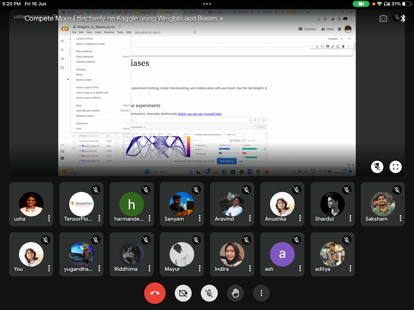
Compete More Effectively on Kaggle using Weights and Biases by TFUG Hajipur was a meetup to explore techniques using Weights and Biases to improve model performance in Kaggle competitions. Usha Rengaraju (India) joined as a speaker and delivered her insights on Kaggle and strategies to win competitions. She shared tips and tricks and demonstrated how to set up a W&B account and how to integrate with Google Colab and Kaggle.

Skeleton Based Action Recognition: A failed attempt by ML GDE Ayush Thakur (India) is a discussion post about documenting his learnings from competing in the Kaggle competition, Google - Isolated Sign Language Recognition. He shared his repository, training logs, and ideas he approached in the competition. Plus, his article Keras Dense Layer: How to Use It Correctly) explored what the dense layer in Keras is and how it works in practice.

On-device ML

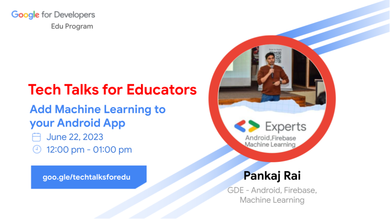
Add Machine Learning to your Android App by ML GDE Pankaj Rai (India) at Tech Talks for Educators was a session on on-device ML and how to add ML capabilities to Android apps such as object detection and gesture detection. He explained capabilities of ML Kit, MediaPipe, TF Lite and how to use these tools. 700+ people registered for his talk.

In MediaPipe with a bit of Bard at I/O Extended Singapore 2023, ML GDE Martin Andrews (Singapore) shared how MediaPipe fits into the ecosystem, and showed 4 different demonstrations of MediaPipe functionality: audio classification, facial landmarks, interactive segmentation, and text classification.

Adding ML to our apps with Google ML Kit and MediaPipe by ML GDE Juan Guillermo Gomez Torres (Bolivia) introduced ML Kit & MediaPipe, and the benefits of on-device ML. In Startup Academy México (Google for Startups), he shared how to increase the value for clients with ML and MediaPipe.

LLM

Introduction to Google's PaLM 2 API by ML GDE Hannes Hapke (United States) introduced how to use PaLM2 and summarized major advantages of it. His another article The role of ML Engineering in the time of GPT-4 & PaLM 2 explains the role of ML experts in finding the right balance and alignment among stakeholders to optimally navigate the opportunities and challenges posed by this emerging technology. He did presentations under the same title at North America Connect 2023 and the GDG Portland event.

Image of a cellphone with ChatBard on the display in front of a computer display with Firebase PaLM in Cloud Firestore

ChatBard : An Intelligent Customer Service Center App by ML GDE Ruqiya Bin Safi (Saudi Arabia) is an intelligent customer service center app powered by generative AI and LLMs using PaLM2 APIs.

Bard can now code and put that code in Colab for you by ML GDE Sam Witteveen (Singapore) showed how Bard makes code. He runs a Youtube channel exploring ML and AI, with playlists such as Generative AI, Paper Reviews, LLMs, and LangChain.

Google’s Bard Can Write Code by ML GDE Bhavesh Bhatt (India) shows the coding capabilities of Bard, how to create a 2048 game with it, and how to add some basic features to the game. He also uploaded videos about LangChain in a playlist and introduced Google Cloud’s new course on Generative AI in this video.

Screengrab of GDG Deep Learning Course Attention Mechanisms and Transformers led by Ruqiya Bin Safi ML GDE & WTM Ambassador, @Ru0Sa

Attention Mechanisms and Transformers by GDG Cloud Saudi talked about Attention and Transformer in NLP and ML GDE Ruqiya Bin Safi (Saudi Arabia) participated as a speaker. Another event, Hands-on with the PaLM2 API to create smart apps(Jeddah) explored what LLMs, PaLM2, and Bard are, how to use PaLM2 API, and how to create smart apps using PaLM2 API.

Hands-on with Generative AI: Google I/O Extended [Virtual] by ML GDE Henry Ruiz (United States) and Web GDE Rabimba Karanjai (United States) was a workshop on generative AI showing hands-on demons of how to get started using tools such as PaLM API, Hugging Face Transformers, and LangChain framework.

Generative AI with Google PaLM and MakerSuite by ML GDE Kuan Hoong (Malaysia) at Google I/O Extended George Town 2023 was a talk about LLMs with Google PaLM and MakerSuite. The event hosted by GDG George Town and also included ML topics such as LLMs, responsible AI, and MLOps.

Intor to Gen AI with PaLM API and MakerSuite led by GUS Luis Gustavo and Tensorflow User Group Sao Paolo

Intro to Gen AI with PaLM API and MakerSuite by TFUG São Paulo was for people who want to learn generative AI and how Google tools can help with adoption and value creation. They covered how to start prototyping Gen AI ideas with MakerSuite and how to access advanced features of PaLM2 and PaLM API. The group also hosted Opening Pandora's box: Understanding the paper that revolutionized the field of NLP (video) and ML GDE Pedro Gengo (Brazil) and ML GDE Vinicius Caridá (Brazil) shared the secret behind the famous LLM and other Gen AI models.The group members studied Attention Is All You Need paper together and learned the full potential that the technology can offer.

Language models which PaLM can speak, see, move, and understand by GDG Cloud Taipei was for those who want to understand the concept and application of PaLM. ML GED Jerry Wu (Taiwan) shared the PaLM’s main characteristics, functions, and etc.

Flow chart illustrating flexible serving structure of stable diffusion

Serving With TF and GKE: Stable Diffusion by ML GDE Chansung Park (Korea) and ML GDE Sayak Paul (India) discusses how TF Serving and Kubernetes Engine can serve a system with online deployment. They broke down Stable Diffusion into main components and how they influence the subsequent consideration for deployment. Then they also covered the deployment-specific bits such as TF Serving deployment and k8s cluster configuration.

TFX + W&B Integration by ML GDE Chansung Park (Korea) shows how KerasTuner can be used with W&B’s experiment tracking feature within the TFX Tuner component. He developed a custom TFX component to push a full-trained model to the W&B Artifact store and publish a working application on Hugging Face Space with the current version of the model. Also, his talk titled, ML Infra and High Level Framework in Google Cloud Platform, delivered what MLOps is, why it is hard, why cloud + TFX is a good starter, and how TFX is seamlessly integrated with Vertex AI and Dataflow. He shared use cases from the past projects that he and ML GDE Sayak Paul (India) have done in the last 2 years.

Open and Collaborative MLOps by ML GDE Sayak Paul (India) was a talk about why openness and collaboration are two important aspects of MLOps. He gave an overview of Hugging Face Hub and how it integrates well with TFX to promote openness and collaboration in MLOps workflows.

ML Research

Paper review: PaLM 2 Technical Report by ML GDE Grigory Sapunov (UK) looked into the details of PaLM2 and the paper. He shares reviews of papers related to Google and DeepMind through his social channels and here are some of them: Model evaluation for extreme risks (paper), Faster sorting algorithms discovered using deep reinforcement learning (paper), Power-seeking can be probable and predictive for trained agents (paper).

Learning JAX in 2023: Part 3 — A Step-by-Step Guide to Training Your First Machine Learning Model with JAX by ML GDE Aritra Roy Gosthipaty (India) and ML GDE Ritwik Raha (India) shows how JAX can train linear and nonlinear regression models and the usage of PyTrees library to train a multilayer perceptron model. In addition, at May 2023 Meetup hosted by TFUG Mumbai, they gave a talk titled Decoding End to End Object Detection with Transformers and covered the architecture of the mode and the various components that led to DETR’s inception.

20 steps to train a deployed version of the GPT model on TPU by ML GDE Jerry Wu (Taiwan) shared how to use JAX and TPU to train and infer Chinese question-answering data.

Photo of the audience from the back of the room at Developer Space @Google Singapore during Multimodal Transformers - Custom LLMs, ViTs & BLIPs

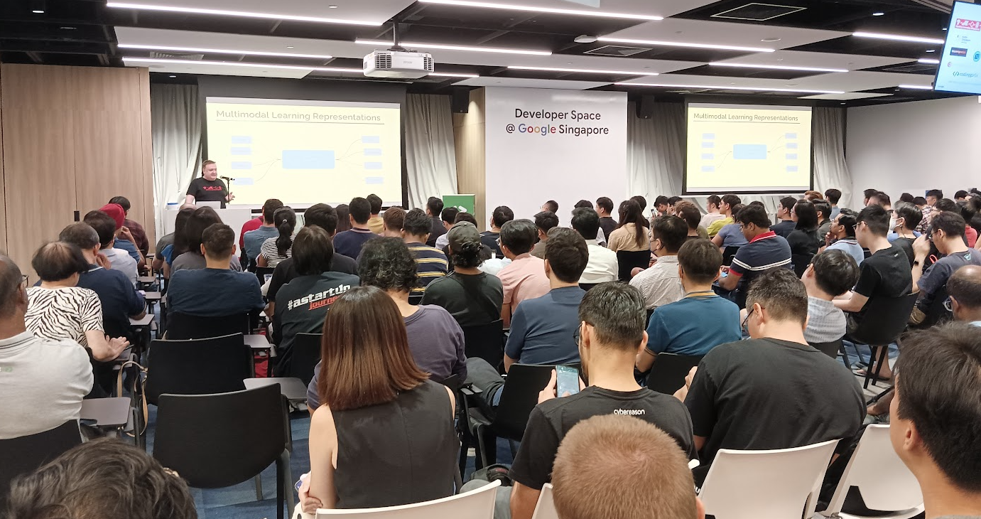
Multimodal Transformers - Custom LLMs, ViTs & BLIPs by TFUG Singapore looked at what models, systems, and techniques have come out recently related to multimodal tasks. ML GDE Sam Witteveen (Singapore) looked into various multimodal models and systems and how you can build your own with the PaLM2 Model. In June, this group invited Blaise Agüera y Arcas (VP and Fellow at Google Research) and shared the Cerebra project and the research going on at Google DeepMind including the current and future developments in generative AI and emerging trends.

TensorFlow

Training a recommendation model with dynamic embeddings by ML GDE Thushan Ganegedara (Australia) explains how to build a movie recommender model by leveraging TensorFlow Recommenders (TFRS) and TensorFlow Recommenders Addons (TFRA). The primary focus was to show how the dynamic embeddings provided in the TFRA library can be used to dynamically grow and shrink the size of the embedding tables in the recommendation setting.

Screengrab of a tweet by Mathis Hammel showcasing his talk, 'How I built the most efficient deepfake detector in the world for $100'

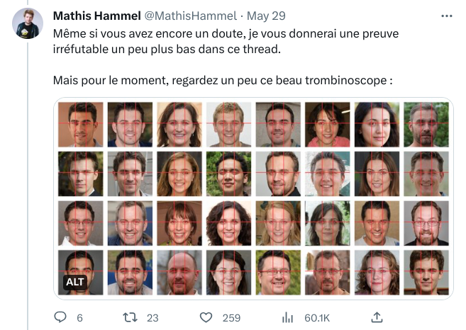
How I built the most efficient deepfake detector in the world for $100 by ML GDE Mathis Hammel (France) was a talk exploring a method to detect images generated via ThisPersonDoesNotExist.com and even a way to know the exact time the photo was produced. Plus, his Twitter thread, OSINT Investigation on LinkedIn, investigated a network of fake companies on LinkedIn. He used a homemade tool based on a TensorFlow model and hosted it on Google Cloud. Technical explanations of generative neural networks were also included. More than 701K people viewed this thread and it got 1200+ RTs and 3100+ Likes.

Screengrab of Few-shot learning: Creating a real-time object detection using TensorFlow and python by ML GDE Hugo Zanini

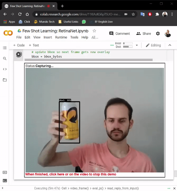
Few-shot learning: Creating a real-time object detection using TensorFlow and Python by ML GDE Hugo Zanini (Brazil) shows how to take pictures of an object using a webcam, label the images, and train a few-shot learning model to run in real-time. Also, his article, Custom YOLOv7 Object Detection with TensorFlow.js explains how he trained a custom YOLOv7 model to run it directly in the browser in real time and offline with TensorFlow.js.

The Lord of the Words Transformation of a Sequence Encoder/Decoder Attention

The Lord of the Words : The Return of the experiments with DVC (slides) by ML GDE Gema Parreno Piqueras (Spain) was a talk explaining Transformers in the neural machine learning scenario, and how to use Tensorflow and DVC. In the project, she used Tensorflow Datasets translation catalog to load data from various languages, and TensorFlow Transformers library to train several models.

Accelerate your TensorFlow models with XLA (slides) and Ship faster TensorFlow models with XLA by ML GDE Sayak Paul (India) shared how to accelerate TensorFlow models with XLA in Cloud Community Days Kolkata 2023 and Cloud Community Days Pune 2023.

Setup of NVIDIA Merlin and Tensorflow for Recommendation Models by ML GDE Rubens Zimbres (Brazil) presented a review of recommendation algorithms as well as the Two Towers algorithm, and setup of NVIDIA Merlin on premises and on Vertex AI.

Cloud

AutoML pipeline for tabular data on VertexAI in Go by ML GDE Paolo Galeone (Italy) delved into the development and deployment of tabular models using VertexAI and AutoML with Go, showcasing the actual Go code and sharing insights gained through trial & error and extensive Google research to overcome documentation limitations.

Beyond images: searching information in videos using AI (slides) by ML GDE Pedro Gengo (Brazil) and ML GDE Vinicius Caridá (Brazil) showed how to create a search engine where you can search for information in videos. They presented an architecture where they transcribe the audio and caption the frames, convert this text into embeddings, and save them in a vector DB to be able to search given a user query.

The secret sauce to creating amazing ML experiences for developers by ML GDE Gant Laborde (United States) was a podcast sharing his “aha” moment, 20 years of experience in ML, and the secret to creating enjoyable and meaningful experiences for developers.

What's inside Google’s Generative AI Studio? by ML GDE Gad Benram (Portugal) shared the preview of the new features and what you can expect from it. Additionally, in How to pitch Vertex AI in 2023, he shared the six simple and honest sales pitch points for Google Cloud representatives on how to convince customers that Vertex AI is the right platform.

In How to build a conversational AI Augmented Reality Experience with Sachin Kumar, ML GDE Sachin Kumar (Qatar) talked about how to build an AR app combining multiple technologies like Google Cloud AI, Unity, and etc. The session walked through the step-by-step process of building the app from scratch.

Machine Learning on Google Cloud Platform led by Nitin Tiwari, Google Developer Expert - Machine Learning, Software Engineer @LTMIMindtree

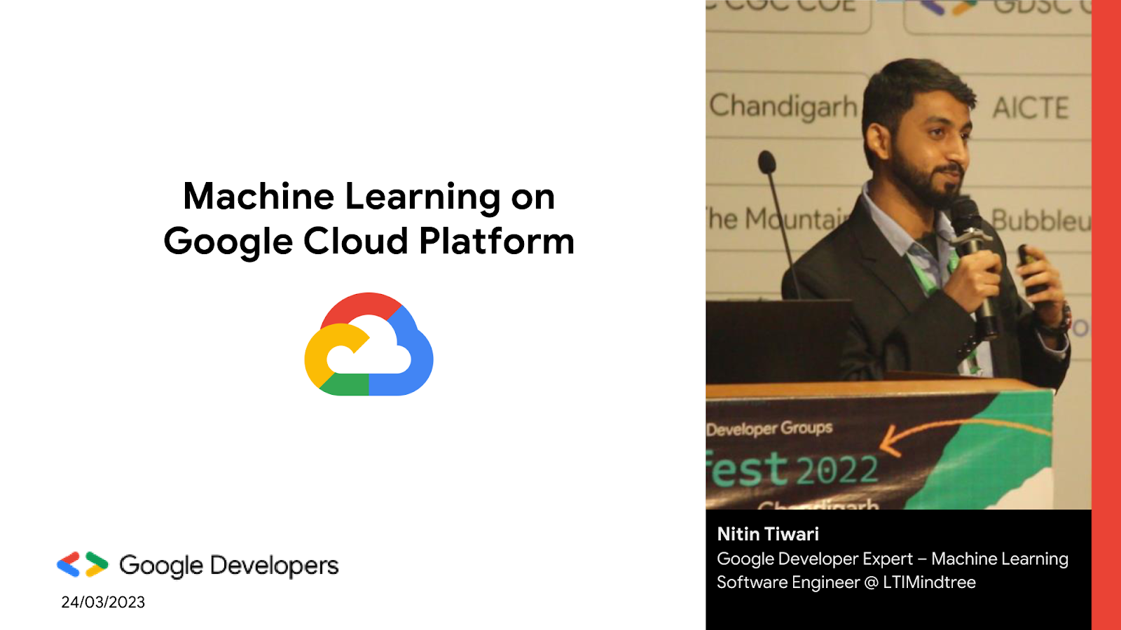
Machine Learning on Google Cloud Platform by ML GDE Nitin Tiwari (India) was a mentoring aiming to provide students with an in-depth understanding of the processes involved in training an ML model and deploying it using GCP. In Building robust ML solutions with TensorFlow and GCP, he shared how to leverage the capabilities of GCP and TensorFlow for ML solutions and deploy custom ML models.

Data to AI on Google cloud: Auto ML, Gen AI, and more by TFUG Prayagraj educated students on how to leverage Google Cloud’s advanced AI technologies, including AutoML and generative AI.

Source: Google for Developers Blog - News about Web, Mobile, AI and Cloud

Kubeflow joins the CNCF family

We are thrilled to announce a major milestone in the journey of the Kubeflow project. After a comprehensive review process and several months of meticulous preparation, Kubeflow has been accepted by the Cloud Native Computing Foundation (CNCF) as an incubating project. This momentous step marks a new chapter in our collaborative and open approach to accelerating machine learning (ML) in the cloud native ecosystem.

The acceptance of Kubeflow into the incubation stage by the CNCF reflects not just the project's maturity, but also its widespread adoption and expanding user base. It underscores the tremendous value of the diverse suite of components that Kubeflow provides, including Notebooks, Pipelines, Training Operators, Katib, Central Dashboard, Manifests, and many more. These tools have been instrumental in creating a cohesive, end-to-end ML platform that streamlines the development and deployment of ML workflows.

Furthermore, the alignment of Kubeflow with the CNCF acknowledges the project's foundational reliance on several existing CNCF projects such as Argo, Cert-Manager, and Istio. The joining of Kubeflow with the CNCF will serve to strengthen these existing relationships and foster greater collaboration among cloud native projects, leading to even more robust and innovative solutions for users.

Looking ahead, Google and the Kubeflow community are eager to collaborate with the CNCF on the transition process. Rest assured, our commitment to Kubeflow's ongoing development remains unwavering during this transition. We will continue to support new feature development, plan and execute upcoming releases, and strive to deliver further improvements to the Kubeflow project.

We extend our heartfelt thanks to the CNCF Technical Oversight Committee and the wider CNCF community for their support and recognition of the Kubeflow project. We look forward to this exciting new phase in our shared journey towards advancing machine learning in the cloud native landscape.

As Kubeflow continues to evolve, we invite developers, data scientists, ML engineers, and all other interested individuals to join us in shaping the future of cloud native machine learning. Let's innovate together, with Kubeflow and the CNCF, to make machine learning workflows more accessible, manageable, and scalable than ever before!

By James Liu – GCP Cloud AI

The benefits of IRL

Receding Horizon Inverse Planning

Routing wins

Conclusion

Acknowledgements

Source: Google AI Blog

Large-scale scientific computation with accelerators

Framework validation and homogeneous isotropic turbulence

A new era for turbulent flows research

Acknowledgements

Source: Google AI Blog

TSMixer architecture

Evaluation on long-term forecasting benchmarks

Ablation study

Evaluation on M5: Effectiveness of cross-variate information

Conclusion

Acknowledgements

Source: Google AI Blog

SayTap method

Results

Following simple and direct commands

Following unstructured or vague commands

Conclusion and future work

Acknowledgements

Source: Google AI Blog

Reward Translator: Translating user instructions to reward functions

Motion Descriptor

Reward Coder

Motion Controller: Translating reward functions to robot actions

Examples

Robot dog

Dexterous manipulator

Validation on real robots

Conclusion

Acknowledgements

Source: Google AI Blog

Comparison to previous work

Informing LLM decision making with a user study

General framework

Results

Conclusion

Acknowledgements

Source: Google AI Blog

Overview of contributions

A computation-friendly pruning formulation

Scalable optimization algorithms

Experiments

Conclusion, limitations, and future work

Acknowledgements

Source: Google AI Blog

What tech area has you most fascinated right now, and why?

How do you like to learn new services, tools, and applications?

What are some exciting projects you have in flight right now?

What engages you outside of the technology world?

What brought you into the Innovators program?

What's one thing our readers should do next?

Source: Google for Developers Blog - News about Web, Mobile, AI and Cloud

ML Training Campaigns Summary

Community Highlights

Keras

Kaggle

On-device ML

LLM

ML Research

TensorFlow

Cloud

Source: Google for Developers Blog - News about Web, Mobile, AI and Cloud

Source: Google Open Source Blog