Tag Archives: machine learning

A New Lens on Understanding Generalization in Deep Learning

Understanding generalization is one of the fundamental unsolved problems in deep learning. Why does optimizing a model on a finite set of training data lead to good performance on a held-out test set? This problem has been studied extensively in machine learning, with a rich history going back more than 50 years. There are now many mathematical tools that help researchers understand generalization in certain models. Unfortunately, most of these existing theories fail when applied to modern deep networks — they are both vacuous and non-predictive in realistic settings. This gap between theory and practice is largest for overparameterized models, which in theory have the capacity to overfit their train sets, but often do not in practice.

In “The Deep Bootstrap Framework: Good Online Learners are Good Offline Generalizers”, accepted at ICLR 2021, we present a new framework for approaching this problem by connecting generalization to the field of online optimization. In a typical setting, a model trains on a finite set of samples, which are reused for multiple epochs. But in online optimization, the model has access to an infinite stream of samples, and can be iteratively updated while processing this stream. In this work, we find that models that train quickly on infinite data are the same models that generalize well if they are instead trained on finite data. This connection brings new perspectives on design choices in practice, and lays a roadmap for understanding generalization from a theoretical perspective.

The Deep Bootstrap Framework
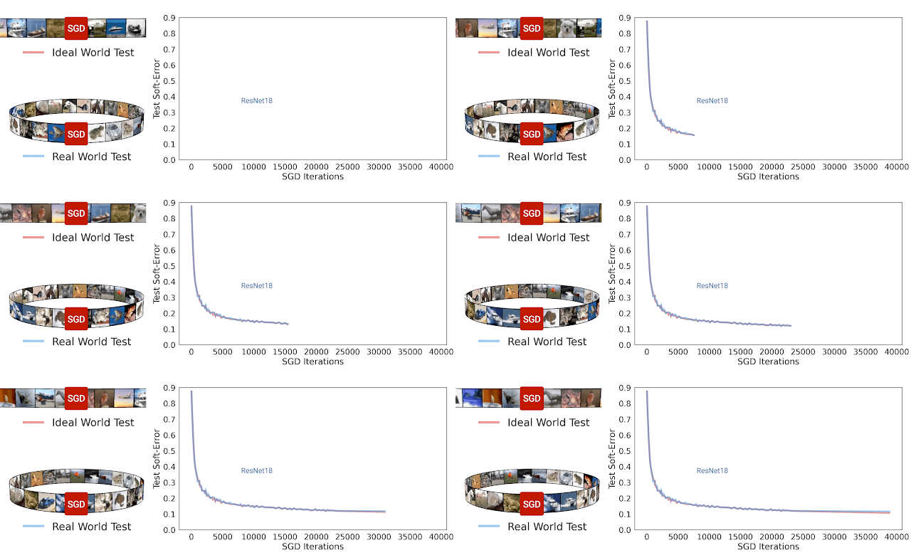
The main idea of the Deep Bootstrap framework is to compare the real world, where there is finite training data, to an "ideal world", where there is infinite data. We define these as:

  • Real World (N, T): Train a model on N train samples from a distribution, for T minibatch stochastic gradient descent (SGD) steps, re-using the same N samples in multiple epochs, as usual. This corresponds to running SGD on the empirical loss (loss on training data), and is the standard training procedure in supervised learning.
  • Ideal World (T): Train the same model for T steps, but use fresh samples from the distribution in each SGD step. That is, we run the exact same training code (same optimizer, learning-rates, batch-size, etc.), but sample a fresh train set in each epoch instead of reusing samples. In this ideal world setting, with an effectively infinite "train set", there is no difference between train error and test error.
Test soft-error for ideal world and real world during SGD iterations for ResNet-18 architecture. We see that the two errors are similar.

A priori, one might expect the real and ideal worlds may have nothing to do with each other, since in the real world the model sees a finite number of examples from the distribution while in the ideal world the model sees the whole distribution. But in practice, we found that the real and ideal models actually have similar test error.

In order to quantify this observation, we simulated an ideal world setting by creating a new dataset, which we call CIFAR-5m. We trained a generative model on CIFAR-10, which we then used to generate ~6 million images. The scale of the dataset was chosen to ensure that it is “virtually infinite” from the model’s perspective, so that the model never resamples the same data. That is, in the ideal world, the model sees an entirely fresh set of samples.

Samples from CIFAR-5m

The figure below presents the test error of several models, comparing their performance when trained on CIFAR-5m data in the real world setting (i.e., re-used data) and the ideal world (“fresh” data). The solid blue line shows a ResNet model in the real world, trained on 50K samples for 100 epochs with standard CIFAR-10 hyperparameters. The dashed blue line shows the corresponding model in the ideal world, trained on 5 million samples in a single pass. Surprisingly, these worlds have very similar test error — the model in some sense "doesn't care" whether it sees re-used samples or fresh ones.

The real world model is trained on 50K samples for 100 epochs, and the ideal world model is trained on 5M samples for a single epoch. The lines show the test error vs. the number of SGD steps.

This also holds for other architectures, e.g., a Multi-Layer-Perceptron (red), a Vision Transformer (green), and across many other settings of architecture, optimizer, data distribution, and sample size. These experiments suggest a new perspective on generalization: models that optimize quickly (on infinite data), generalize well (on finite data). For example, the ResNet model generalizes better than the MLP model on finite data, but this is "because" it optimizes faster even on infinite data.

Understanding Generalization from Optimization Behavior
The key observation is that real world and ideal world models remain close, in test error, for all timesteps, until the real world converges (< 1% train error). Thus, one can study models in the real world by studying their corresponding behavior in the ideal world.

This means that the generalization of the model can be understood in terms of its optimization performance under two frameworks:

  1. Online Optimization: How fast the ideal world test error decreases
  2. Offline Optimization: How fast the real world train error converges

Thus, to study generalization, we can equivalently study the two terms above, which can be conceptually simpler, since they only involve optimization concerns. Based on this observation, good models and training procedures are those that (1) optimize quickly in the ideal world and (2) do not optimize too quickly in the real world.

All design choices in deep learning can be viewed through their effect on these two terms. For example, some advances like convolutions, skip-connections, and pre-training help primarily by accelerating ideal world optimization, while other advances like regularization and data-augmentation help primarily by decelerating real world optimization.

Applying the Deep Bootstrap Framework
Researchers can use the Deep Bootstrap framework to study and guide design choices in deep learning. The principle is: whenever one makes a change that affects generalization in the real world (the architecture, learning-rate, etc.), one should consider its effect on (1) the ideal world optimization of test error (faster is better) and (2) the real world optimization of train error (slower is better).

For example, pre-training is often used in practice to help generalization of models in small-data regimes. However, the reason that pre-training helps remains poorly understood. One can study this using the Deep Bootstrap framework by looking at the effect of pre-training on terms (1) and (2) above. We find that the primary effect of pre-training is to improve the ideal world optimization (1) — pre-training turns the network into a "fast learner" for online optimization. The improved generalization of pretrained models is thus almost exactly captured by their improved optimization in the ideal world. The figure below shows this for Vision-Transformers (ViT) trained on CIFAR-10, comparing training from scratch vs. pre-training on ImageNet.

Effect of pre-training — pre-trained ViTs optimize faster in the ideal world.

One can also study data-augmentation using this framework. Data-augmentation in the ideal world corresponds to augmenting each fresh sample once, as opposed to augmenting the same sample multiple times. This framework implies that good data-augmentations are those that (1) do not significantly harm ideal world optimization (i.e., augmented samples don't look too "out of distribution") or (2) inhibit real world optimization speed (so the real world takes longer to fit its train set).

The main benefit of data-augmentation is through the second term, prolonging the real world optimization time. As for the first term, some aggressive data augmentations (mixup/cutout) can actually harm the ideal world, but this effect is dwarfed by the second term.

Concluding Thoughts
The Deep Bootstrap framework provides a new lens on generalization and empirical phenomena in deep learning. We are excited to see it applied to understand other aspects of deep learning in the future. It is especially interesting that generalization can be characterized via purely optimization considerations, which is in contrast to many prevailing approaches in theory. Crucially, we consider both online and offline optimization, which are individually insufficient, but that together determine generalization.

The Deep Bootstrap framework can also shed light on why deep learning is fairly robust to many design choices: many kinds of architectures, loss functions, optimizers, normalizations, and activation functions can generalize well. This framework suggests a unifying principle: that essentially any choice that works well in the online optimization setting will also generalize well in the offline setting.

Finally, modern neural networks can be either overparameterized (e.g., large networks trained on small data tasks) or underparmeterized (e.g., OpenAI's GPT-3, Google's T5, or Facebook's ResNeXt WSL). The Deep Bootstrap framework implies that online optimization is a crucial factor to success in both regimes.

Acknowledgements
We are thankful to our co-author, Behnam Neyshabur, for his great contributions to the paper and valuable feedback on the blog. We thank Boaz Barak, Chenyang Yuan, and Chiyuan Zhang for helpful comments on the blog and paper.

Source: Google AI Blog


ML Kit is now in GA & Introducing Selfie Segmentation

Posted by Kenny Sulaimon, Product Manager, ML Kit Chengji Yan, Suril Shah, Buck Bourdon, Software Engineers, ML Kit, Shiyu Hu, Technical Lead, ML Kit Dong Chen, Technical Lead, ML Kit

At the end of 2020, we introduced the Entity Extraction API to our ML Kit SDK, making it even easier to detect and perform actions on text within mobile apps. Since then, we’ve been hard at work updating our existing APIs with new functionality and also fine tuning Selfie Segmentation with the help of our partners in the ML Kit early access program.

Today we are excited to officially add Selfie Segmentation to the ML Kit lineup, introduce a few enhancements we’ve made to our popular Pose Detection API and announce that ML Kit has graduated to general availability!

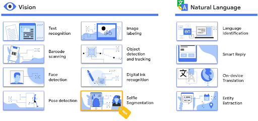
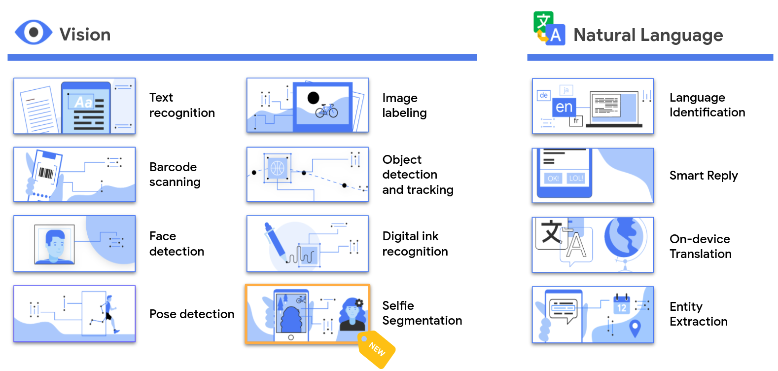
Natural language graphic

General Availability

ML Kit image

(ML Kit is now in General Availability)

We launched ML Kit back in 2018 in order to make it easy for developers on Android and iOS to use machine learning within their apps. Over the last two years we have rapidly expanded our set of APIs to help with both vision and natural language processing based use cases.

Thanks to the overwhelmingly positive response, developer feedback and a ton of adoption across both Android and iOS, we are ready to drop the beta label and officially announce the general availability of ML Kit’s APIs. All of our APIs (except Selfie Segmentation, Pose Detection, and Entity Extraction) are now in general availability!

Selfie Segmentation

Selfie Segmentation photo

(Example of ML Kit Selfie Segmentation)

With the increased usage of selfie cameras and webcams in today's world, being able to quickly and easily add effects to camera experiences has become a necessity for many app developers.

ML Kit's Selfie Segmentation API allows developers to easily separate the background from users within a scene and focus on what matters. Adding cool effects to selfies or inserting your users into interesting background environments has never been easier. The model works on live and still images, and both half and full body subjects.

Under The Hood

Under the hood graph

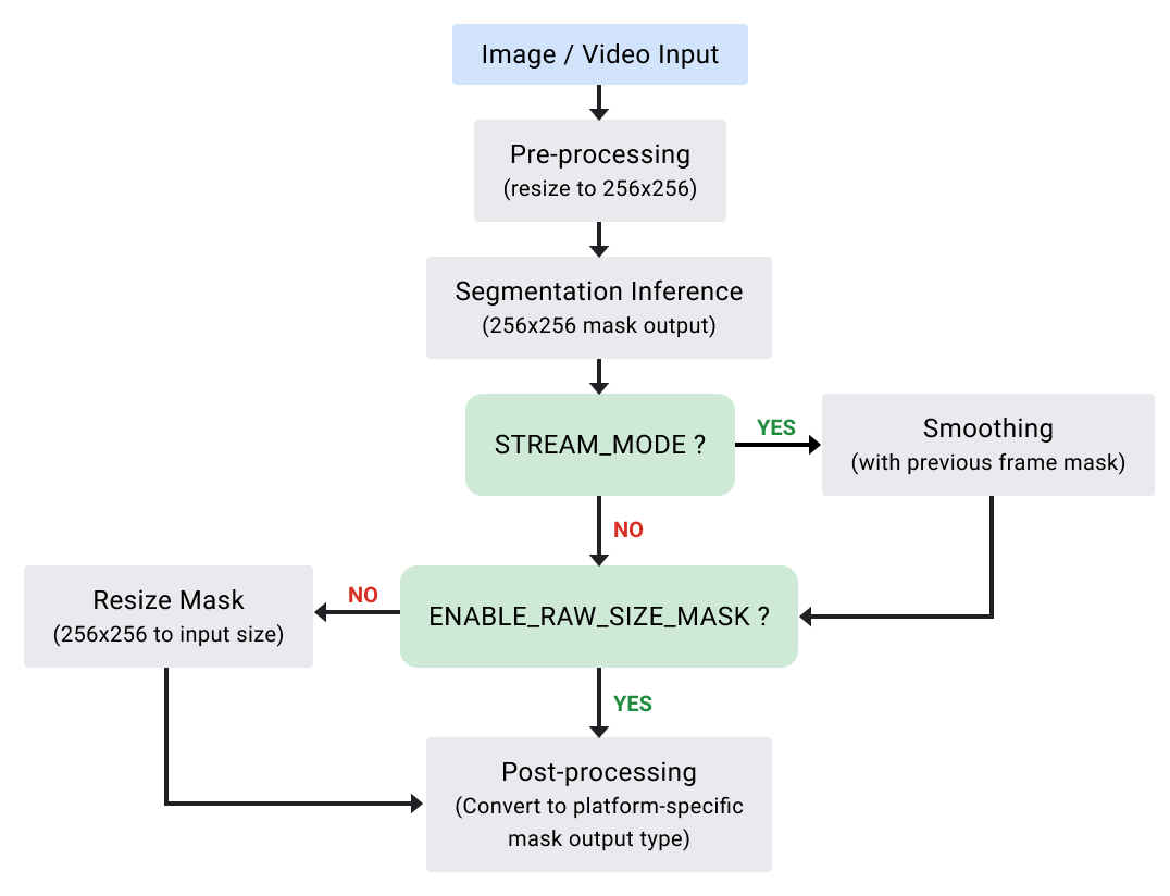
(Diagram of Selfie Segmentation API)

The Selfie Segmentation API takes an input image and produces an output mask. Each pixel of the mask is assigned a float number that has a range between [0.0, 1.0]. The closer the number is to 1.0, the higher the confidence that the pixel represents a person, and vice versa.

The API works with static images and live video use cases. During live video (stream_mode), the API will leverage output from previous frames to return smoother segmentation results.

We’ve also implemented a “RAW_SIZE_MASK” option to give developers more options for mask output. By default, the mask produced will be the same size as the input image. If the RAW_SIZE_MASK option is enabled, then the mask will be the size of the model output (256x256). This option makes it easier to apply customized rescaling logic or reduces latency if rescaling to the input image size is not needed for your use case.

Pose Detection Update

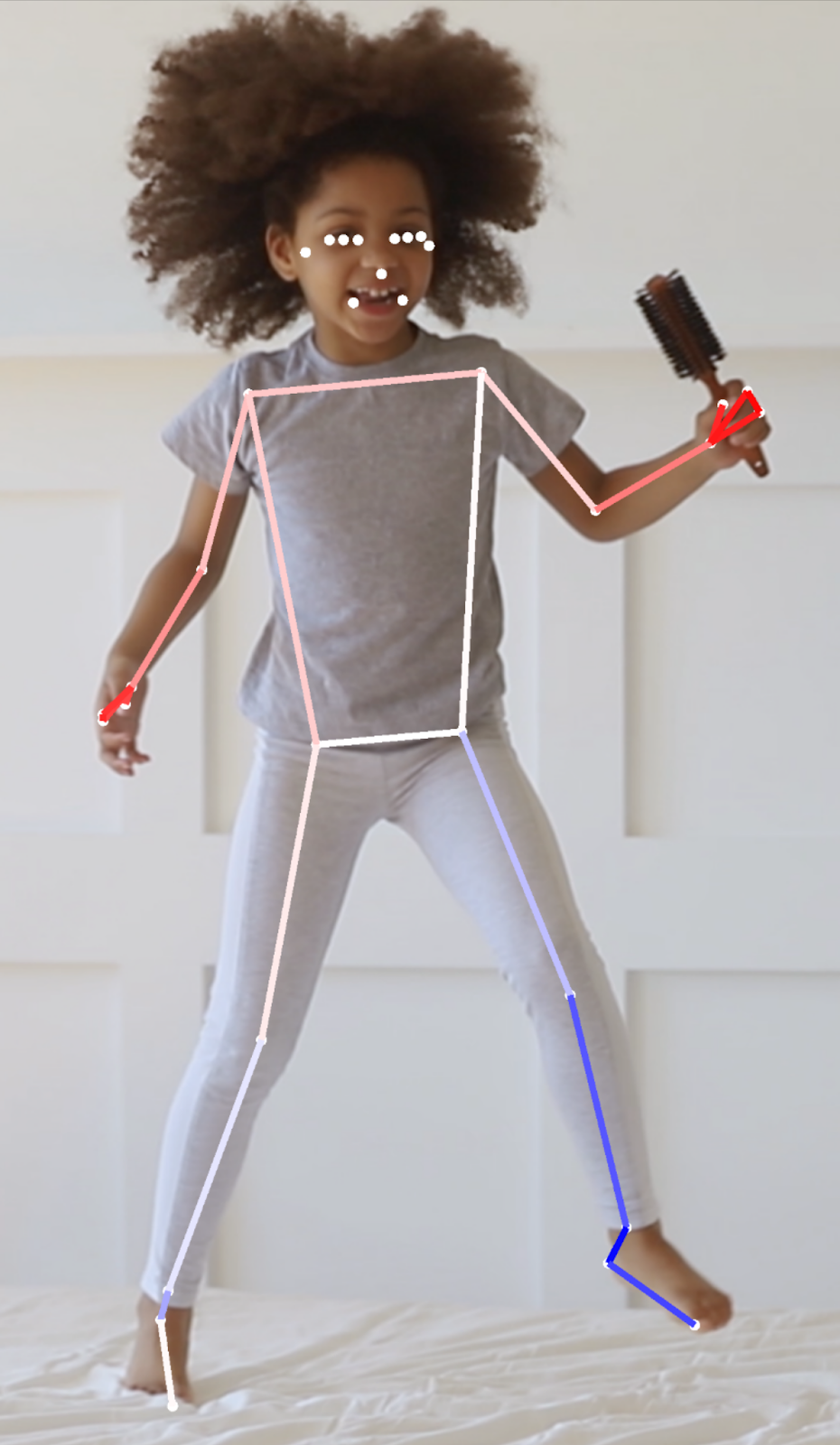
Example of Pose Detection API

(Example of updated Pose Detection API; colors represent the Z value)

Last month, we updated our state-of-the-art Pose Detection API with a new model and new features. A quick summary of the enhancements is listed below:

  • More poses added The API now recognizes more poses, targeting fitness and yoga use cases, especially when a user is directly facing the camera.
  • 50% size reduction The base and accurate pose models are now significantly smaller. This change does not impact the quality of the models.
  • Z Coordinate for depth analysis The API now outputs a depth coordinate Z to help determine whether parts of the user's body are in front or behind the user’s hips.

Z Coordinate

The Z Coordinate is an experimental feature that is calculated for every point (excluding the face). The estimate is provided using synthetic data, obtained via the GHUM model (articulated 3D human shape model).

It is measured in "image pixels" like the X and Y coordinates. The Z axis is perpendicular to the camera and passes between a subject's hips. The origin of the Z axis is approximately the center point between the hips (left/right and front/back relative to the camera). Negative Z values are towards the camera; positive values are away from it. The Z coordinate does not have an upper or lower bound.

For more information on the Pose Detection changes, please see our API documentation.

Pose Classification

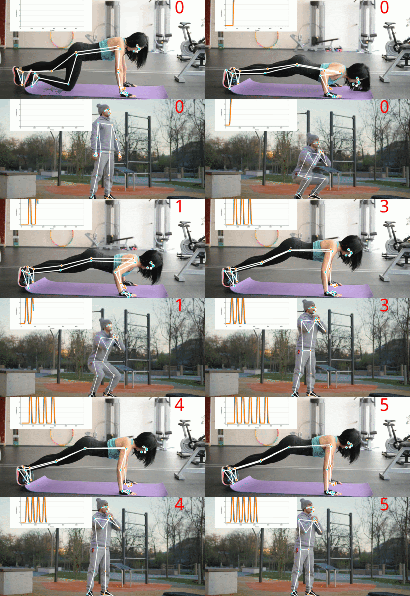
After the release of Pose Detection, we’ve received quite a bit of requests from developers to help with classifying specific poses within their apps. To help tackle this problem, we partnered with the MediaPipe team to release a pose classification tutorial and Google Colab. In the classification tutorial, we demonstrate how to build and run a custom pose classifier within the ML Kit Android sample app and also demo a simple push-up and squat rep counter using the classifier.

Example of Pose classification and repetition counting with MLKit Pose

(Example of Pose classification and repetition counting with MLKit Pose)

For a deep dive into building your own pose classifier with different camera angles, environment conditions, body shapes etc, please see the pose classification tutorial.

For more general classification tips, please see our Pose Classification Options page on the ML Kit website.

Beyond General Availability

It has been an exciting two years getting ML Kit to general availability and we couldn’t have gotten here without your help and feedback. As we continue to introduce new APIs such as Selfie Segmentation and Pose Detection, your feedback is more important than ever. Please continue to share your enhancement requests and questions with our development team or reach out through our community channels. Let’s build a smarter future together.

Accelerating Neural Networks on Mobile and Web with Sparse Inference

On-device inference of neural networks enables a variety of real-time applications, like pose estimation and background blur, in a low-latency and privacy-conscious way. Using ML inference frameworks like TensorFlow Lite with XNNPACK ML acceleration library, engineers optimize their models to run on a variety of devices by finding a sweet spot between model size, inference speed and the quality of the predictions.

One way to optimize a model is through use of sparse neural networks [1, 2, 3], which have a significant fraction of their weights set to zero. In general, this is a desirable quality as it not only reduces the model size via compression, but also makes it possible to skip a significant fraction of multiply-add operations, thereby speeding up inference. Further, it is possible to increase the number of parameters in a model and then sparsify it to match the quality of the original model, while still benefiting from the accelerated inference. However, the use of this technique remains limited in production largely due to a lack of tools to sparsify popular convolutional architectures as well as insufficient support for running these operations on-device.

Today we announce the release of a set of new features for the XNNPACK acceleration library and TensorFlow Lite that enable efficient inference of sparse networks, along with guidelines on how to sparsify neural networks, with the goal of helping researchers develop their own sparse on-device models. Developed in collaboration with DeepMind, these tools power a new generation of live perception experiences, including hand tracking in MediaPipe and background features in Google Meet, accelerating inference speed from 1.2 to 2.4 times, while reducing the model size by half. In this post, we provide a technical overview of sparse neural networks — from inducing sparsity during training to on-device deployment — and offer some ideas on how researchers might create their own sparse models.

Comparison of the processing time for the dense (left) and sparse (right) models of the same quality for Google Meet background features. For readability, the processing time shown is the moving average across 100 frames.

Sparsifying a Neural Network
Many modern deep learning architectures, like MobileNet and EfficientNetLite, are primarily composed of depthwise convolutions with a small spatial kernel and 1x1 convolutions that linearly combine features from the input image. While such architectures have a number of potential targets for sparsification, including the full 2D convolutions that frequently occur at the beginning of many networks or the depthwise convolutions, it is the 1x1 convolutions that are the most expensive operators as measured by inference time. Because they account for over 65% of the total compute, they are an optimal target for sparsification.

Architecture Inference Time
MobileNet 85%
MobileNetV2 71%
MobileNetV3 71%
EfficientNet-Lite   66%
Comparison of inference time dedicated to 1x1 convolutions in % for modern mobile architectures.

In modern on-device inference engines, like XNNPACK, the implementation of 1x1 convolutions as well as other operations in the deep learning models rely on the HWC tensor layout, in which the tensor dimensions correspond to the height, width, and channel (e.g., red, green or blue) of the input image. This tensor configuration allows the inference engine to process the channels corresponding to each spatial location (i.e., each pixel of an image) in parallel. However, this ordering of the tensor is not a good fit for sparse inference because it sets the channel as the innermost dimension of the tensor and makes it more computationally expensive to access.

Our updates to XNNPACK enable it to detect if a model is sparse. If so, it switches from its standard dense inference mode to sparse inference mode, in which it employs a CHW (channel, height, width) tensor layout. This reordering of the tensor allows for an accelerated implementation of the sparse 1x1 convolution kernel for two reasons: 1) entire spatial slices of the tensor can be skipped when the corresponding channel weight is zero following a single condition check, instead of a per-pixel test; and 2) when the channel weight is non-zero, the computation can be made more efficient by loading neighbouring pixels into the same memory unit. This enables us to process multiple pixels simultaneously, while also performing each operation in parallel across several threads. Together these changes result in a speed-up of 1.8x to 2.3x when at least 80% of the weights are zero.

In order to avoid converting back and forth between the CHW tensor layout that is optimal for sparse inference and the standard HWC tensor layout after each operation, XNNPACK provides efficient implementations of several CNN operators in CHW layout.

Guidelines for Training Sparse Neural Networks
To create a sparse neural network, the guidelines included in this release suggest one start with a dense version and then gradually set a fraction of its weights to zero during training. This process is called pruning. Of the many available techniques for pruning, we recommend using magnitude pruning (available in the TF Model Optimization Toolkit) or the recently introduced RigL method. With a modest increase in training time, both of these can successfully sparsify deep learning models without degrading their quality. The resulting sparse models can be stored efficiently in a compressed format that reduces the size by a factor of two compared to their dense equivalent.

The quality of sparse networks is influenced by several hyperparameters, including training time, learning rate and schedules for pruning. The TF Pruning API provides an excellent example of how to select these, as well as some tips for training such models. We recommend running hyperparameter searches to find the sweet spot for your application.

Applications
We demonstrate that it is possible to sparsify classification tasks, dense segmentation (e.g., Meet background blur) and regression problems (MediaPipe Hands), which provides tangible benefits to users. For example, in the case of Google Meet, sparsification lowered the inference time of the model by 30%, which provided access to higher quality models for more users.

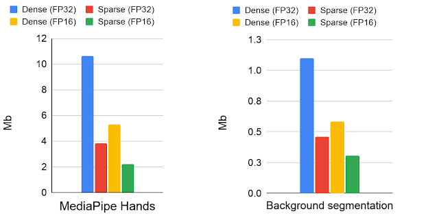
Model size comparisons for the dense and sparse models in Mb. The models have been stored in 16- and 32-bit floating-point formats.

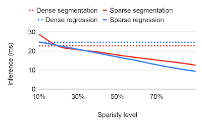
The approach to sparsity described here works best with architectures based on inverted residual blocks, such as MobileNetV2, MobileNetV3 and EfficientNetLite. The degree of sparsity in a network influences both inference speed and quality. Starting from a dense network of a fixed capacity, we found modest performance gains even at 30% sparsity. With increased sparsity, the quality of the model remains relatively close to the dense baseline until reaching 70% sparsity, beyond which there is a more pronounced drop in accuracy. However, one can compensate for the reduced accuracy at 70% sparsity by increasing the size of the base network by 20%, which results in faster inference times without degrading the quality of the model. No further changes are required to run the sparsified models, because XNNPACK can recognize and automatically enable sparse inference.

Ablation studies of different sparsity levels with respect to inference time (the smaller the better) and the quality measured by the Intersection over Union (IoU) for predicted segmentation mask.

Sparsity as Automatic Alternative to Distillation
Background blur in Google Meet uses a segmentation model based on a modified MobileNetV3 backbone with attention blocks. We were able to speed up the model by 30% by applying a 70% sparsification, while preserving the quality of the foreground mask. We examined the predictions of the sparse and dense models on images from 17 geographic subregions, finding no significant difference, and released the details in the associated model card.

Similarly, MediaPipe Hands predicts hand landmarks in real-time on mobile and the web using a model based on the EfficientNetLite backbone. This backbone model was manually distilled from the large dense model, which is a computationally expensive, iterative process. Using the sparse version of the dense model instead of distilled one, we were able to maintain the same inference speed but without the labor intensive process of distilling from a dense model. Compared with the dense model the sparse model improved the inference by a factor of two, achieving the identical landmark quality as the distilled model. In a sense, sparsification can be thought of as an automatic approach to unstructured model distillation, which can improve model performance without extensive manual effort. We evaluated the sparse model on the geodiverse dataset and made the model card publicly available.

Comparison of execution time for the dense (left), distilled (middle) and sparse (right) models of the same quality. Processing time of the dense model is 2x larger than sparse or distilled models. The distilled model is taken from the official MediPipe solution. The dense and sparse web demos are publicly available.

Future work
We find sparsification to be a simple yet powerful technique for improving CPU inference of neural networks. Sparse inference allows engineers to run larger models without incurring a significant performance or size overhead and offers a promising new direction for research. We are continuing to extend XNNPACK with wider support for operations in CHW layout and are exploring how it might be combined with other optimization techniques like quantization. We are excited to see what you might build with this technology!

Acknowledgments
Special thanks to all who worked on this project: Karthik Raveendran, Erich Elsen, Tingbo Hou‎, Trevor Gale, Siargey Pisarchyk, Yury Kartynnik, Yunlu Li, Utku Evci, Matsvei Zhdanovich, Sebastian Jansson, Stéphane Hulaud, Michael Hays, Juhyun Lee, Fan Zhang, Chuo-Ling Chang, Gregory Karpiak, Tyler Mullen, Jiuqiang Tang, Ming Guang Yong, Igor Kibalchich, and Matthias Grundmann.

Source: Google AI Blog


Uncovering Unknown Unknowns in Machine Learning

The performance of machine learning (ML) models depends both on the learning algorithms, as well as the data used for training and evaluation. The role of the algorithms is well studied and the focus of a multitude of challenges, such as SQuAD, GLUE, ImageNet, and many others. In addition, there have been efforts to also improve the data, including a series of workshops addressing issues for ML evaluation. In contrast, research and challenges that focus on the data used for evaluation of ML models are not commonplace. Furthermore, many evaluation datasets contain items that are easy to evaluate, e.g., photos with a subject that is easy to identify, and thus they miss the natural ambiguity of real world context. The absence of ambiguous real-world examples in evaluation undermines the ability to reliably test machine learning performance, which makes ML models prone to develop “weak spots”, i.e., classes of examples that are difficult or impossible for a model to accurately evaluate, because that class of examples is missing from the evaluation set.

To address the problem of identifying these weaknesses in ML models, we recently launched the Crowdsourcing Adverse Test Sets for Machine Learning (CATS4ML) Data Challenge at HCOMP 2020 (open until 30 April, 2021 to researchers and developers worldwide). The goal of the challenge is to raise the bar in ML evaluation sets and to find as many examples as possible that are confusing or otherwise problematic for algorithms to process. CATS4ML relies on people’s abilities and intuition to spot new data examples about which machine learning is confident, but actually misclassifies.

What are ML “Weak Spots”?
There are two categories of weak spots: known unknowns and unknown unknowns. Known unknowns are examples for which a model is unsure about the correct classification. The research community continues to study this in a field known as active learning, and has found the solution to be, in very general terms, to interactively solicit new labels from people on uncertain examples. For example, if a model is not certain whether or not the subject of a photo is a cat, a person is asked to verify; but if the system is certain, a person is not asked. While there is room for improvement in this area, what is comforting is that the confidence of the model is correlated with its performance, i.e., one can see what the model doesn’t know.

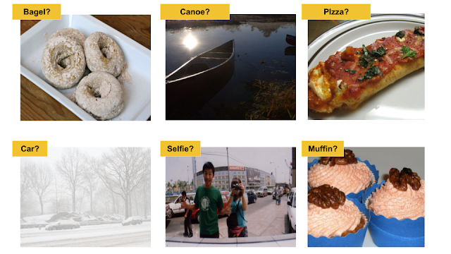
Unknown unknowns, on the other hand, are examples where a model is confident about its answer, but is actually wrong. Efforts to proactively discover unknown unknowns (e.g., Attenberg 2015 and Crawford 2019) have helped uncover a multitude of unintended machine behaviours. In contrast to such approaches for the discovery of unknown unknowns, generative adversarial networks (GANs) generate unknown unknowns for image recognition models in the form of optical illusions for computers that cause deep learning models to make mistakes beyond human perception. While GANs uncover model exploits in the event of an intentional manipulation, real-world examples can better highlight a model’s failures in its day-to-day performance. These real-world examples are the unknown unknowns of interest to CATS4ML — the challenge aims to gather unmanipulated examples that humans can reliably interpret but on which many ML models would confidently disagree.

Example illustrating how optical illusions for computers caused by adversarial noise help discover machine manipulated unknown unknowns for ML models (based on Brown 2018).

First Edition of CATS4ML Data Challenge: Open Images Dataset
The CATS4ML Data Challenge focuses on visual recognition, using images and labels from the Open Images Dataset. The target images for the challenge are selected from the Open Images Dataset along with a set of 24 target labels from the same dataset. The challenge participants are invited to invent new and creative ways to explore this existing publicly available dataset and, focussed on a list of pre-selected target labels, discover examples of unknown unknowns for ML models.

Examples from the Open Images Dataset as possible unknown unknowns for ML models.

CATS4ML is a complementary effort to FAIR’s recently introduced DynaBench research platform for dynamic data collection. Where DynaBench tackles issues with static benchmarks using ML models with humans in the loop, CATS4ML focuses on improving evaluation datasets for ML by encouraging the exploration of existing ML benchmarks for adverse examples that can be unknown unknowns. The results will help detect and avoid future errors, and also will give insights to model explainability.

In this way, CATS4ML aims to raise greater awareness of the problem by providing dataset resources that developers can use to uncover the weak spots of their algorithms. This will also inform researchers on how to create benchmark datasets for machine learning that are more balanced, diverse and socially aware.

Get Involved
We invite the global community of ML researchers and practitioners to join us in the effort of discovering interesting, difficult examples from the Open Images Dataset. Register on the challenge website, download the target images and labeled data, contribute the images you discover and join the competition for the winning participant!

To score points in this competition, participants should submit a set of image-label pairs that will be confirmed by human-in-the-loop raters, whose votes should be in disagreement with the average machine score for the label over a number of machine learning models.

An example of how a submitted image can score points. The same image can score as a false positive (Left) and as a false negative (Right) with two different labels. In both cases the human verification is in disagreement with the machine score. Participants score on submitted image-label pairs, which means that one and the same image can be an example of an ML unknown unknown for different labels.

The challenge is open until 30 April, 2021 to researchers and developers worldwide. To learn more about CATS4ML and how to join, please review these slides and visit the challenge website.

Acknowledgements
The release of the CATS4ML Data Challenge has been possible thanks to the hard work of a lot of people including, but not limited to, the following (in alphabetical order of last name): Osman Aka, Ken Burke, Tulsee Doshi, Mig Gerard, Victor Gomes, Shahab Kamali, Igor Karpov, Devi Krishna, Daphne Luong, Carey Radebaugh, Jamie Taylor, Nithum Thain, Kenny Wibowo, Ka Wong, and Tong Zhou.

Source: Google AI Blog


TracIn — A Simple Method to Estimate Training Data Influence

The quality of a machine learning (ML) model’s training data can have a significant impact on its performance. One measure of data quality is the notion of influence, i.e., the degree to which a given training example affects the model and its predictive performance. And while influence is a well-known concept to ML researchers, the complexity behind deep learning models, coupled with their growing size, features and datasets, have made the quantification of influence difficult.

A few methods have been proposed recently to quantify influence. Some rely on changes in accuracy when retraining with one or several data points dropped, and some use established statistical methods, e.g., influence functions that estimate the impact of perturbing input points or representer methods that decompose a prediction into an importance weighted combination of training examples. Still other approaches require use of additional estimators, such as data valuation using reinforcement learning. Though these approaches are theoretically sound, their use in products has been limited by the resources needed to run them at scale or the additional burdens they place on training.

In “Estimating Training Data Influence by Tracing Gradient Descent”, published as a spotlight paper at NeurIPS 2020, we proposed TracIn, a simple scalable approach to tackle this challenge. The idea behind TracIn is straightforward — trace the training process to capture changes in prediction as individual training examples are visited. TracIn is effective in finding mislabeled examples and outliers from a variety of datasets, and is useful in explaining predictions in terms of training examples (as opposed to features) by assigning an influence score to each training example.

The Ideas Underlying TracIn
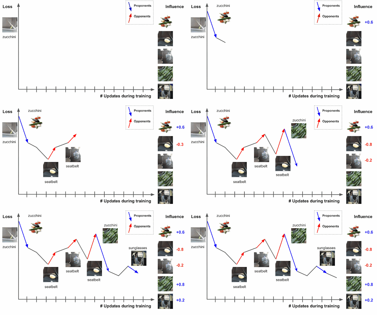
Deep learning algorithms are typically trained using an algorithm called stochastic gradient descent (SGD), or a variant of it. SGD operates by making multiple passes over the data and making modifications to the model parameters that locally reduce the loss (i.e., the model’s objective) with each pass. An example of this is demonstrated for an image classification task in the figure below, where the model’s task is to predict the subject of the test image on the left (“zucchini”). As the model progresses through training, it is exposed to various training examples that affect the loss on the test image, where the loss is a function both of the prediction score and the actual label — the higher the prediction score for zucchini, the lower the loss.

Estimating training data influence of the images on the right by tracing the loss change of the zucchini in the seatbelt image during training.

Suppose that the test example is known at training time and that the training process visited each training example one at a time. During the training, visiting a specific training example would change the model’s parameters, and that change would then modify the prediction/loss on the test example. If one could trace the training example through the process, then the change in loss or prediction on the test example could be attributed to the training example in question, where the influence of a training example would be the cumulative attribution across visits to the training example.

There are two types of relevant training examples. Those that reduce loss, like the images of zucchinis above, are called proponents, while those that increase loss, like the images of seatbelts, are called opponents. In the example above, the image labeled “sunglasses” is also a proponent, because it has a seatbelt in the image, but is labeled as “sunglasses,” driving the model to better distinguish between zucchini and seatbelts.

In practice, the test example is unknown at training time, a limitation that can be overcome by using the checkpoints output by the learning algorithm as a sketch of the training process. Another challenge is that the learning algorithm typically visits several points at once, not individually, which requires a method to disentangle the relative contributions of each training example. This can be done by applying pointwise loss gradients. Together, these two strategies capture the TracIn method, which can be reduced to the simple form of the dot product of loss gradients of the test and training examples, weighted by the learning rate, and summed across checkpoints.

The simple expression for TracIn influence. The dot product of loss gradients of training example (z) and test example (z') is weighted by learning rate (ηi) at different checkpoints and summed up.

Alternatively, one could instead examine the influence on the prediction score, which would be useful if the test example has no label. This form simply requires the substitution of the loss gradient at the test example with the prediction gradient.

Computing Top Influence Examples
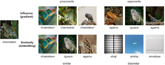
We illustrate the utility of TracIn by first calculating the loss gradient vector for some training data and a test example for a specific classification — an image of a chameleon — and then leveraging a standard k-nearest neighbors library to retrieve the top proponents and opponents. The top opponents indicate the chameleon’s ability to blend in! For comparison, we also show the k nearest neighbors with embeddings from the penultimate layer. Proponents are images that are not only similar, but also belong to the same class, and opponents are similar images but in a different class. Note that there isn’t an explicit enforcement on whether proponents or opponents belong to the same class.

Top row: Top proponents and opponents of influence vectors. Bottom row: Most similar and dissimilar examples of embedding vectors from the penultimate layer.

Clustering
The simplistic breakdown of the loss of the test example into training example influences given by TracIn also suggests that the loss (or prediction) from any gradient descent based neural model can be expressed as a sum of similarities in the space of gradients. Recent work has demonstrated that this functional form is similar to that of a kernel, implying that this gradient similarity described here can be applied to other similarity tasks, like clustering.

In this case, TracIn can be used as a similarity function within a clustering algorithm. To bound the similarity metric so that it can be converted to a distance measure (1 - similarity), we normalize the gradient vectors to have unit norm. Below, we apply TracIn clustering on images of zucchini to obtain finer clusters.

Finer clusters within Zucchini images using TracIn similarity. Each row is a cluster with zucchini in similar forms within the cluster: cross-sectionally sliced zucchini (top), piles of zucchinis (middle), and zucchinis on pizzas (bottom).

Identifying Outliers with Self-Influence
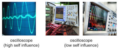
Finally, we can also use TracIn to identify outliers that exhibit a high self-influence, i.e., the influence of a training point on its own prediction. This happens either when the example is mislabeled or rare, both of which make it difficult for the model to generalize over the example. Below are some examples with high self-influence.

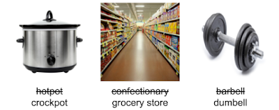
Mislabeled examples. Assigned labels are striked out, correct labels are at bottom.
Left: A rare oscilloscope example with just the oscillations, and no instrument in the image gets high self-influence. Right: Other common oscilloscope images have the scope with knobs and wires. These have a low self-influence.

Applications
Having no requirement other than being trained using SGD (or related variants), TracIn is task-independent and applicable to a variety of models. For example, we have used TracIn to study training data for a deep learning model used to parse queries to the Google Assistant, queries of the kind “set my alarm for 7AM”. We were intrigued to see that the top opponent for the query “disable my alarm” with an alarm active on the device, was “disable my timer”, also with an alarm active on the device. This suggests that Assistant users often interchange the words “timer” and “alarm”. TracIn helped us interpret the Assistant data.

More examples can be found in the paper, including a regression task on structured data and a number of text classification tasks.

Conclusion
TracIn is a simple, easy-to-implement, scalable way to compute the influence of training data examples on individual predictions or to find rare and mislabeled training examples. For implementation references of the method, you can find a link to code examples for images from the github linked in the paper.

Acknowledgements
The NeurIPS paper was jointly co-authored with Satyen Kale and Mukund Sundararajan (corresponding author). A special thanks to Binbin Xiong for providing various conceptual and implementation insights. We also thank Qiqi Yan and Salem Haykal for numerous discussions. Images throughout this post sourced from Getty Images.

Source: Google AI Blog


Machine Learning for Computer Architecture

One of the key contributors to recent machine learning (ML) advancements is the development of custom accelerators, such as Google TPUs and Edge TPUs, which significantly increase available compute power unlocking various capabilities such as AlphaGo, RankBrain, WaveNets, and Conversational Agents. This increase can lead to improved performance in neural network training and inference, enabling new possibilities in a broad range of applications, such as vision, language, understanding, and self-driving cars.

To sustain these advances, the hardware accelerator ecosystem must continue to innovate in architecture design and acclimate to rapidly evolving ML models and applications. This requires the evaluation of many different accelerator design points, each of which may not only improve the compute power, but also unravel a new capability. These design points are generally parameterized by a variety of hardware and software factors (e.g., memory capacity, number of compute units at different levels, parallelism, interconnection networks, pipelining, software mapping, etc.). This is a daunting optimization task, due to the fact that the search space is exponentially large1 while the objective function (e.g., lower latency and/or higher energy efficiency) is computationally expensive to evaluate through simulations or synthesis, making identification of feasible accelerator configurations challenging .

In “Apollo: Transferable Architecture Exploration”, we present the progress of our research on ML-driven design of custom accelerators. While recent work has demonstrated promising results in leveraging ML to improve the low-level floorplanning process (in which the hardware components are spatially laid out and connected in silicon), in this work we focus on blending ML into the high-level system specification and architectural design stage, a pivotal contributing factor to the overall performance of the chip in which the design elements that control the high-level functionality are established. Our research shows how ML algorithms can facilitate architecture exploration and suggest high-performing architectures across a range of deep neural networks, with domains spanning image classification, object detection, OCR and semantic segmentation.

Architecture Search Space and Workloads
The objective in architecture exploration is to discover a set of feasible accelerator parameters for a set of workloads, such that a desired objective function (e.g., the weighted average of runtime) is minimized under an optional set of user-defined constraints. However, the manifold of architecture search generally contains many points for which there is no feasible mapping from software to hardware. Some of these design points are known a priori and can be bypassed by formulating them as optimization constraints by the user (e.g., in the case of an area budget2 constraint, the total memory size must not pass over a predefined limit). However, due to the interplay of the architecture and compiler and the complexity of the search space, some of the constraints may not be properly formulated into the optimization, and so the compiler may not find a feasible software mapping for the target hardware. These infeasible points are not easy to formulate in the optimization problem, and are generally unknown until the whole compiler pass is performed. As such, one of main challenges for architecture exploration is to effectively sidestep the infeasible points for efficient exploration of the search space with a minimum number of cycle-accurate architecture simulations.

The following figure shows the overall architecture search space of a target ML accelerator. The accelerator contains a 2D array of processing elements (PE), each of which performs a set of arithmetic computations in a single instruction multiple data (SIMD) manner. The main architectural components of each PE are processing cores that include multiple compute lanes for SIMD operations. Each PE has shared memory (PE Memory) across all their compute cores, which is mainly used to store model activations, partial results, and outputs, while individual cores feature memory that is mainly used for storing model parameters. Each core has multiple compute lanes with multi-way multiply-accumulate (MAC) units. The results of model computations at each cycle are either stored back in the PE memory for further computation or are offloaded back into the DRAM.

Overview of the template-based ML accelerator used for architecture exploration.

Optimization Strategies
In this study, we explored four optimization strategies in the context of architecture exploration:

  1. Random:Samples the architecture search space uniformly at random.
  2. Vizier: Uses Bayesian optimization for the exploration in the search space in which the evaluation of the objective function is expensive (e.g. hardware simulation which can take hours to complete). Using a collection of sampled points from the search space, the Bayesian optimization forms a surrogate function, usually represented by a Gaussian process, that approximates the manifold of the search space. Guided by the value of the surrogate function, the Bayesian optimization algorithm decides, in an exploration and exploitation trade-off, whether to sample more from the promising regions in the manifold (exploitation) or sample more from the unseen regions in the search space (exploration). Then, the optimization algorithm uses these newly sampled points and further updates the surrogate function to better model the target search space. Vizier uses expected improvement as its core acquisition function.
  3. Evolutionary: Performs evolutionary search using a population of k individuals, where the genome of each individual corresponds to a sequence of discretized accelerator configurations. New individuals are generated by selecting for each individual two parents from the population using tournament selecting, recombining their genomes with some crossover rate, and mutating the recombined genome with some probability.
  4. Population-based black-box optimization (P3BO): Uses an ensemble of optimization methods, including evolutionary and model-based, which has been shown to increase sample-efficiency and robustness. The sampled data are exchanged between optimization methods in the ensemble, and optimizers are weighted by their performance history to generate new configurations. In our study, we use a variant of P3BO in which the hyper-parameters of the optimizers are dynamically updated using evolutionary search.

Accelerator Search Space Embeddings
To better visualize the effectiveness of each optimization strategy in navigating the accelerator search space, we use t-distributed stochastic neighbor embedding (t-SNE) to map the explored configurations into a two-dimensional space across the optimization horizon. The objective (reward) for all the experiments is defined as the throughput (inference/second) per accelerator area. In the figures below, the x and y axes indicate the t-SNE components (embedding 1 and embedding 2) of the embedding space. The star and circular markers show the infeasible (zero reward) and feasible design points, respectively, with the size of the feasible points corresponding to their reward.

As expected, the random strategy searches the space in a uniformly distributed way and eventually finds very few feasible points in the design space.

Visualization presenting the t-SNE of the explored design points (~4K) by random optimization strategy (max reward = 0.96). The maximum reward points (red cross markers) are highlighted at the last frame of the animation.

Compared to the random sampling approach, the Vizier default optimization strategy strikes a good balance between exploring the search space and finding the design points with higher rewards (1.14 vs. 0.96). However, this approach tends to get stuck in infeasible regions and, while it does find a few points with the maximum reward (indicated by the red cross markers), it finds few feasible points during the last iterations of exploration.

As above, with the Vizier (default) optimization strategy (max reward = 1.14). The maximum reward points (red cross markers) are highlighted at the last frame of the animation.

The evolutionary optimization strategy, on the other hand, finds feasible solutions very early in the optimization and assemble clusters of feasible points around them. As such, this approach mostly navigates the feasible regions (the green circles) and efficiently sidesteps the infeasible points. In addition, the evolutionary search is able to find more design options with maximum reward (the red crosses). This diversity in the solutions with high reward provides flexibility to the designer in exploring various architectures with different design trade-offs.

As above, with the evolutionary optimization strategy (max reward = 1.10). The maximum reward points (red cross markers) are highlighted at the last frame of the animation.

Finally, the population-based optimization method (P3BO) explores the design space in a more targeted way (regions with high reward points) in order to find optimal solutions. The P3BO strategy finds design points with the highest reward in search spaces with tighter constraints (e.g., a larger number of infeasible points), showing its effectiveness in navigating search spaces with large numbers of infeasible points.

As above, with the P3BO optimization strategy (max reward = 1.13). The maximum reward points (red cross markers) are highlighted at the last frame of the animation.

Architecture Exploration under Different Design Constraints
We also studied the benefits of each optimization strategy under different area budget constraints, 6.8 mm2, 5.8 mm2 and 4.8 mm2. The following violin plots show the full distribution of the maximum achievable reward at the end of optimization (after ten runs each with 4K trials) across the studied optimization strategies. The wider sections represent a higher probability of observing feasible architecture configurations at a particular given reward. This implies that we favor the optimization algorithm that yields increased width at the points with higher reward (higher performance).

The two top-performing optimization strategies for architecture exploration are evolutionary and P3BO, both in terms of delivering solutions with high reward and robustness across multiple runs. Looking into different design constraints, we observe that as one tightens the area budget constraint, the P3BO optimization strategy yields more high performing solutions. For example, when the area budget constraint is set to 5.8 mm2, P3BO finds design points with a reward (throughput / accelerator area) of 1.25 outperforming all the other optimization strategies. The same trend is observed when the area budget constraint is set to 4.8 mm2, a slightly better reward is found with more robustness (less variability) across multiple runs.

Violin plot showing the full distribution of the maximum achievable reward in ten runs across the optimization strategies after 4K trial evaluations under an area budget of 6.8 mm2. The P3BO and Evolutionary algorithm yield larger numbers of high-performing designs (wider sections). The x and y axes indicate the studied optimization algorithms and the geometric mean of speedup (reward) over the baseline accelerator, respectively.
As above, under an area budget of 5.8 mm2.
As above, under an area budget of 4.8 mm2.

Conclusion
While Apollo presents the first step towards better understanding of accelerator design space and building more efficient hardware, inventing accelerators with new capabilities is still an uncharted territory and a new frontier. We believe that this research is an exciting path forward to further explore ML-driven techniques for architecture design and co-optimization (e.g., compiler, mapping, and scheduling) across the computing stack to invent efficient accelerators with new capabilities for the next generation of applications.

Acknowledgments
This work was performed by Amir Yazdanbakhsh, Christof Angermueller, and Berkin Akin . We would like to also thank Milad Hashemi, Kevin Swersky, James Laudon, Herman Schmit, Cliff Young, Yanqi Zhou, Albin Jones, Satrajit Chatterjee, Ravi Narayanaswami, Ray (I-Jui) Sung, Suyog Gupta, Kiran Seshadri, Suvinay Subramanian, Matthew Denton, and the Vizier team for their help and support.


1 In our target accelerator, the total number of design points is around 5 x 10⁸

2 The chip area is approximately the sum of total hardware components on the chip, including on-chip storage, processing engines, controllers, I/O pins, and etc.  

Source: Google AI Blog


Recognizing Pose Similarity in Images and Videos

Everyday actions, such as jogging, reading a book, pouring water, or playing sports, can be viewed as a sequence of poses, consisting of the position and orientation of a person’s body. An understanding of poses from images and videos is a crucial step for enabling a range of applications, including augmented reality display, full-body gesture control, and physical exercise quantification. However, a 3-dimensional pose captured in two dimensions in images and videos appears different depending on the viewpoint of the camera. The ability to recognize similarity in 3D pose using only 2D information will help vision systems better understand the world.

In “View-Invariant Probabilistic Embedding for Human Pose” (Pr-VIPE), a spotlight paper at ECCV 2020, we present a new algorithm for human pose perception that recognizes similarity in human body poses across different camera views by mapping 2D body pose keypoints to a view-invariant embedding space. This ability enables tasks, such as pose retrieval, action recognition, action video synchronization, and more. Compared to existing models that directly map 2D pose keypoints to 3D pose keypoints, the Pr-VIPE embedding space is (1) view-invariant, (2) probabilistic in order to capture 2D input ambiguity, and (3) does not require camera parameters during training or inference. Trained with in-lab setting data, the model works on in-the-wild images out of the box, given a reasonably good 2D pose estimator (e.g., PersonLab, BlazePose, among others). The model is simple, results in compact embeddings, and can be trained (in ~1 day) using 15 CPUs. We have released the code on our GitHub repo.

Pr-VIPE can be directly applied to align videos from different views.

Pr-VIPE
The input to Pr-VIPE is a set of 2D keypoints, from any 2D pose estimator that produces a minimum of 13 body keypoints, and the output is the mean and variance of the pose embedding. The distances between embeddings of 2D poses correlate to their similarities in absolute 3D pose space. Our approach is based on two observations:

  • The same 3D pose may appear very different in 2D as the viewpoint changes.
  • The same 2D pose can be projected from different 3D poses.

The first observation motivates the need for view-invariance. To accomplish this, we define the matching probability, i.e., the likelihood that different 2D poses were projected from the same, or similar 3D poses. The matching probability predicted by Pr-VIPE for matching pose pairs should be higher than for non-matching pairs.

To address the second observation, Pr-VIPE utilizes a probabilistic embedding formulation. Because many 3D poses can project to the same or similar 2D poses, the model input exhibits an inherent ambiguity that is difficult to capture through deterministic mapping point-to-point in embedding space. Therefore, we map a 2D pose through a probabilistic mapping to an embedding distribution, of which we use the variance to represent the uncertainty of the input 2D pose. As an example, in the figure below the third 2D view of the 3D pose on the left is similar to the first 2D view of a different 3D pose on the right, so we map them into a similar location in the embedding space with large variances.

Pr-VIPE enables vision systems to recognize 2D poses across views. We embed 2D poses using Pr-VIPE such that the embeddings are (1) view-invariant (2D projections of similar 3D poses are embedded close together) and (2) probabilistic. By embedding detected 2D poses, Pr-VIPE enables direct retrieval of pose images from different views, and can also be applied to action recognition and video alignment.
View-Invariance
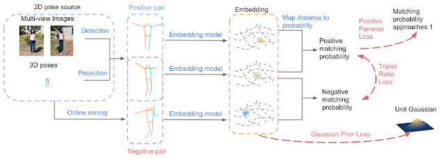
During training, we use 2D poses from two sources: multi-view images and projections of groundtruth 3D poses. Triplets of 2D poses (anchor, positive, and negative) are selected from a batch, where the anchor and positive are two different projections of the same 3D pose, and the negative is a projection of a non-matching 3D pose. Pr-VIPE then estimates the matching probability of 2D pose pairs from their embeddings.
During training, we push the matching probability of positive pairs to be close to 1 with a positive pairwise loss in which we minimize the embedding distance between positive pairs, and the matching probability of negative pairs to be small by maximizing the ratio of the matching probabilities between positive and negative pairs with a triplet ratio loss.
Overview of the Pr-VIPE model. During training, we apply three losses (triplet ratio loss, positive pairwise loss, and a prior loss that applies a unit Gaussian prior to our embeddings). During inference, the model maps an input 2D pose to a probabilistic, view-invariant embedding.
Probabilistic Embedding
Pr-VIPE maps a 2D pose to a probabilistic embedding as a multivariate Gaussian distribution using a sampling-based approach for similarity score computation between two distributions. During training, we use a Gaussian prior loss to regularize the predicted distribution.

Evaluation
We propose a new cross-view pose retrieval benchmark to evaluate the view-invariance property of the embedding. Given a monocular pose image, cross-view retrieval aims to retrieve the same pose from different views without using camera parameters. The results demonstrate that Pr-VIPE retrieves poses more accurately across views compared to baseline methods in both evaluated datasets (Human3.6M, MPI-INF-3DHP).

Pr-VIPE retrieves poses across different views more accurately relative to the baseline method (3D pose estimation).

Common 3D pose estimation methods (such as the simple baseline used for comparison above, SemGCN, and EpipolarPose, amongst many others), predict 3D poses in camera coordinates, which are not directly view-invariant. Thus, rigid alignment between every query-index pair is required for retrieval using estimated 3D poses, which is computationally expensive due to the need for singular value decomposition (SVD). In contrast, Pr-VIPE embeddings can be directly used for distance computation in Euclidean space, without any post-processing.

Applications
View-invariant pose embedding can be applied to many image and video related tasks. Below, we show Pr-VIPE applied to cross-view retrieval on in-the-wild images without using camera parameters.


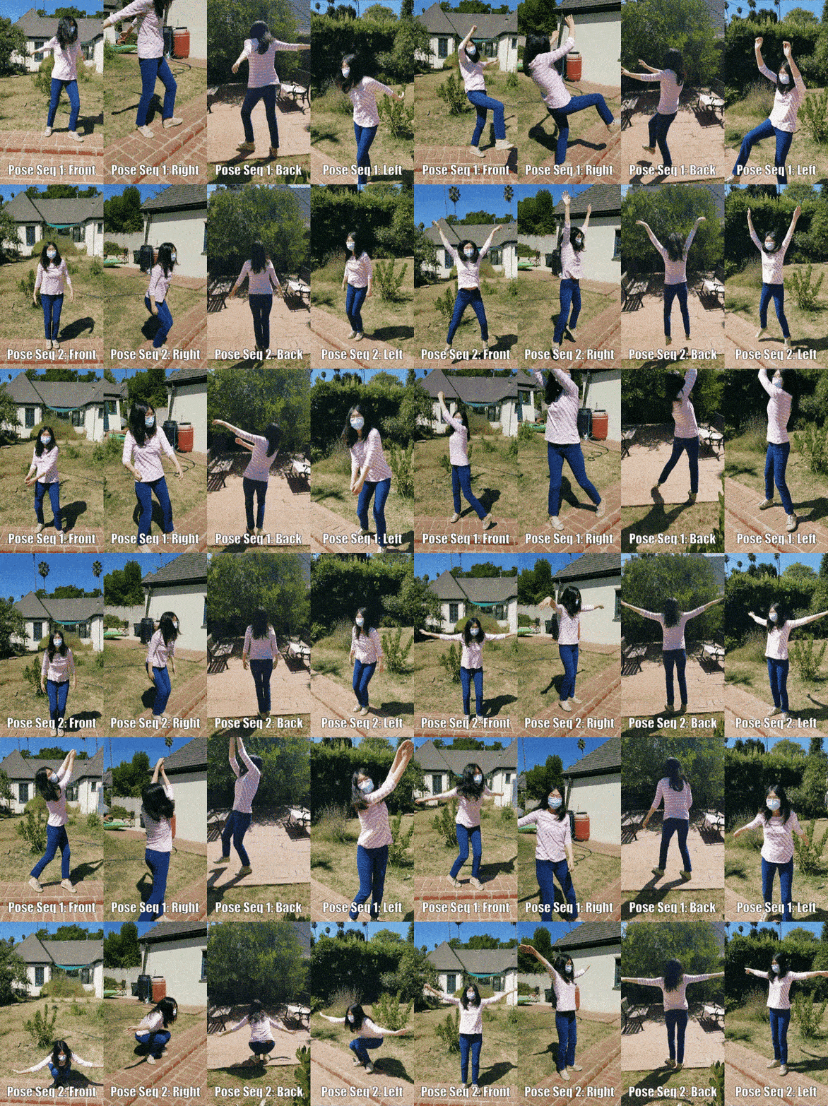
We can retrieve in-the-wild images from different views without using camera parameters by embedding the detected 2D pose using Pr-VIPE. Using the query image (top row), we search for a matching pose from a different camera view and we show the nearest neighbor retrieval (bottom row). This enables us to search for matching poses across camera views more easily.

The same Pr-VIPE model can also be used for video alignment. To do so, we stack Pr-VIPE embeddings within a small time window, and use the dynamic time warping (DTW) algorithm to align video pairs.

Manual video alignment is difficult and time-consuming. Here, Pr-VIPE is applied to automatically align videos of the same action repeated from different views.

The video alignment distance calculated via DTW can then be used for action recognition by classifying videos using nearest neighbor search. We evaluate the Pr-VIPE embedding using the Penn Action dataset and demonstrate that using the Pr-VIPE embedding without fine-tuning on the target dataset, yields highly competitive recognition accuracy. In addition, we show that Pr-VIPE even achieves relatively accurate results using only videos from a single view in the index set.

Pr-VIPE recognizes action across views using pose inputs only, and is comparable to or better than methods using pose only or with additional context information (such as Iqbal et al., Liu and Yuan, Luvizon et al., and Du et al.). When action labels are only available for videos from a single view, Pr-VIPE (1-view only) can still achieve relatively accurate results.

Conclusion
We introduce the Pr-VIPE model for mapping 2D human poses to a view-invariant probabilistic embedding space, and show that the learned embeddings can be directly used for pose retrieval, action recognition, and video alignment. Our cross-view retrieval benchmark can be used to test the view-invariant property of other embeddings. We look forward to hearing about what you can do with pose embeddings!

Acknowledgments
Special thanks to Jiaping Zhao, Liang-Chieh Chen, Long Zhao (Rutgers University), Liangzhe Yuan, Yuxiao Wang, Florian Schroff, Hartwig Adam, and the Mobile Vision team for the wonderful collaboration and support.

Source: Google AI Blog


“L10n” – Localisation: Breaking down language barriers to unleash the benefits of the internet for all Indians

In July, at the Google for India event, we outlined our vision to make the Internet helpful for a billion Indians, and power the growth of India’s digital economy. One critical area that we need to overcome is the challenge of India’s vast linguistic diversity, with dialects changing every hundred kilometres. More often than not, one language doesn’t seamlessly map to another. A word in Bengali roughly translates to a full sentence in Tamil and there are expressions in Urdu which have no adequately evocative equivalent in Hindi. 


This poses a formidable challenge for technology developers, who rely on commonly understood visual and spoken idioms to make tech products work universally. 


We realised early on that there was no way to simplify this challenge - that there wasn’t any one common minimum that could address the needs of every potential user in this country. If we hoped to bring the potential of the internet within reach of every user in India, we had to invest in building products, content and tools in every popularly spoken Indian language. 


India’s digital transformation will be incomplete if English proficiency continues to be the entry barrier for basic and potent uses of the Internet such as buying and selling online, finding jobs, using net banking and digital payments or getting access to information and registering for government schemes.


The work, though underway, is far from done. We are driving a 3-point strategy to truly digitize India:


  1. Invest in ML & AI efforts at Google’s research center in India, to make advances in machine learning and AI models accessible to everyone across the ecosystem.

  2. Partner with innovative local startups who are building solutions to cater to the needs of Indians in local languages

  3. Drastically improve the experience of Google products and services for Indian language users


And so today, we are happy to announce a range of features to help deliver an even richer language experience to millions across India.

Easily toggling between English and Indian language results

Four years ago we made it easier for people in states with a significant Hindi-speaking population to flip between English and Hindi results for a search query, by introducing a simple ‘chip’ or tab they could tap to see results in their preferred language. In fact, since the launch of this Hindi chip and other language features, we have seen more than a 10X increase in Hindi queries in India.

We are now making it easier to toggle Search results between English and four additional Indian languages: Tamil, Telugu, Bangla and Marathi.

People can now tap a chip to see Search results in their local language

Understanding which language content to surface, when

Typing in an Indian language in its native script is typically more difficult, and can often take three times as long, compared to English. As a result, many people search in English even if they really would prefer to see results in a local language they understand.

Search will show relevant results in more Indian languages

Over the next month, Search will start to show relevant content in supported Indian languages where appropriate, even if the local language query is typed in English. This functionality will also better serve bilingual people who are comfortable reading both English and an Indian language. It will roll out in five Indian languages: Hindi, Bangla, Marathi, Tamil, and Telugu.

Enabling people to use apps in the language of their choice

Just like you use different tools for different tasks, we know (because we do it ourselves) people often select a specific language for a particular situation. Rather than guessing preferences, we launched the ability to easily change the language of Google Assistant and Discover to be different from the phone language. Today in India, more than 50 percent of the content viewed on Google Discover is in Indian languages. A third of Google Assistant users in India are using it in an Indian language, and since the launch of Assistant language picker, queries in Indian languages have doubled.

Maps will now able people to select up to nine Indian languages

We are now extending this ability to Google Maps, where users can quickly and easily change their Maps experience into one of nine Indian languages, by simply opening the app, going to Settings, and tapping ‘App language’. This will allow anyone to search for places, get directions and navigation, and interact with the Map in their preferred local language.

Homework help in Hindi (and English)

Meaning is also communicated with images: and this is where Google Lens can help. From street signs to restaurant menus, shop names to signboards, Google Lens lets you search what you see, get things done faster, and understand the world around you—using just your camera or a photo. In fact more people use Google Lens in India every month than in any other country worldwide. As an example of its popularity, over 3 billion words have been translated in India with Lens in 2020.

Lens is particularly helpful for students wanting to learn about the world. If you’re a parent, you’ll be familiar with your kids asking you questions about homework. About stuff you never thought you’d need to remember, like... quadratic equations.

Google Lens can now help you solve math problems by simply pointing your camera 

Now, right from the Search bar in the Google app, you can use Lens to snap a photo of a math problem and learn how to solve it on your own, in Hindi (or English). To do this, Lens first turns an image of a homework question into a query. Based on the query, we will show step-by-step guides and videos to help explain the problem.

Helping computer systems understand Indian languages at scale

At Google Research India, we have spent a lot of time helping computer systems understand human language. As you can imagine, this is quite an exciting challenge.The new approach we developed in India is called Multilingual Representations for Indian Languages (or ‘MuRIL’). Among many other benefits of this powerful multilingual model that scales across languages, MuRIL also provides support for transliterated text such as when writing Hindi using Roman script, which was something missing from previous models of its kind. 

One of the many tasks MuRIL is good at, is determining the sentiment of the sentence. For example, “Achha hua account bandh nahi hua” would previously be interpreted as having a negative meaning, but MuRIL correctly identifies this as a positive statement. Or take the ability to classify a person versus a place: ‘Shirdi ke sai baba’ would previously be interpreted as a place, which is wrong, but MuRIL correctly interprets it as a person.

MuRIL currently supports 16 Indian languages as well as English -- the highest coverage for Indian languages among any other publicly available model of its kind.

MuRIL is free & Open Source,

available on TensorFlow Hub

https://tfhub.dev/google/MuRIL/1


We are thrilled to announce that we have made MuRIL open source, and it is currently available to download from the TensorFlow Hub, for free. We hope MuRIL will be the next big evolution for Indian language understanding, forming a better foundation for researchers, students, startups, and anyone else interested in building Indian language technologies, and we can’t wait to see the many ways the ecosystem puts it to use.

We’re sharing this to provide a flavor of the depth of work underway -- and which is required -- to really make a universally potent and accessible Internet a reality. This said, the Internet in India is the sum of the work of millions of developers, content creators, news media and online businesses, and it is only when this effort is undertaken at scale by the entire ecosystem, that we will help fulfil the truly meaningful promise of the billionth Indian coming online.

Posted by the Google India team


Privacy Considerations in Large Language Models

Machine learning-based language models trained to predict the next word in a sentence have become increasingly capable, common, and useful, leading to groundbreaking improvements in applications like question-answering, translation, and more. But as language models continue to advance, new and unexpected risks can be exposed, requiring the research community to proactively work to develop new ways to mitigate potential problems.

One such risk is the potential for models to leak details from the data on which they’re trained. While this may be a concern for all large language models, additional issues may arise if a model trained on private data were to be made publicly available. Because these datasets can be large (hundreds of gigabytes) and pull from a range of sources, they can sometimes contain sensitive data, including personally identifiable information (PII) — names, phone numbers, addresses, etc., even if trained on public data. This raises the possibility that a model trained using such data could reflect some of these private details in its output. It is therefore important to identify and minimize the risks of such leaks, and to develop strategies to address the issue for future models.

If one prompts the GPT-2 language model with the prefix “East Stroudsburg Stroudsburg...”, it will autocomplete a long block of text that contains the full name, phone number, email address, and physical address of a particular person whose information was included in GPT-2’s training data.

In “Extracting Training Data from Large Language Models”, a collaboration with OpenAI, Apple, Stanford, Berkeley, and Northeastern University, we demonstrate that, given only the ability to query a pre-trained language model, it is possible to extract specific pieces of training data that the model has memorized. As such, training data extraction attacks are realistic threats on state-of-the-art large language models. This research represents an early, critical step intended to inform researchers about this class of vulnerabilities, so that they may take steps to mitigate these weaknesses.

Ethics of Language Model Attacks
A training data extraction attack has the greatest potential for harm when applied to a model that is available to the public, but for which the dataset used in training is not. However, since conducting this research on such a dataset could have harmful consequences, we instead mount a proof of concept training data extraction attack on GPT-2, a large, publicly available language model developed by OpenAI, that was trained using only public data. While this work focuses on GPT-2 specifically, the results apply to understanding what privacy threats are possible on large language models generally.

As with other privacy- and security-related research, it is important to consider the ethics of such attacks before actually performing them. To minimize the potential risk of this work, the training data extraction attack in this work was developed using publicly available data. Furthermore, the GPT-2 model itself was made public by OpenAI in 2019, and the training data used to train GPT-2 was collected from the public internet, and is available for download by anyone who follows the data collection process documented in the GPT-2 paper.

Additionally, in accordance with responsible computer security disclosure norms, we followed up with individuals whose PII was extracted, and secured their permission before including references to this data in publication. Further, in all publications of this work, we have redacted any personally identifying information that may identify individuals. We have also worked closely with OpenAI in the analysis of GPT-2.

The Training Data Extraction Attack
By design, language models make it very easy to generate a large amount of output data. By seeding the model with random short phrases, the model can generate millions of continuations, i.e., probable phrases that complete the sentence. Most of the time, these continuations will be benign strings of sensible text. For example, when asked to predict the continuation of the string “Mary had a little…”, a language model will have high confidence that the next token is the word “lamb”. However, if one particular training document happened to repeat the string “Mary had a little wombat” many times, the model might predict that phrase instead.

The goal of a training data extraction attack is then to sift through the millions of output sequences from the language model and predict which text is memorized. To accomplish this, our approach leverages the fact that models tend to be more confident on results captured directly from their training data. These membership inference attacks enable us to predict if a result was used in the training data by checking the confidence of the model on a particular sequence.

The main technical contribution of this work is the development of a method for inferring membership with high accuracy along with techniques for sampling from models in a way that encourages the output of memorized content. We tested a number of different sampling strategies, the most successful of which generates text conditioned on a wide variety of input phrases. We then compare the output of two different language models. When one model has high confidence in a sequence, but the other (equally accurate) model has low confidence in a sequence, it's likely that the first model has memorized the data.

Results
Out of 1800 candidate sequences from the GPT-2 language model, we extracted over 600 that were memorized from the public training data, with the total number limited by the need for manual verification. The memorized examples cover a wide range of content, including news headlines, log messages, JavaScript code, PII, and more. Many of these examples are memorized even though they appear infrequently in the training dataset. For example, for many samples of PII we extract are found in only a single document in the dataset. However, in most of these cases, the originating document contains multiple instances of the PII, and as a result, the model still learns it as high likelihood text.

Finally, we also find that the larger the language model, the more easily it memorizes training data. For example, in one experiment we find that the 1.5 billion parameter GPT-2 XL model memorizes 10 times more information than the 124 million parameter GPT-2 Small model. Given that the research community has already trained models 10 to 100 times larger, this means that as time goes by, more work will be required to monitor and mitigate this problem in increasingly large language models.

Lessons
While we demonstrate these attacks on GPT-2 specifically, they show potential flaws in all large generative language models. The fact that these attacks are possible has important consequences for the future of machine learning research using these types of models.

Fortunately, there are several ways to mitigate this issue. The most straightforward solution is to ensure that models do not train on any potentially problematic data. But this can be difficult to do in practice.

The use of differential privacy, which allows training on a dataset without revealing any details of individual training examples, is one of the most principled techniques to train machine learning models with privacy. In TensorFlow, this can be achieved with the use of the tensorflow/privacy module (or similar for PyTorch or JAX) that is a drop-in replacement for existing optimizers. Even this can have limitations and won’t prevent memorization of content that is repeated often enough. If this is not possible, we recommend at least measuring how much memorization occurs so appropriate action can be taken.

Language models continue to demonstrate great utility and flexibility—yet, like all innovations, they can also pose risks. Developing them responsibly means proactively identifying those risks and developing ways to mitigate them. We hope that this effort to highlight current weaknesses in large language modeling will raise awareness of this challenge in the broader machine learning community and motivate researchers to continue to develop effective techniques to train models with reduced memorization.

Acknowledgements
This work was performed jointly with Florian Tramer, Eric Wallace, Matthew Jagielski, Ariel Herbert-Voss, Katherine Lee, Adam Roberts, Tom Brown, Dawn Song, Ulfar Erlingsson, Alina Oprea, and Colin Raffel.

Source: Google AI Blog


Announcing the Newest Addition to MLKit: Entity Extraction

Posted by Kenny Sulaimon, Product Manager, ML Kit, Tory Voight, Product Manager, ML Kit, Daniel Furlong, Lei Yu, Software Engineers, ML Kit, Dong Chen, Technical Lead, MLKit
ML Kit logo

Six months ago, we introduced the standalone version of the ML Kit SDK, making it even easier to integrate on-device machine learning into mobile apps. Since then, we’ve launched the Digital Ink Recognition and Pose Detection APIs, and also introduced the ML Kit early access program. Today we are excited to add Entity Extraction to the official ML Kit lineup and also debut a new API for our early access program, Selfie Segmentation!

Overview of ML Kit's Entity Extraction API

With ML Kit’s Entity Extraction API, you can now improve the user experience inside your app by understanding text and performing specific actions on it.

The Entity Extraction API allows you to detect and locate entities from raw text, and take action based on those entities. The API works on static text and also in real-time while a user is typing. It supports 11 different entities and 15 different languages (with more coming in the future) to allow developers to make any text interaction a richer experience for the user.

Supported Entities

  • Address (350 third street, cambridge)
  • Date-Time* (12/12/2020, tomorrow at 3pm) (let's meet tomorrow at 6pm)
  • Email ([email protected])
  • Flight Number* (LX37)
  • IBAN* (CH52 0483 0000 0000 0000 9)
  • ISBN* (978-1101904190)
  • Money (including currency)* ($12, 25USD)
  • Payment Card* (4111 1111 1111 1111)
  • Phone Number ((555) 225-3556, 12345)
  • Tracking Number* (1Z204E380338943508)
  • URL (www.google.com, https://en.wikipedia.org/wiki/Platypus, seznam.cz)
Example Results
Table of Input text and Detected entities

Real World Applications

2 phones showing TamTam using Entity Extraction API

(Images courtesy of TamTam)

Our early access partner, TamTam, has been using the Entity Extraction API to provide helpful suggestions to their users during their chat conversations. This feature allows users to quickly perform actions based on the context of their conversations.

While integrating this API, Iurii Dorofeev, Head of TamTam Android Development, mentioned, “We appreciated the ease of integration of the ML Kit ... and it works offline. Clustering the content of messages right on the device allowed us to save resources. ML Kit capabilities will help us develop other features for TamTam messenger in the future.”

Check out their messaging app on the Google Play and App Store today.

Under The Hood

Diagram of underlying Text Classifier API

(Diagram of underlying Text Classifier API)

ML Kit’s Entity Extraction API builds upon the technology powering the Smart Linkify feature in Android 10+ to deliver an easy-to-use and streamlined experience for developers. For an in-depth review of the Text Classifier API, please see our blog post here.

The neural network annotators/models in the Entity Extraction API work as follows: A given input text is first split into words (based on space separation), then all possible word subsequences of certain maximum length (15 words in the example above) are generated, and for each candidate the scoring neural net assigns a value (between 0 and 1) based on whether it represents a valid entity.

Next, the generated entities that overlap are removed, favoring the ones with a higher score over the conflicting ones with a lower score. Then a second neural network is used to classify the type of the entity as a phone number, an address, or in some cases, a non-entity.

The neural network models in the Entity Extraction API are used in combination with other types of models (e.g. rule-based) to identify additional entities in text, such as: flight numbers, currencies and other examples listed above. Therefore, if multiple entities are detected for one text input, the Entity Extraction API can return several overlapping results.

Lastly, ML Kit will automatically download the required language-specific models to the device dynamically. You can also explicitly manage models you want available on the device by using ML Kit’s model management API. This can be useful if you want to download models ahead of time for your users. The API also allows you to delete models that are no longer required.

New APIs Coming Soon

Selfie Segmentation

With the increased usage of selfie cameras and webcams in today's world, being able to quickly and easily add effects to camera experiences has become a necessity for many app developers today.

ML Kit's Selfie Segmentation API allows developers to easily separate the background from a scene and focus on what matters. Adding cool effects to selfies or inserting your users into interesting background environments has never been easier. This API produces great results with low latency on both Android and iOS devices.

Example of ML Kit Selfie Segmentation

(Example of ML Kit Selfie Segmentation)

Key capabilities:

  • Easily allows developers to replace or blur a user’s background
  • Works well with single or multiple people
  • Cross-platform support (iOS and Android)
  • Runs real-time on most modern phones

To join our early access program and request access to ML Kit's Selfie Segmentation API, please fill out this form.