Tag Archives: machine learning

Decisiveness in Imitation Learning for Robots

Posted by Pete Florence, Research Scientist and Corey Lynch, Research Engineer, Robotics at Google

Despite considerable progress in robot learning over the past several years, some policies for robotic agents can still struggle to decisively choose actions when trying to imitate precise or complex behaviors. Consider a task in which a robot tries to slide a block across a table to precisely position it into a slot. There are many possible ways to solve this task, each requiring precise movements and corrections. The robot must commit to just one of these options, but must also be capable of changing plans each time the block ends up sliding farther than expected. Although one might expect such a task to be easy, that is often not the case for modern learning-based robots, which often learn behavior that expert observers describe as indecisive or imprecise.

Example of a baseline explicit behavior cloning model struggling on a task where the robot needs to slide a block across a table and then precisely insert it into a fixture.

To encourage robots to be more decisive, researchers often utilize a discretized action space, which forces the robot to choose option A or option B, without oscillating between options. For example, discretization was a key element of our recent Transporter Networks architecture, and is also inherent in many notable achievements by game-playing agents, such as AlphaGo, AlphaStar, and OpenAI’s Dota bot. But discretization brings its own limitations — for robots that operate in the spatially continuous real world, there are at least two downsides to discretization: (i) it limits precision, and (ii) it triggers the curse of dimensionality, since considering discretizations along many different dimensions can dramatically increase memory and compute requirements. Related to this, in 3D computer vision much recent progress has been powered by continuous, rather than discretized, representations.

With the goal of learning decisive policies without the drawbacks of discretization, today we announce our open source implementation of Implicit Behavioral Cloning (Implicit BC), which is a new, simple approach to imitation learning and was presented last week at CoRL 2021. We found that Implicit BC achieves strong results on both simulated benchmark tasks and on real-world robotic tasks that demand precise and decisive behavior. This includes achieving state-of-the-art (SOTA) results on human-expert tasks from our team’s recent benchmark for offline reinforcement learning, D4RL. On six out of seven of these tasks, Implicit BC outperforms the best previous method for offline RL, Conservative Q Learning. Interestingly, Implicit BC achieves these results without requiring any reward information, i.e., it can use relatively simple supervised learning rather than more-complex reinforcement learning.

Implicit Behavioral Cloning
Our approach is a type of behavior cloning, which is arguably the simplest way for robots to learn new skills from demonstrations. In behavior cloning, an agent learns how to mimic an expert’s behavior using standard supervised learning. Traditionally, behavior cloning involves training an explicit neural network (shown below, left), which takes in observations and outputs expert actions.

The key idea behind Implicit BC is to instead train a neural network to take in both observations and actions, and output a single number that is low for expert actions and high for non-expert actions (below, right), turning behavioral cloning into an energy-based modeling problem. After training, the Implicit BC policy generates actions by finding the action input that has the lowest score for a given observation.

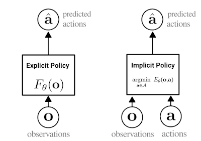Depiction of the difference between explicit (left) and implicit (right) policies. In the implicit policy, the “argmin” means the action that, when paired with a particular observation, minimizes the value of the energy function.

To train Implicit BC models, we use an InfoNCE loss, which trains the network to output low energy for expert actions in the dataset, and high energy for all others (see below). It is interesting to note that this idea of using models that take in both observations and actions is common in reinforcement learning, but not so in supervised policy learning.

Animation of how implicit models can fit discontinuities — in this case, training an implicit model to fit a step (Heaviside) function. Left: 2D plot fitting the black (X) training points — the colors represent the values of the energies (blue is low, brown is high). Middle: 3D plot of the energy model during training. Right: Training loss curve.

Once trained, we find that implicit models are particularly good at precisely modeling discontinuities (above) on which prior explicit models struggle (as in the first figure of this post), resulting in policies that are newly capable of switching decisively between different behaviors.

But why do conventional explicit models struggle? Modern neural networks almost always use continuous activation functions — for example, Tensorflow, Jax, and PyTorch all only ship with continuous activation functions. In attempting to fit discontinuous data, explicit networks built with these activation functions cannot represent discontinuities, so must draw continuous curves between data points. A key aspect of implicit models is that they gain the ability to represent sharp discontinuities, even though the network itself is composed only of continuous layers.

We also establish theoretical foundations for this aspect, specifically a notion of universal approximation. This proves the class of functions that implicit neural networks can represent, which can help justify and guide future research.

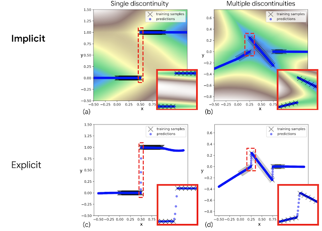Examples of fitting discontinuous functions, for implicit models (top) compared to explicit models (bottom). The red highlighted insets show that implicit models represent discontinuities (a) and (b) while the explicit models must draw continuous lines (c) and (d) in between the discontinuities.

One challenge faced by our initial attempts at this approach was “high action dimensionality”, which means that a robot must decide how to coordinate many motors all at the same time. To scale to high action dimensionality, we use either autoregressive models or Langevin dynamics.

Highlights
In our experiments, we found Implicit BC does particularly well in the real world, including an order of magnitude (10x) better on the 1mm-precision slide-then-insert task compared to a baseline explicit BC model. On this task the implicit model does several consecutive precise adjustments (below) before sliding the block into place. This task demands multiple elements of decisiveness: there are many different possible solutions due to the symmetry of the block and the arbitrary ordering of push maneuvers, and the robot needs to discontinuously decide when the block has been pushed far “enough” before switching to slide it in a different direction. This is in contrast to the indecisiveness that is often associated with continuous-controlled robots.

Example task of sliding a block across a table and precisely inserting it into a slot. These are autonomous behaviors of our Implicit BC policies, using only images (from the shown camera) as input.

A diverse set of different strategies for accomplishing this task. These are autonomous behaviors from our Implicit BC policies, using only images as input.

In another challenging task, the robot needs to sort blocks by color, which presents a large number of possible solutions due to the arbitrary ordering of sorting. On this task the explicit models are customarily indecisive, while implicit models perform considerably better.

Comparison of implicit (left) and explicit (right) BC models on a challenging continuous multi-item sorting task. (4x speed)

In our testing, implicit BC models can also exhibit robust reactive behavior, even when we try to interfere with the robot, despite the model never seeing human hands.

Robust behavior of the implicit BC model despite interfering with the robot.

Overall, we find that Implicit BC policies can achieve strong results compared to state of the art offline reinforcement learning methods across several different task domains. These results include tasks that, challengingly, have either a low number of demonstrations (as few as 19), high observation dimensionality with image-based observations, and/or high action dimensionality up to 30 — which is a large number of actuators to have on a robot.

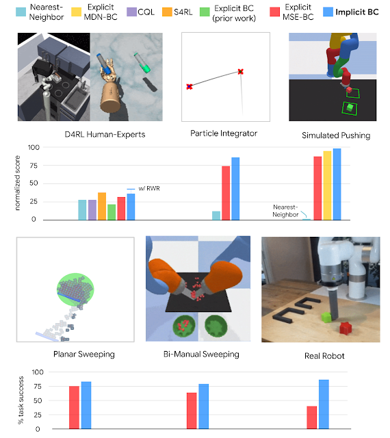Policy learning results of Implicit BC compared to baselines across several domains.

Conclusion
Despite its limitations, behavioral cloning with supervised learning remains one of the simplest ways for robots to learn from examples of human behaviors. As we showed here, replacing explicit policies with implicit policies when doing behavioral cloning allows robots to overcome the "struggle of decisiveness", enabling them to imitate much more complex and precise behaviors. While the focus of our results here was on robot learning, the ability of implicit functions to model sharp discontinuities and multimodal labels may have broader interest in other application domains of machine learning as well.

Acknowledgements
Pete and Corey summarized research performed together with other co-authors: Andy Zeng, Oscar Ramirez, Ayzaan Wahid, Laura Downs, Adrian Wong, Johnny Lee, Igor Mordatch, and Jonathan Tompson. The authors would also like to thank Vikas Sindwhani for project direction advice; Steve Xu, Robert Baruch, Arnab Bose for robot software infrastructure; Jake Varley, Alexa Greenberg for ML infrastructure; and Kamyar Ghasemipour, Jon Barron, Eric Jang, Stephen Tu, Sumeet Singh, Jean-Jacques Slotine, Anirudha Majumdar, Vincent Vanhoucke for helpful feedback and discussions.

Source: Google AI Blog

Permutation-Invariant Neural Networks for Reinforcement Learning

Posted by David Ha, Staff Research Scientist and Yujin Tang, Research Software Engineer, Google Research, Tokyo

“The brain is able to use information coming from the skin as if it were coming from the eyes. We don’t see with the eyes or hear with the ears, these are just the receptors, seeing and hearing in fact goes on in the brain.”

— Paul Bach-y-Rita ¹

People have the amazing ability to use one sensory modality (e.g., touch) to supply environmental information normally gathered by another sense (e.g., vision). This adaptive ability, called sensory substitution, is a phenomenon well-known to neuroscience. While difficult adaptations — such as adjusting to seeing things upside-down, learning to ride a “backwards” bicycle, or learning to “see” by interpreting visual information emitted from a grid of electrodes placed on one’s tongue — require anywhere from weeks, months or even years to attain mastery, people are able to eventually adjust to sensory substitutions.

Examples of Sensory Substitution. Left: Tongue Display Unit (Maris and Bach-y-Rita, 2001; Image: Kaczmarek, 2011). Right: “Upside down goggles” initially conceived by Erismann and Kohler in 1931. (Image Wikipedia).

In contrast, most neural networks are not able to adapt to sensory substitutions at all. For instance, most reinforcement learning (RL) agents require their inputs to be in a pre-specified format, or else they will fail. They expect fixed-size inputs and assume that each element of the input carries a precise meaning, such as the pixel intensity at a specified location, or state information, like position or velocity. In popular RL benchmark tasks (e.g., Ant or Cart-pole), an agent trained using current RL algorithms will fail if its sensory inputs are changed or if the agent is fed additional noisy inputs that are unrelated to the task at hand.

In “The Sensory Neuron as a Transformer: Permutation-Invariant Neural Networks for Reinforcement Learning”, a spotlight paper at NeurIPS 2021, we explore permutation invariant neural network agents, which require each of their sensory neurons (receptors that receive sensory inputs from the environment) to figure out the meaning and context of its input signal, rather than explicitly assuming a fixed meaning. Our experiments show that such agents are robust to observations that contain additional redundant or noisy information, and to observations that are corrupt and incomplete.

Permutation invariant reinforcement learning agents adapting to sensory substitutions. Left: The ordering of the ant’s 28 observations are randomly shuffled every 200 time-steps. Unlike the standard policy, our policy is not affected by the suddenly permuted inputs. Right: Cart-pole agent given many redundant noisy inputs (Interactive web-demo).

In addition to adapting to sensory substitutions in state-observation environments (like the ant and cart-pole examples), we show that these agents can also adapt to sensory substitutions in complex visual-observation environments (such as a CarRacing game that uses only pixel observations) and can perform when the stream of input images is constantly being reshuffled:

We partition the visual input from CarRacing into a 2D grid of small patches, and shuffled their ordering. Without any additional training, our agent still performs even when the original training background (left) is replaced with new images (right).

Method
Our approach takes observations from the environment at each time-step and feeds each element of the observation into distinct, but identical neural networks (called “sensory neurons”), each with no fixed relationship with one another. Each sensory neuron integrates over time information from only their particular sensory input channel. Because each sensory neuron receives only a small part of the full picture, they need to self-organize through communication in order for a global coherent behavior to emerge.

Illustration of observation segmentation.We segment each input into elements, which are then fed to independent sensory neurons. For non-vision tasks where the inputs are usually 1D vectors, each element is a scalar. For vision tasks, we crop each input image into non-overlapping patches.

We encourage neurons to communicate with each other by training them to broadcast messages. While receiving information locally, each individual sensory neuron also continually broadcasts an output message at each time-step. These messages are consolidated and combined into an output vector, called the global latent code, using an attention mechanism similar to that applied in the Transformer architecture. A policy network then uses the global latent code to produce the action that the agent will use to interact with the environment. This action is also fed back into each sensory neuron in the next time-step, closing the communication loop.

Overview of the permutation-invariant RL method. We first feed each individual observation (o_t) into a particular sensory neuron (along with the agent’s previous action, a_t-1). Each neuron then produces and broadcasts a message independently, and an attention mechanism summarizes them into a global latent code (m_t) that is given to the agent's downstream policy network (?) to produce the agent’s action a_t.

Why is this system permutation invariant? Each sensory neuron is an identical neural network that is not confined to only process information from one particular sensory input. In fact, in our setup, the inputs to each sensory neuron are not defined. Instead, each neuron must figure out the meaning of its input signal by paying attention to the inputs received by the other sensory neurons, rather than explicitly assuming a fixed meaning. This encourages the agent to process the entire input as an unordered set, making the system to be permutation invariant to its input. Furthermore, in principle, the agent can use as many sensory neurons as required, thus enabling it to process observations of arbitrary length. Both of these properties will help the agent adapt to sensory substitutions.

Results
We demonstrate the robustness and flexibility of this approach in simpler, state-observation environments, where the observations the agent receives as inputs are low-dimensional vectors holding information about the agent’s states, such as the position or velocity of its components. The agent in the popular Ant locomotion task has a total of 28 inputs with information that includes positions and velocities. We shuffle the order of the input vector several times during a trial and show that the agent is rapidly able to adapt and is still able to walk forward.

In cart-pole, the agent’s goal is to swing up a cart-pole mounted at the center of the cart and balance it upright. Normally the agent sees only five inputs, but we modify the cartpole environment to provide 15 shuffled input signals, 10 of which are pure noise, and the remainder of which are the actual observations from the environment. The agent is still able to perform the task, demonstrating the system’s capacity to work with a large number of inputs and attend only to channels it deems useful. Such flexibility may find useful applications for processing a large unspecified number of signals, most of which are noise, from ill-defined systems.

We also apply this approach to high-dimensional vision-based environments where the observation is a stream of pixel images. Here, we investigate screen-shuffled versions of vision-based RL environments, where each observation frame is divided into a grid of patches, and like a puzzle, the agent must process the patches in a shuffled order to determine a course of action to take. To demonstrate our approach on vision-based tasks, we created a shuffled version of Atari Pong.

Shuffled Pong results. Left: Pong agent trained to play using only 30% of the patches matches performance of Atari opponent. Right: Without extra training, when we give the agent more puzzle pieces, its performance increases.

Here the agent’s input is a variable-length list of patches, so unlike typical RL agents, the agent only gets to “see” a subset of patches from the screen. In the puzzle pong experiment, we pass to the agent a random sample of patches across the screen, which are then fixed through the remainder of the game. We find that we can discard 70% of the patches (at these fixed-random locations) and still train the agent to perform well against the built-in Atari opponent. Interestingly, if we then reveal additional information to the agent (e.g., allowing it access to more image patches), its performance increases, even without additional training. When the agent receives all the patches, in shuffled order, it wins 100% of the time, achieving the same result with agents that are trained while seeing the entire screen.

We find that imposing additional difficulty during training by using unordered observations has additional benefits, such as improving generalization to unseen variations of the task, like when the background of the CarRacing training environment is replaced with a novel image.

Shuffled CarRacing results. The agent has learned to focus its attention (indicated by the highlighted patches) on the road boundaries. Left: Training environment. Right: Test environment with new background.

Conclusion
The permutation invariant neural network agents presented here can handle ill-defined, varying observation spaces. Our agents are robust to observations that contain redundant or noisy information, or observations that are corrupt and incomplete. We believe that permutation invariant systems open up numerous possibilities in reinforcement learning.

If you’re interested to learn more about this work, we invite readers to read our interactive article (pdf version) or watch our video. We also released code to reproduce our experiments.

¹Quoted in Livewired, by David Eagleman. ^↩

Source: Google AI Blog

MetNet-2: Deep Learning for 12-Hour Precipitation Forecasting

Posted by Nal Kalchbrenner and Lasse Espeholt, Google Research

Deep learning has successfully been applied to a wide range of important challenges, such as cancer prevention and increasing accessibility. The application of deep learning models to weather forecasts can be relevant to people on a day-to-day basis, from helping people plan their day to managing food production, transportation systems, or the energy grid. Weather forecasts typically rely on traditional physics-based techniques powered by the world’s largest supercomputers. Such methods are constrained by high computational requirements and are sensitive to approximations of the physical laws on which they are based.

Deep learning offers a new approach to computing forecasts. Rather than incorporating explicit physical laws, deep learning models learn to predict weather patterns directly from observed data and are able to compute predictions faster than physics-based techniques. These approaches also have the potential to increase the frequency, scope, and accuracy of the predicted forecasts.

Illustration of the computation through MetNet-2. As the computation progresses, the network processes an ever larger context from the input and makes a probabilistic forecast of the likely future weather conditions.

Within weather forecasting, deep learning techniques have shown particular promise for nowcasting — i.e., predicting weather up to 2-6 hours ahead. Previous work has focused on using direct neural network models for weather data, extending neural forecasts from 0 to 8 hours with the MetNet architecture, generating continuations of radar data for up to 90 minutes ahead, and interpreting the weather information learned by these neural networks. Still, there is an opportunity for deep learning to extend improvements to longer-range forecasts.

To that end, in “Skillful Twelve Hour Precipitation Forecasts Using Large Context Neural Networks”, we push the forecasting boundaries of our neural precipitation model to 12 hour predictions while keeping a spatial resolution of 1 km and a time resolution of 2 minutes. By quadrupling the input context, adopting a richer weather input state, and extending the architecture to capture longer-range spatial dependencies, MetNet-2 substantially improves on the performance of its predecessor, MetNet. Compared to physics-based models, MetNet-2 outperforms the state-of-the-art HREF ensemble model for weather forecasts up to 12 hours ahead.

MetNet-2 Features and Architecture
Neural weather models like MetNet-2 map observations of the Earth to the probability of weather events, such as the likelihood of rain over a city in the afternoon, of wind gusts reaching 20 knots, or of a sunny day ahead. End-to-end deep learning has the potential to both streamline and increase quality by directly connecting a system's inputs and outputs. With this in mind, MetNet-2 aims to minimize both the complexity and the total number of steps involved in creating a forecast.

The inputs to MetNet-2 include the radar and satellite images also used in MetNet. To capture a more comprehensive snapshot of the atmosphere with information such as temperature, humidity, and wind direction — critical for longer forecasts of up to 12 hours — MetNet-2 also uses the pre-processed starting state used in physical models as a proxy for this additional weather information. The radar-based measures of precipitation (MRMS) serve as the ground truth (i.e., what we are trying to predict) that we use in training to optimize MetNet-2’s parameters.

Example ground truth image: Instantaneous precipitation (mm/hr) based on radar (MRMS) capturing a 12 hours-long progression.

MetNet-2’s probabilistic forecasts can be viewed as averaging all possible future weather conditions weighted by how likely they are. Due to its probabilistic nature, MetNet-2 can be likened to physics-based ensemble models, which average some number of future weather conditions predicted by a variety of physics-based models. One notable difference between these two approaches is the duration of the core part of the computation: ensemble models take ~1 hour, whereas MetNet-2 takes ~1 second.

Steps in a MetNet-2 forecast and in a physics-based ensemble.

One of the main challenges that MetNet-2 must overcome to make 12 hour long forecasts is capturing a sufficient amount of spatial context in the input images. For each additional forecast hour we include 64 km of context in every direction at the input. This results in an input context of size 2048² km² — four times that used in MetNet. In order to process such a large context, MetNet-2 employs model parallelism whereby the model is distributed across 128 cores of a Cloud TPU v3-128. Due to the size of the input context, MetNet-2 replaces the attentional layers of MetNet with computationally more efficient convolutional layers. But standard convolutional layers have local receptive fields that may fail to capture large spatial contexts, so MetNet-2 uses dilated receptive fields, whose size doubles layer after layer, in order to connect points in the input that are far apart one from the other.

Example of input spatial context and target area for MetNet-2.

Results
Because MetNet-2’s predictions are probabilistic, the model’s output is naturally compared with the output of similarly probabilistic ensemble or post-processing models. HREF is one such state-of-the-art ensemble model for precipitation in the United States, which aggregates ten predictions from five different models, twice a day. We evaluate the forecasts using established metrics, such as the Continuous Ranked Probability Score, which captures the magnitude of the probabilistic error of a model’s forecasts relative to the ground truth observations. Despite not performing any physics-based calculations, MetNet-2 is able to outperform HREF up to 12 hours into the future for both low and high levels of precipitation.

Continuous Ranked Probability Score (CRPS; lower is better) for MetNet-2 vs HREF aggregated over a large number of test patches randomly located in the Continental United States.

Examples of Forecasts
The following figures provide a selection of forecasts from MetNet-2 compared with the physics-based ensemble HREF and the ground truth MRMS.

Probability maps for the cumulative precipitation rate of 1 mm/hr on January 3, 2019 over the Pacific NorthWest. The maps are shown for each hour of lead time from 1 to 12. Left: Ground truth, source MRMS. Center: Probability map as predicted by MetNet-2 . Right: Probability map as predicted by HREF.

Comparison of 0.2 mm/hr precipitation on March 30, 2020 over Denver, Colorado. Left: Ground truth, source MRMS. Center: Probability map as predicted by MetNet-2 . Right: Probability map as predicted by HREF.MetNet-2 is able to predict the onset of the storm (called convective initiation) earlier in the forecast than HREF as well as the storm’s starting location, whereas HREF misses the initiation location, but captures its growth phase well.

Comparison of 2 mm/hr precipitation stemming from Hurricane Isaias, an extreme weather event that occurred on August 4, 2020 over the North East coast of the US. Left: Ground truth, source MRMS. Center: Probability map as predicted by MetNet-2. Right: Probability map as predicted by HREF.

Interpreting What MetNet-2 Learns About Weather
Because MetNet-2 does not use hand-crafted physical equations, its performance inspires a natural question: What kind of physical relations about the weather does it learn from the data during training? Using advanced interpretability tools, we further trace the impact of various input features on MetNet-2’s performance at different forecast timelines. Perhaps the most surprising finding is that MetNet-2 appears to emulate the physics described by Quasi-Geostrophic Theory, which is used as an effective approximation of large-scale weather phenomena. MetNet-2 was able to pick up on changes in the atmospheric forces, at the scale of a typical high- or low-pressure system (i.e., the synoptic scale), that bring about favorable conditions for precipitation, a key tenet of the theory.

Conclusion
MetNet-2 represents a step toward enabling a new modeling paradigm for weather forecasting that does not rely on hand-coding the physics of weather phenomena, but rather embraces end-to-end learning from observations to weather targets and parallel forecasting on low-precision hardware. Yet many challenges remain on the path to fully achieving this goal, including incorporating more raw data about the atmosphere directly (rather than using the pre-processed starting state from physical models), broadening the set of weather phenomena, increasing the lead time horizon to days and weeks, and widening the geographic coverage beyond the United States.

Acknowledgements
Shreya Agrawal, Casper Sønderby, Manoj Kumar, Jonathan Heek, Carla Bromberg, Cenk Gazen, Jason Hickey, Aaron Bell, Marcin Andrychowicz, Amy McGovern, Rob Carver, Stephan Hoyer, Zack Ontiveros, Lak Lakshmanan, David McPeek, Ian Gonzalez, Claudio Martella, Samier Merchant, Fred Zyda, Daniel Furrer and Tom Small.

Source: Google AI Blog

Making Better Future Predictions by Watching Unlabeled Videos

Posted by Dave Epstein, Student Researcher and Chen Sun, Staff Research Scientist, Google Research

Machine learning (ML) agents are increasingly deployed in the real world to make decisions and assist people in their daily lives. Making reasonable predictions about the future at varying timescales is one of the most important capabilities for such agents because it enables them to predict changes in the world around them, including other agents’ behaviors, and plan how to act next. Importantly, successful future prediction requires both capturing meaningful transitions in the environment (e.g., dough transforming into bread) and adapting to how transitions unfold over time in order to make decisions.

Previous work in future prediction from visual observations has largely been constrained by the format of its output (e.g., pixels that represent an image) or a manually-defined set of human activities (e.g., predicting if someone will keep walking, sit down, or jump). These are either too detailed and hard to predict or lack important information about the richness of the real world. For example, predicting “person jumping” does not capture why they’re jumping, what they’re jumping onto, etc. Also, with very few exceptions, previous models were designed to make predictions at a fixed offset into the future, which is a limiting assumption because we rarely know when meaningful future states will happen.

For example, in a video about making ice cream (depicted below), the meaningful transition from “cream” to “ice cream” occurs over 35 seconds, so models predicting such transitions would need to look 35 seconds ahead. But this time interval varies a large amount across different activities and videos — meaningful transitions occur at any distance into the future. Learning to make such predictions at flexible intervals is hard because the desired ground truth may be relatively ambiguous. For example, the correct prediction could be the just-churned ice cream in the machine, or scoops of the ice cream in a bowl. In addition, collecting such annotations at scale (i.e., frame-by-frame for millions of videos) is infeasible. However, many existing instructional videos come with speech transcripts, which often offer concise, general descriptions throughout entire videos. This source of data can guide a model’s attention toward important parts of the video, obviating the need for manual labeling and allowing a flexible, data-driven definition of the future.

In “Learning Temporal Dynamics from Cycles in Narrated Video”, published at ICCV 2021, we propose an approach that is self-supervised, using a recent large unlabeled dataset of diverse human action. The resulting model operates at a high level of abstraction, can make predictions arbitrarily far into the future, and chooses how far into the future to predict based on context. Called Multi-Modal Cycle Consistency (MMCC), it leverages narrated instructional video to learn a strong predictive model of the future. We demonstrate how MMCC can be applied, without fine-tuning, to a variety of challenging tasks, and qualitatively examine its predictions. In the example below, MMCC predicts the future (d) from present frame (a), rather than less relevant potential futures (b) or (c).

This work uses cues from vision and language to predict high-level changes (such as cream becoming ice cream) in video (video from HowTo100M).

Viewing Videos as Graphs
The foundation of our method is to represent narrated videos as graphs. We view videos as a collection of nodes, where nodes are either video frames (sampled at 1 frame per second) or segments of narrated text (extracted with automatic speech recognition systems), encoded by neural networks. During training, MMCC constructs a graph from the nodes, using cross-modal edges to connect video frames and text segments that refer to the same state, and temporal edges to connect the present (e.g., strawberry-flavored cream) and the future (e.g., soft-serve ice cream). The temporal edges operate on both modalities equally — they can start from either a video frame, some text, or both, and can connect to a future (or past) state in either modality. MMCC achieves this by learning a latent representation shared by frames and text and then making predictions in this representation space.

Multi-modal Cycle Consistency
To learn the cross-modal and temporal edge functions without supervision, we apply the idea of cycle consistency. Here, cycle consistency refers to the construction of cycle graphs, in which the model constructs a series of edges from an initial node to other nodes and back again: Given a start node (e.g., a sample video frame), the model is expected to find its cross-modal counterpart (i.e., text describing the frame) and combine them as the present state. To do this, at the start of training, the model assumes that frames and text with the same timestamps are counterparts, but then relaxes this assumption later. The model then predicts a future state, and the node most similar to this prediction is selected. Finally, the model attempts to invert the above steps by predicting the present state backward from the future node, and thus connecting the future node back with the start node.

The discrepancy between the model’s prediction of the present from the future and the actual present is the cycle-consistency loss. Intuitively, this training objective requires the predicted future to contain enough information about its past to be invertible, leading to predictions that correspond to meaningful changes to the same entities (e.g., tomato becoming marinara sauce, or flour and eggs in a bowl becoming dough). Moreover, the inclusion of cross-modal edges ensures future predictions are meaningful in either modality.

To learn the temporal and cross-modal edge functions end-to-end, we use the soft attention technique, which first outputs how likely each node is to be the target node of the edge, and then “picks” a node by taking the weighted average among all possible candidates. Importantly, this cyclic graph constraint makes few assumptions for the kind of temporal edges the model should learn, as long as they end up forming a consistent cycle. This enables the emergence of long-term temporal dynamics critical for future prediction without requiring manual labels of meaningful changes.

An example of the training objective: A cycle graph is expected to be constructed between the chicken with soy sauce and the chicken in chili oil because they are two adjacent steps in the chicken’s preparation (video from HowTo100M).

Discovering Cycles in Real-World Video
MMCC is trained without any explicit ground truth, using only long video sequences and randomly sampled starting conditions (a frame or text excerpt) and asking the model to find temporal cycles. After training, MMCC can identify meaningful cycles that capture complex changes in video.

Given frames as input (left), MMCC selects relevant text from video narrations and uses both modalities to predict a future frame (middle). It then finds text relevant to this future and uses it to predict the past (right). Using its knowledge of how objects and scenes change over time, MMCC “closes the cycle” and ends up where it started (videos from HowTo100M).

The model can also start from narrated text rather than frames and still find relevant transitions (videos from HowTo100M).

Zero-Shot Applications
For MMCC to identify meaningful transitions over time in an entire video, we define a “likely transition score” for each pair (A, B) of frames in a video, according to the model's predictions — the closer B is to our model’s prediction of the future of A, the higher the score assigned. We then rank all pairs according to this score and show the highest-scoring pairs of present and future frames detected in previously unseen videos (examples below).

The highest-scoring pairs from eight random videos, which showcase the versatility of the model across a wide range of tasks (videos from HowTo100M).

We can use this same approach to temporally sort an unordered collection of video frames without any fine-tuning by finding an ordering that maximizes the overall confidence scores between all adjacent frames in the sorted sequence.

Left: Shuffled frames from three videos. Right: MMCC unshuffles the frames. The true order is shown under each frame. Even when MMCC does not predict the ground truth, its predictions often appear reasonable, and so, it can present an alternate ordering (videos from HowTo100M).

Evaluating Future Prediction
We evaluate the model’s ability to anticipate action, potentially minutes in advance, using the top-k recall metric, which here measures a model’s ability to retrieve the correct future (higher is better). On CrossTask, a dataset of instruction videos with labels describing key steps, MMCC outperforms the previous self-supervised state-of-the-art models in inferring possible future actions.

	Recall
Model	Top-1	Top-5	Top-10
Cross-modal	2.9	14.2	24.3
Repr. Ant.	3.0	13.3	26.0
MemDPC	2.9	15.8	27.4
TAP	4.5	17.1	27.9
MMCC	5.4	19.9	33.8

Conclusions
We have introduced a self-supervised method to learn temporal dynamics by cycling through narrated instructional videos. Despite the simplicity of the model’s architecture, it can discover meaningful long-term transitions in vision and language, and can be applied without further training to challenging downstream tasks, such as anticipating far-away action and ordering collections of images. An interesting future direction is transferring the model to agents so they can use it to conduct long-term planning.

Acknowledgements
The core team includes Dave Epstein, Jiajun Wu, Cordelia Schmid, and Chen Sun. We thank Alexei Efros, Mia Chiquier, and Shiry Ginosar for their feedback, and Allan Jabri for inspiration in figure design. Dave would like to thank Dídac Surís and Carl Vondrick for insightful early discussions on cycling through time in video.

Source: Google AI Blog

Machine Learning Communities: Q3 ‘21 highlights and achievements

Posted by HyeJung Lee, DevRel Community Manager and Soonson Kwon, DevRel Program Manager

Let’s explore highlights and achievements of vast Google Machine Learning communities by region for the last quarter. Activities of experts (GDE, professional individuals), communities (TFUG, TensorFlow user groups), students (GDSC, student clubs), and developers groups (GDG) are presented here.

Key highlights

Image shows a banner for 30 days of ML with Kaggle

30 days of ML with Kaggle is designed to help beginners study ML using Kaggle Learn courses as well as a competition specifically for the participants of this program. Collaborated with the Kaggle team so that +30 the ML GDEs and TFUG organizers participated as volunteers as online mentors as well as speakers for this initiative.

Total 16 of the GDE/GDSC/TFUGs run community organized programs by referring to the shared community organize guide. Houston TensorFlow & Applied AI/ML placed 6th out of 7573 teams — the only Americans in the Top 10 in the competition. And TFUG Santiago (Chile) organizers participated as well and they are number 17 on the public leaderboard.

Asia Pacific

Image shows Google Cloud and Coca-Cola logos

GDE Minori MATSUDA (Japan)’s project on Coca-Cola Bottlers Japan was published on Google Cloud Japan Blog covering creating an ML pipeline to deploy into real business within 2 months by using Vertex AI. This is also published on GCP blog in English.

GDE Chansung Park (Korea) and Sayak Paul (India) published many articles on GCP Blog. First, “Image search with natural language queries” explained how to build a simple image parser from natural language inputs using OpenAI's CLIP model. From this second “Model training as a CI/CD system: (Part I, Part II)” post, you can learn more about why having a resilient CI/CD system for your ML application is crucial for success. Last, “Dual deployments on Vertex AI” talks about end-to-end workflow using Vertex AI, TFX and Kubeflow.

In China, GDE Junpeng Ye used TensorFlow 2.x to significantly reduce the codebase (15k → 2k) on WeChat Finder which is a TikTok alternative in WeChat. GDE Dan lee wrote an article on Understanding TensorFlow Series: Part 1, Part 2, Part 3-1, Part 3-2, Part 4

GDE Ngoc Ba from Vietnam has contributed AI Papers Reading and Coding series implementing ML/DL papers in TensorFlow and creates slides/videos every two weeks. (videos: Vit Transformer, MLP-Mixer and Transformer)

A beginner friendly codelabs (Get started with audio classification ,Go further with audio classification) by GDSC Sookmyung (Korea) learning to customize pre-trained audio classification models to your needs and deploy them to your apps, using TFlite Model Maker.

Cover image for Mat Kelcey's talk on JAX at the PyConAU event

GDE Matthew Kelcey from Australia gave a talk on JAX at PyConAU event. Mat gave an overview to fundamentals of JAX and an intro to some of the libraries being developed on top.

Image shows overview for the released PerceiverIO code

In Singapore, TFUG Singapore dived back into some of the latest papers, techniques, and fields of research that are delivering state-of-the-art results in a number of fields. GDE Martin Andrews included a brief code walkthrough for the released PerceiverIO code at perceiver- highlighting what JAX looks like, how Haiku relates to Sonnet, but also the data loading stuff which is done via tf.data.

Machine Learning Experimentation with TensorBoard book cover

GDE Imran us Salam Mian from Pakistan published a book "Machine Learning Experimentation with TensorBoard".

India

GDE Aakash Nain has published the TF-JAX tutorial series from Part 4 to Part 8. Part 4 gives a brief introduction about JAX (What/Why), and DeviceArray. Part 5 covers why pure functions are good and why JAX prefers them. Part 6 focuses on Pseudo Random Number Generation (PRNG) in Numpy and JAX. Part 7 focuses on Just In Time Compilation (JIT) in JAX. And Part 8 covers vmap and pmap.

Image of Bhavesh's Google Cloud certificate

GDE Bhavesh Bhatt published a video about his experience on the Google Cloud Professional Data Engineer certification exam.

Image shows phase 1 and 2 of the Climate Change project using Vertex AI

Climate Change project using Vertex AI by ML GDE Sayak Paul and Siddha Ganju (NVIDIA). They published a paper (Flood Segmentation on Sentinel-1 SAR Imagery with Semi-Supervised Learning) and open-sourced the project with regard to NASA Impact's ETCI competition. This project made four NeurIPS workshops AI for Science: Mind the Gaps, Tackling Climate Change with Machine Learning, Women in ML, and Machine Learning and the Physical Sciences. And they finished as the first runners-up (see Test Phase 2).

Image shows example of handwriting recognition tutorial

Tutorial on handwriting recognition was contributed to Keras example by GDE Sayak Paul and Aakash Kumar Nain.

Graph regularization for image classification using synthesized graphs by GDE Sayak Pau was added to the official examples in the Neural Structured Learning in TensorFlow.

GDE Sayak Paul and Soumik Rakshit shared a new NLP dataset for multi-label text classification. The dataset consists of paper titles, abstracts, and term categories scraped from arXiv.

North America

Banner image shows students participating in Google Summer of Code

During the GSoC (Google Summer of Code), some GDEs mentored or co-mentored students. GDE Margaret Maynard-Reid (USA) mentored TF-GAN, Model Garden, TF Hub and TFLite products. You can get some of her experience and tips from the GDE Blog. And you can find GDE Sayak Paul (India) and Googler Morgan Roff’s GSoC experience in (co-)mentoring TensorFlow and TF Hub as well.

A beginner friendly workshop on TensorFlow with ML GDE Henry Ruiz (USA) was hosted by GDSC Texas A&M University (USA) for the students.

Screenshot from Youtube video on how transformers work

Youtube video Self-Attention Explained: How do Transformers work? by GDE Tanmay Bakshi from Canada explained how you can build a Transformer encoder-based neural network to classify code into 8 different programming languages using TPU, Colab with Keras.

Europe

GDG / GDSC Turkey hosted AI Summer Camp in cooperation with Global AI Hub. 7100 participants learned about ML, TensorFlow, CV and NLP.

Screenshot from slide presentation titled Why Jax?

TechTalk Speech Processing with Deep Learning and JAX/Trax by GDE Sergii Khomenko (Germany) and M. Yusuf Sarıgöz (Turkey). They reviewed technologies such as Jax, TensorFlow, Trax, and others that can help boost our research in speech processing.

South/Central America

Image shows Custom object detection in the browser using TensorFlow.js

On the other side of the world, in Brazil, GDE Hugo Zanini Gomes wrote an article about “Custom object detection in the browser using TensorFlow.js” using the TensorFlow 2 Object Detection API and Colab was posted on the TensorFlow blog.

Screenshot from a talk about Real-time semantic segmentation in the browser - Made with TensorFlow.js

And Hugo gave a talk about Real-time semantic segmentation in the browser - Made with TensorFlow.js covered using SavedModels in an efficient way in JavaScript directly enabling you to get the reach and scale of the web for your new research.

Data Pipelines for ML was talked about by GDE Nathaly Alarcon Torrico from Bolivia explained all the phases involved in the creation of ML and Data Science products, starting with the data collection, transformation, storage and Product creation of ML models.

Screensho from TechTalk “Machine Learning Competitivo: Top 1% en Kaggle (Video)

TechTalk “Machine Learning Competitivo: Top 1% en Kaggle (Video)“ was hosted by TFUG Santiago (Chile). In this talk the speaker gave a tour of the steps to follow to generate a model capable of being in the top 1% of the Kaggle Leaderboard. The focus was on showing the libraries and“ tricks ”that are used to be able to test many ideas quickly both in implementation and in execution and how to use them in productive environments.

MENA

Screenshot from workshop about Recurrent Neural Networks

GDE Ruqiya Bin Safi (Saudi Arabia) had a workshop about Recurrent Neural Networks : part 1 (Github / Slide) at the GDG Mena. And Ruqiya gave a talk about Recurrent Neural Networks: part 2 at the GDG Cloud Saudi (Saudi Arabia).

AI Training with Kaggle by GDSC Islamic University of Gaza from Palestine. It is a two month training covering Data Processing, Image Processing and NLP with Kaggle.

Sub-Saharan Africa

TFUG Ibadan had two TensorFlow events : Basic Sentiment analysis with Tensorflow and Introduction to Recommenders Systems with TensorFlow”.

Image of Yannick Serge Obam Akou's TensorFlow Certificate

Article covered some tips to study, prepare and pass the TensorFlow developer exam in French by ML GDE Yannick Serge Obam Akou (Cameroon).

Source: Google Developers Blog

Practical Differentially Private Clustering

Posted by Alisa Chang, Software Engineer, Google Cloud and Pritish Kamath, Research Scientist, Google Research

Over the last several years, progress has been made on privacy-safe approaches for handling sensitive data, for example, while discovering insights into human mobility and through use of federated analytics such as RAPPOR. In 2019, we released an open source library to enable developers and organizations to use techniques that provide differential privacy, a strong and widely accepted mathematical notion of privacy. Differentially-private data analysis is a principled approach that enables organizations to learn and release insights from the bulk of their data while simultaneously providing a mathematical guarantee that those results do not allow any individual user's data to be distinguished or re-identified.

In this post, we consider the following basic problem: Given a database containing several attributes about users, how can one create meaningful user groups and understand their characteristics? Importantly, if the database at hand contains sensitive user attributes, how can one reveal these group characteristics without compromising the privacy of individual users?

Such a task falls under the broad umbrella of clustering, a fundamental building block in unsupervised machine learning. A clustering method partitions the data points into groups and provides a way to assign any new data point to a group with which it is most similar. The k-means clustering algorithm has been one such influential clustering method. However, when working with sensitive datasets, it can potentially reveal significant information about individual data points, putting the privacy of the corresponding user at risk.

Today, we announce the addition of a new differentially private clustering algorithm to our differential privacy library, which is based on privately generating new representative data points. We evaluate its performance on multiple datasets and compare to existing baselines, finding competitive or better performance.

K-means Clustering
Given a set of data points, the goal of k-means clustering is to identify (at most) k points, called cluster centers, so as to minimize the loss given by the sum of squared distances of the data points from their closest cluster center. This partitions the set of data points into k groups. Moreover, any new data point can be assigned to a group based on its closest cluster center. However, releasing the set of cluster centers has the potential to leak information about particular users — for example, consider a scenario where a particular data point is significantly far from the rest of the points, so the standard k-means clustering algorithm returns a cluster center at this single point, thereby revealing sensitive information about this single point. To address this, we design a new algorithm for clustering with the k-means objective within the framework of differential privacy.

A Differentially Private Algorithm
In “Locally Private k-Means in One Round”, published at ICML 2021, we presented a differentially private algorithm for clustering data points. That algorithm had the advantage of being private in the local model, where the user’s privacy is protected even from the central server performing the clustering. However, any such approach necessarily incurs a significantly larger loss than approaches using models of privacy that require trusting a central server.¹

Here, we present a similarly inspired clustering algorithm that works in the central model of differential privacy, where the central server is trusted to have complete access to the raw data, and the goal is to compute differentially private cluster centers, which do not leak information about individual data points. The central model is the standard model for differential privacy, and algorithms in the central model can be more easily substituted in place of their non-private counterparts since they do not require changes to the data collection process. The algorithm proceeds by first generating, in a differentially private manner, a core-set that consists of weighted points that “represent” the data points well. This is followed by executing any (non-private) clustering algorithm (e.g., k-means++) on this privately generated core-set.

At a high level, the algorithm generates the private core-set by first using random-projection–based locality-sensitive hashing (LSH) in a recursive manner² to partition the points into “buckets” of similar points, and then replacing each bucket by a single weighted point that is the average of the points in the bucket, with a weight equal to the number of points in the same bucket. As described so far, though, this algorithm is not private. We make it private by performing each operation in a private manner by adding noise to both the counts and averages of points within a bucket.

This algorithm satisfies differential privacy because each point’s contributions to the bucket counts and the bucket averages are masked by the added noise, so the behavior of the algorithm does not reveal information about any individual point. There is a tradeoff with this approach: if the number of points in the buckets is too large, then individual points will not be well-represented by points in the core-set, whereas if the number of points in a bucket is too small, then the added noise (to the counts and averages) will become significant in comparison to the actual values, leading to poor quality of the core-set. This trade-off is realized with user-provided parameters in the algorithm that control the number of points that can be in a bucket.

Visual illustration of the algorithm.

Experimental Evaluation
We evaluated the algorithm on a few benchmark datasets, comparing its performance to that of the (non-private) k-means++ algorithm, as well as a few other algorithms with available implementations, namely diffprivlib and dp-clustering-icml17. We use the following benchmark datasets: (i) a synthetic dataset consisting of 100,000 data points in 100 dimensions sampled from a mixture of 64 Gaussians; (ii) neural representations for the MNIST dataset on handwritten digits obtained by training a LeNet model; (iii) the UC Irvine dataset on Letter Recognition; and (iv) the UC Irvine dataset on Gas Turbine CO and NOx Emissions.³

We analyze the normalized k-means loss (mean squared distance from data points to the nearest center) while varying the number of target centers (k) for these benchmark datasets.⁴ The described algorithm achieves a lower loss than the other private algorithms in three out of the four datasets we consider.

Normalized loss for varying k = number of target clusters (lower is better). The solid curves denote the mean over the 20 runs, and the shaded region denotes the 25-75^th percentile range.

Moreover, for datasets with specified ground-truth labels (i.e., known groupings), we analyze the cluster label accuracy, which is the accuracy of the labeling obtained by assigning the most frequent ground-truth label in each cluster found by the clustering algorithm to all points in that cluster. Here, the described algorithm performs better than other private algorithms for all the datasets with pre-specified ground-truth labels that we consider.

Cluster label accuracy for varying k = number of target clusters (higher is better). The solid curves denote the mean over the 20 runs, and the shaded region denotes the 25-75^th percentile range.

Limitations and Future Directions
There are a couple of limitations to consider when using this or any other library for private clustering.

It is important to separately account for the privacy loss in any preprocessing (e.g., centering the data points or rescaling the different coordinates) done before using the private clustering algorithm. So, we hope to provide support for differentially private versions of commonly used preprocessing methods in the future and investigate changes so that the algorithm performs better with data that isn’t necessarily preprocessed.
The algorithm described requires a user-provided radius, such that all data points lie within a sphere of that radius. This is used to determine the amount of noise that is added to the bucket averages. Note that this differs from diffprivlib and dp-clustering-icml17 which take in different notions of bounds of the dataset (e.g., a minimum and maximum of each coordinate). For the sake of our experimental evaluation, we calculated the relevant bounds non-privately for each dataset. However, when running the algorithms in practice, these bounds should generally be privately computed or provided without knowledge of the dataset (e.g., using the underlying range of the data). Although, note that in case of the algorithm described, the provided radius need not be exactly correct; any data points outside of the provided radius are replaced with the closest points that are within the sphere of that radius.

Conclusion
This work proposes a new algorithm for computing representative points (cluster centers) within the framework of differential privacy. With the rise in the amount of datasets collected around the world, we hope that our open source tool will help organizations obtain and share meaningful insights about their datasets, with the mathematical assurance of differential privacy.

Acknowledgements
We thank Christoph Dibak, Badih Ghazi, Miguel Guevara, Sasha Kulankhina, Ravi Kumar, Pasin Manurangsi, Jane Shapiro, Daniel Simmons-Marengo, Yurii Sushko, and Mirac Vuslat Basaran for their help.

¹As shown by Uri Stemmer in Locally private k-means clustering (SODA 2020). ^↩
²This is similar to work on LSH Forest, used in the context of similarity-search queries. ^↩
³Datasets (iii) and (iv) were centered to have mean zero before evaluating the algorithms. ^↩
⁴Evaluation done for fixed privacy parameters ε = 1.0 and δ = 1e-6. Note that dp-clustering-icml17 works in the pure differential privacy model (namely, with δ = 0); k-means++, of course, has no privacy parameters. ^↩

Source: Google AI Blog

How Underspecification Presents Challenges for Machine Learning

Posted by Alex D’Amour and Katherine Heller, Research Scientists, Google Research

Machine learning (ML) models are being used more widely today than ever before and are becoming increasingly impactful. However, they often exhibit unexpected behavior when they are used in real-world domains. For example, computer vision models can exhibit surprising sensitivity to irrelevant features, while natural language processing models can depend unpredictably on demographic correlations not directly indicated by the text. Some reasons for these failures are well-known: for example, training ML models on poorly curated data, or training models to solve prediction problems that are structurally mismatched with the application domain. Yet, even when these known problems are handled, model behavior can still be inconsistent in deployment, varying even between training runs.

In “Underspecification Presents Challenges for Credibility in Modern Machine Learning”, to be published in the Journal of Machine Learning Research, we show that a key failure mode especially prevalent in modern ML systems is underspecification. The idea behind underspecification is that while ML models are validated on held-out data, this validation is often insufficient to guarantee that the models will have well-defined behavior when they are used in a new setting. We show that underspecification appears in a wide variety of practical ML systems and suggest some strategies for mitigation.

Underspecification
ML systems have been successful largely because they incorporate validation of the model on held-out data to ensure high performance. However, for a fixed dataset and model architecture, there are often many distinct ways that a trained model can achieve high validation performance. But under standard practice, models that encode distinct solutions are often treated as equivalent because their held-out predictive performance is approximately equivalent.

Importantly, the distinctions between these models do become clear when they are measured on criteria beyond standard predictive performance, such as fairness or robustness to irrelevant input perturbations. For example, among models that perform equally well on standard validations, some may exhibit greater performance disparities between social groups than others, or rely more heavily on irrelevant information. These differences, in turn, can translate to real differences in behavior when the model is used in real-world scenarios.

Underspecification refers to this gap between the requirements that practitioners often have in mind when they build an ML model, and the requirements that are actually enforced by the ML pipeline (i.e., the design and implementation of a model). An important consequence of underspecification is that even if the pipeline could in principle return a model that meets all of these requirements, there is no guarantee that in practice the model will satisfy any requirement beyond accurate prediction on held-out data. In fact, the model that is returned may have properties that instead depend on arbitrary or opaque choices made in the implementation of the ML pipeline, such as those arising from random initialization seeds, data ordering, hardware, etc. Thus, ML pipelines that do not include explicit defects may still return models that behave unexpectedly in real-world settings.

Identifying Underspecification in Real Applications
In this work, we investigated concrete implications of underspecification in the kinds of ML models that are used in real-world applications. Our empirical strategy was to construct sets of models using nearly identical ML pipelines, to which we only applied small changes that had no practical effect on standard validation performance. Here, we focused on the random seed used to initialize training and determine data ordering. If important properties of the model can be substantially influenced by these changes, it indicates that the pipeline does not fully specify this real-world behavior. In every domain where we conducted this experiment, we found that these small changes induced substantial variation on axes that matter in real-world use.

Underspecification in Computer Vision
As an example, consider underspecification and its relationship to robustness in computer vision. A central challenge in computer vision is that deep models often suffer from brittleness under distribution shifts that humans do not find challenging. For instance, image classification models that perform well on the ImageNet benchmark are known to perform poorly on benchmarks like ImageNet-C, which apply common image corruptions, such as pixelization or motion blur, to the standard ImageNet test set.

In our experiment, we showed that model sensitivity to these corruptions is underspecified by standard pipelines. Following the strategy discussed above, we generated fifty ResNet-50 image classification models using the same pipeline and the same data. The only difference between these models was the random seed used in training. When evaluated on the standard ImageNet validation set, these models achieved practically equivalent performance. However, when the models were evaluated on different test sets in the ImageNet-C benchmark (i.e., on corrupted data), performance on some tests varied by orders of magnitude more than on standard validations. This pattern persisted for larger-scale models that were pre-trained on much larger datasets (e.g., a BiT-L model pre-trained on the 300 million image JFT-300M dataset). For these models, varying the random seed at the fine-tuning stage of training produced a similar pattern of variations.

Left: Parallel axis plots showing the variation in accuracy between identical, randomly initialized ResNet-50 models on strongly corrupted ImageNet-C data. Lines represent the performance of each model in the ensemble on classification tasks using uncorrupted test data, as well as corrupted data (pixelation, contrast, motion blur, and brightness). Given values are the deviation in accuracy from the ensemble mean, scaled by the standard deviation of accuracies on the “clean” ImageNet test set. The solid black line highlights the performance of an arbitrarily selected model to show how performance on one test may not be a good indication of performance on others. Right: Example images from the standard ImageNet test set, with corrupted versions from the ImageNet-C benchmark.

We also showed that underspecification can have practical implications in special-purpose computer vision models built for medical imaging, where deep learning models have shown great promise. We considered two research pipelines intended as precursors for medical applications: one ophthalmology pipeline for building models that detect diabetic retinopathy and referable diabetic macular edema from retinal fundus images, and one dermatology pipeline for building models to recognize common dermatological conditions from photographs of skin. In our experiments, we considered pipelines that were validated only on randomly held-out data.

We then stress-tested models produced by these pipelines on practically important dimensions. For the ophthalmology pipeline, we tested how models trained with different random seeds performed when applied to images taken from a new camera type not encountered during training. For the dermatology pipeline, the stress test was similar, but for patients with different estimated skin types (i.e., non-dermatologist evaluation of tone and response to sunlight). In both cases, we found that standard validations were not enough to fully specify the trained model’s performance on these axes. In the ophthalmology application, the random seed used in training induced wider variability in performance on a new camera type than would have been expected from standard validations, and in the dermatology application, the random seed induced similar variation in performance in skin-type subgroups, even though the overall performance of the models was stable across seeds.

These results reiterate that standard hold-out testing alone is not sufficient to ensure acceptable model behavior in medical applications, underscoring the need for expanded testing protocols for ML systems intended for application in the medical domain. In the medical literature, such validations are termed "external validation" and have historically been part of reporting guidelines such as STARD and TRIPOD. These are being emphasized in updates such as STARD-AI and TRIPOD-AI. Finally, as part of regulated medical device development processes (see, e.g., US and EU regulations), there are other forms of safety and performance related considerations, such as mandatory compliance to standards for risk management, human factors engineering, clinical validations and accredited body reviews, that aim to ensure acceptable medical application performance.

Relative variability of medical imaging models on stress tests, using the same conventions as the figure above. Top left: Variation in AUC between diabetic retinopathy classification models trained using different random seeds when evaluated on images from different camera types. In this experiment, camera type 5 was not encountered during training. Bottom left: Variation in accuracy between skin condition classification models trained using different random seeds when evaluated on different estimated skin types (approximated by dermatologist-trained laypersons from retrospective photographs and potentially subject to labeling errors). Right: example images from the original test set (left) and the stress test set (right).

Underspecification in Other Applications

The cases discussed above are a small subset of models that we probed for underspecification. Other cases we examined include:

Natural Language Processing: We showed that on a variety of NLP tasks, underspecification affected how models derived from BERT-processed sentences. For example, depending on the random seed, a pipeline could produce a model that depends more or less on correlations involving gender (e.g., between gender and occupation) when making predictions.
Acute Kidney Injury (AKI) prediction: We showed that underspecification affects reliance on operational versus physiological signals in AKI prediction models based on electronic health records.
Polygenic Risk Scores (PRS): We showed that underspecification influences the ability for (PRS) models, which predict clinical outcomes based on patient genomic data, to generalize across different patient populations.

In each case, we showed that these important properties are left ill-defined by standard training pipelines, making them sensitive to seemingly innocuous choices.

Conclusion
Addressing underspecification is a challenging problem. It requires full specification and testing of requirements for a model beyond standard predictive performance. Doing this well needs full engagement with the context in which the model will be used, an understanding of how the training data were collected, and often, incorporation of domain expertise when the available data fall short. These aspects of ML system design are often underemphasized in ML research today. A key goal of this work is to show how underinvestment in this area can manifest concretely, and to encourage the development of processes for fuller specification and testing of ML pipelines.

Some important first steps in this area are to specify stress testing protocols for any applied ML pipeline that is meant to see real-world use. Once these criteria are codified in measurable metrics, a number of different algorithmic strategies may be useful for improving them, including data augmentation, pretraining, and incorporation of causal structure. It should be noted, however, that ideal stress testing and improvement processes will usually require iteration: both the requirements for ML systems, and the world in which they are used, are constantly changing.

Acknowledgements
We would like to thank all of our co-authors, Dr. Nenad Tomasev (DeepMind), Prof. Finale Doshi-Velez (Harvard SEAS), UK Biobank, and our partners, EyePACS, Aravind Eye Hospital and Sankara Nethralaya.

Source: Google AI Blog

Baselines for Uncertainty and Robustness in Deep Learning

Posted by Zachary Nado, Research Engineer and Dustin Tran, Research Scientist, Google Research, Brain Team

Machine learning (ML) is increasingly being used in real-world applications, so understanding the uncertainty and robustness of a model is necessary to ensure performance in practice. For example, how do models behave when deployed on data that differs from the data on which they were trained? How do models signal when they are likely to make a mistake?

To get a handle on an ML model's behavior, its performance is often measured against a baseline for the task of interest. With each baseline, researchers must try to reproduce results only using descriptions from the corresponding papers , which results in serious challenges for replication. Having access to the code for experiments may be more useful, assuming it is well-documented and maintained. But even this is not enough, because the baselines must be rigorously validated. For example, in retrospective analyses over a collection of works [1, 2, 3], authors often find that a simple well-tuned baseline outperforms more sophisticated methods. In order to truly understand how models perform relative to each other, and enable researchers to measure whether new ideas in fact yield meaningful progress, models of interest must be compared to a common baseline.

In “Uncertainty Baselines: Benchmarks for Uncertainty & Robustness in Deep Learning”, we introduce Uncertainty Baselines, a collection of high-quality implementations of standard and state-of-the-art deep learning methods for a variety of tasks, with the goal of making research on uncertainty and robustness more reproducible. The collection spans 19 methods across nine tasks, each with at least five metrics. Each baseline is a self-contained experiment pipeline with easily reusable and extendable components and with minimal dependencies outside of the framework in which it is written. The included pipelines are implemented in TensorFlow, PyTorch, and Jax. Additionally, the hyperparameters for each baseline have been extensively tuned over numerous iterations so as to provide even stronger results.

Uncertainty Baselines
As of this writing, Uncertainty Baselines provides a total of 83 baselines, comprising 19 methods encompassing standard and more recent strategies over nine datasets. Example methods include BatchEnsemble, Deep Ensembles, Rank-1 Bayesian Neural Nets, Monte Carlo Dropout, and Spectral-normalized Neural Gaussian Processes. It acts as a successor in merging several popular benchmarks in the community: Can You Trust Your Model's Uncertainty?, BDL benchmarks, and Edward2's baselines.

Dataset	Inputs	Output	Train Examples	Test Datasets

CIFAR	RGB images	10-class distribution	50,000	3

ImageNet	RGB images	1000-class distribution	1,281,167	6

CLINC Intent Detection	Dialog system query text	150-class distribution (in 10 domains)	15,000	2

Kaggle's Diabetic Retinopathy Detection	RGB images	Probability of Diabetic Retinopathy	35,126	1

Wikipedia Toxicity	Wikipedia comment text	Probability of toxicity	159,571	3

A subset of 5 out of 9 available datasets for which baselines are provided. The datasets span tabular, text, and image modalities.

Uncertainty Baselines sets up each baseline under a choice of base model, training dataset, and a suite of evaluation metrics. Each is then tuned over its hyperparameters to maximize performance on such metrics. The available baselines vary among these three axes:

Base models (architectures) include Wide ResNet 28-10, ResNet-50, BERT, and simple fully-connected networks.
Training datasets include standard machine learning datasets (CIFAR, ImageNet, and UCI) as well as more real-world problems (Clinc Intent Detection, Kaggle’s Diabetic Retinopathy Detection, and Wikipedia Toxicity).
Evaluation includes predictive metrics (e.g., accuracy), uncertainty metrics (e.g., selective prediction and calibration error), compute metrics (inference latency), and performance on in- and out-of-distribution datasets.

Modularity and Reusability
In order for researchers to use and build on the baselines, we deliberately optimized them to be as modular and minimal as possible. As seen in the workflow figure below, Uncertainty Baselines introduces no new class abstractions, instead reusing classes that pre-exist in the ecosystem (e.g., TensorFlow’s tf.data.Dataset). The train/evaluation pipeline for each of the baselines is contained in a standalone Python file for that experiment, which can run on CPU, GPU, or Google Cloud TPUs. Because of this independence between baselines, we are able to develop baselines in any of TensorFlow, PyTorch or JAX.

Workflow diagram for how the different components of Uncertainty Baselines are structured. All datasets are subclasses of the BaseDataset class, which provides a simple API for use in baselines written with any of the supported frameworks. The outputs from any of the baselines can then be analyzed with the Robustness Metrics library.

One area of debate among research engineers is how to manage hyperparameters and other experiment configuration values, which can easily number in the dozens. Instead of using one of the many frameworks built for this, and risk users having to learn yet another library, we opted to simply use Python flags, i.e., flags defined using Abseil that follow Python conventions. This should be a familiar technique to most researchers, and is easy to extend and plug into other pipelines.

Reproducibility
In addition to being able to run each of our baselines using the documented commands and get the same reported results, we also aim to release hyperparameter tuning results and final model checkpoints for further reproducibility. Right now we only have these fully open-sourced for the Diabetic Retinopathy baselines, but we will continue to upload more results as we run them. Additionally, we have examples of baselines that are exactly reproducible up to hardware determinism.

Practical Impact
Each of the baselines included in our repository has gone through extensive hyperparameter tuning, and we hope that researchers can readily reuse this effort without the need for expensive retraining or retuning. Additionally, we hope to avoid minor differences in the pipeline implementations affecting baseline comparisons.

Uncertainty Baselines has already been used in numerous research projects. If you are a researcher with other methods or datasets you would like to contribute, please open a GitHub issue to start a discussion!

Acknowledgements
We would like to thank a number of folks who are codevelopers, provided guidance, and/or helped review this post: Neil Band, Mark Collier, Josip Djolonga, Michael W. Dusenberry, Sebastian Farquhar, Angelos Filos, Marton Havasi, Rodolphe Jenatton, Ghassen Jerfel, Jeremiah Liu, Zelda Mariet, Jeremy Nixon, Shreyas Padhy, Jie Ren, Tim G. J. Rudner, Yeming Wen, Florian Wenzel, Kevin Murphy, D. Sculley, Balaji Lakshminarayanan, Jasper Snoek, Yarin Gal.

Source: Google AI Blog

FedJAX: Federated Learning Simulation with JAX

Posted by Jae Hun Ro, Software Engineer and Ananda Theertha Suresh, Research Scientist, Google Research

Federated learning is a machine learning setting where many clients (i.e., mobile devices or whole organizations, depending on the task at hand) collaboratively train a model under the orchestration of a central server, while keeping the training data decentralized. For example, federated learning makes it possible to train virtual keyboard language models based on user data that never leaves a mobile device.

Federated learning algorithms accomplish this by first initializing the model at the server and completing three key steps for each round of training:

The server sends the model to a set of sampled clients.
These sampled clients train the model on local data.
After training, the clients send the updated models to the server and the server aggregates them together.

An example federated learning algorithm with four clients.

Federated learning has become a particularly active area of research due to an increased focus on privacy and security. Being able to easily translate ideas into code, iterate quickly, and compare and reproduce existing baselines is important for such a fast growing field.

In light of this, we are excited to introduce FedJAX, a JAX-based open source library for federated learning simulations that emphasizes ease-of-use in research. With its simple building blocks for implementing federated algorithms, prepackaged datasets, models and algorithms, and fast simulation speed, FedJAX aims to make developing and evaluating federated algorithms faster and easier for researchers. In this post we discuss the library structure and contents of FedJAX. We demonstrate that on TPUs FedJAX can be used to train models with federated averaging on the EMNIST dataset in a few minutes, and the Stack Overflow dataset in roughly an hour with standard hyperparameters.

Library Structure
Keeping ease of use in mind, FedJAX introduces only a few new concepts. Code written with FedJAX resembles the pseudo-code used to describe novel algorithms in academic papers, making it easy to get started. Additionally, while FedJAX provides building blocks for federated learning, users can replace these with the most basic implementations using just NumPy and JAX while still keeping the overall training reasonably fast.

Included Dataset and Models
In the current landscape of federated learning research, there are a variety of commonly used datasets and models, such as image recognition, language modeling, and more. A growing number of these datasets and models can be used straight out of the box in FedJAX, so the preprocessed datasets and models do not have to be written from scratch. This not only encourages valid comparisons between different federated algorithms but also accelerates the development of new algorithms.

At present, FedJAX comes packaged with the following datasets and sample models:

EMNIST-62, a character recognition task
Shakespeare, a next character prediction task
Stack Overflow, a next word prediction task

In addition to these standard setups, FedJAX provides tools to create new datasets and models that can be used with the rest of the library. Finally, FedJAX comes with standard implementations of federated averaging and other federated algorithms for training a shared model on decentralized examples, such as adaptive federated optimizers, agnostic federated averaging, and Mime, to make comparing and evaluating against existing algorithms easier.

Performance Evaluation
We benchmarked a standard FedJAX implementation of adaptive federated averaging on two tasks: the image recognition task for the federated EMNIST-62 dataset and the next word prediction task for the Stack Overflow dataset. Federated EMNIST-62 is a smaller dataset that consists of 3400 users and their writing samples, which are one of 62 characters (alphanumeric), while the Stack Overflow dataset is much larger and consists of millions of questions and answers from the Stack Overflow forum for hundreds of thousands of users.

We measured performance on various hardware specialized for machine learning. For federated EMNIST-62, we trained a model for 1500 rounds with 10 clients per round on GPU (NVIDIA V100) and TPU (1 TensorCore on a Google TPU v2) accelerators.

For Stack Overflow, we trained a model for 1500 rounds with 50 clients per round on GPU (NVIDIA V100) using jax.jit, TPU (1 TensorCore on a Google TPU v2) using only jax.jit, and multi-core TPU (8 TensorCores on a Google TPU v2) using jax.pmap. In the charts below, we’ve recorded the average training round completion time, time taken for full evaluation on test data, and time for the overall execution, which includes both training and full evaluation.

Benchmark results for federated EMNIST-62.

Benchmark results for Stack Overflow.

With standard hyperparameters and TPUs, the full experiments for federated EMNIST-62 can be completed in a few minutes and roughly an hour for Stack Overflow.

Stack Overflow average training round duration as the number of clients per round increases.

We also evaluate the Stack Overflow average training round duration as the number of clients per round increases. By comparing the average training round duration between TPU (8 cores) and TPU (1 core) in the figure, it is evident that using multiple TPU cores results in considerable runtime improvement if the number of clients participating per round is large (useful for applications like differentially private learning).

Conclusions and Future Work
In this post, we introduced FedJAX, a fast and easy-to-use federated learning simulation library for research. We hope that FedJAX will foster even more investigation and interest in federated learning. Moving forward, we plan to continually grow our existing collection of algorithms, aggregation mechanisms, datasets, and models.

Feel free to take a look at some of our tutorial notebooks, or try out FedJAX yourself! For more information about the library and relationship to platforms, such as Tensorflow Federated, see our paper, README, or FAQs.

Acknowledgements
We would like to thank Ke Wu and Sai Praneeth Kamireddy for contributing to the library and various discussions during development.

We would also like to thank Ehsan Amid, Theresa Breiner, Mingqing Chen, Fabio Costa, Roy Frostig, Zachary Garrett, Alex Ingerman, Satyen Kale, Rajiv Mathews, Lara Mcconnaughey, Brendan McMahan, Mehryar Mohri, Krzysztof Ostrowski, Max Rabinovich, Michael Riley, Vlad Schogol, Jane Shapiro, Gary Sivek, Luciana Toledo-Lopez, and Michael Wunder for helpful comments and contributions.

Source: Google AI Blog

Music Conditioned 3D Dance Generation with AIST++

Posted by Shan Yang, Software Engineer and Angjoo Kanazawa, Research Scientist, Google Research

Dancing is a universal language found in nearly all cultures, and is an outlet many people use to express themselves on contemporary media platforms today. The ability to dance by composing movement patterns that align to music beats is a fundamental aspect of human behavior. However, dancing is a form of art that requires practice. In fact, professional training is often required to equip a dancer with a rich repertoire of dance motions needed to create expressive choreography. While this process is difficult for people, it is even more challenging for a machine learning (ML) model, because the task requires the ability to generate a continuous motion with high kinematic complexity, while capturing the non-linear relationship between the movements and the accompanying music.

In “AI Choreographer: Music-Conditioned 3D Dance Generation with AIST++”, presented at ICCV 2021, we propose a full-attention cross-modal Transformer (FACT) model can mimic and understand dance motions, and can even enhance a person’s ability to choreograph dance. Together with the model, we released a large-scale, multi-modal 3D dance motion dataset, AIST++, which contains 5.2 hours of 3D dance motion in 1408 sequences, covering 10 dance genres, each including multi-view videos with known camera poses. Through extensive user studies on AIST++, we find that the FACT model outperforms recent state-of-the-art methods, both qualitatively and quantitatively.

We present a novel full-attention cross-modal transformer (FACT) network that can generate realistic 3D dance motion (right) conditioned on music and a new 3D dance dataset, AIST++ (left).

We generate the proposed 3D motion dataset from the existing AIST Dance Database — a collection of videos of dance with musical accompaniment, but without any 3D information. AIST contains 10 dance genres: Old School (Break, Pop, Lock and Waack) and New School (Middle Hip-Hop, LA-style Hip-Hop, House, Krump, Street Jazz and Ballet Jazz). Although it contains multi-view videos of dancers, these cameras are not calibrated.

For our purposes, we recovered the camera calibration parameters and the 3D human motion in terms of parameters used by the widely used SMPL 3D model. The resulting database, AIST++, is a large-scale, 3D human dance motion dataset that contains a wide variety of 3D motion, paired with music. Each frame includes extensive annotations:

9 views of camera intrinsic and extrinsic parameters;
17 COCO-format human joint locations in both 2D and 3D;
24 SMPL pose parameters along with the global scaling and translation.

The motions are equally distributed among all 10 dance genres, covering a wide variety of music tempos in beat per minute (BPM). Each genre of dance contains 85% basic movements and 15% advanced movements (longer choreographies freely designed by the dancers).

The AIST++ dataset also contains multi-view synchronized image data, making it useful for other research directions, such as 2D/3D pose estimation. To our knowledge, AIST++ is the largest 3D human dance dataset with 1408 sequences, 30 subjects and 10 dance genres, and with both basic and advanced choreographies.

An example of a 3D dance sequence in the AIST++ dataset. Left: Three views of the dance video from the AIST database. Right: Reconstructed 3D motion visualized in 3D mesh (top) and skeletons (bottom).

Because AIST is an instructional database, it records multiple dancers following the same choreography for different music with varying BPM, a common practice in dance. This posits a unique challenge in cross-modal sequence-to-sequence generation as the model needs to learn the one-to-many mapping between audio and motion. We carefully construct non-overlapping train and test subsets on AIST++ to ensure neither choreography nor music is shared across the subsets.

Full Attention Cross-Modal Transformer (FACT) Model
Using this data, we train the FACT model to generate 3D dance from music. The model begins by encoding seed motion and audio inputs using separate motion and audio transformers. The embeddings are then concatenated and sent to a cross-modal transformer, which learns the correspondence between both modalities and generates N future motion sequences. These sequences are then used to train the model in a self-supervised manner. All three transformers are jointly learned end-to-end. At test time, we apply this model in an autoregressive framework, where the predicted motion serves as the input to the next generation step. As a result, the FACT model is capable of generating long range dance motion frame-by-frame.

The FACT network takes in a music piece (Y) and a 2-second sequence of seed motion (X), then generates long-range future motions that correlate with the input music.

FACT involves three key design choices that are critical for producing realistic 3D dance motion from music.

All of the transformers use a full-attention mask, which can be more expressive than typical causal models because internal tokens have access to all inputs.
We train the model to predict N futures beyond the current input, instead of just the next motion. This encourages the network to pay more attention to the temporal context, and helps prevent the model from motion freezing or diverging after a few generation steps.
We fuse the two embeddings (motion and audio) early and employ a deep 12-layer cross-modal transformer module, which is essential for training a model that actually pays attention to the input music.

Results
We evaluate the performance based on three metrics:

Motion Quality: We calculate the Frechet Inception Distance (FID) between the real dance motion sequences in the AIST++ test set and 40 model generated motion sequences, each with 1200 frames (20 secs). We denote the FID based on the geometric and kinetic features as FID_g and FID_k, respectively.

Generation Diversity: Similar to prior work, to evaluate the model’s ability to generate divers dance motions, we calculate the average Euclidean distance in the feature space across 40 generated motions on the AIST++ test set, again comparing geometric feature space (Dist_g) and in the kinetic feature space (Dist_k).

Four different dance choreographies (right) generated using different music, but the same two second seed motion (left). The genres of the conditioning music are: Break, Ballet Jazz, Krump and Middle Hip-hop. The seed motion comes from hip-hop dance.

Motion-Music Correlation: Because there is no well-designed metric to measure the correlation between input music (music beats) and generated 3D motion (kinematic beats), we propose a novel metric, called Beat Alignment Score (BeatAlign).

Kinetic velocity (blue curve) and kinematic beats (green dotted line) of the generated dance motion, as well as the music beats (orange dotted line). The kinematic beats are extracted by finding local minima from the kinetic velocity curve.

Quantitative Evaluation
We compare the performance of FACT on each of these metrics to that of other state-of-the-art methods.

Compared to three recent state-of-the-art methods (Li et al., Dancenet, and Dance Revolution), the FACT model generates motions that are more realistic, better correlated with input music, and more diversified when conditioned on different music. *Note that the Li et al. generated motions are discontinuous, making the average kinetic feature distance abnormally high.

We also perceptually evaluate the motion-music correlation with a user study in which each participant is asked to watch 10 videos showing one of our results and one random counterpart, and then select which dancer is more in sync with the music. The study consisted of 30 participants, ranging from professional dancers to people who rarely dance. Compared to each baseline, 81% prefered the FACT model output to that of Li et al., 71% prefered FACT to Dancenet, and 77% prefered it Dance Revolution. Interestingly, 75% of participants preferred the unpaired AIST++ dance motion to that generated by FACT, which is unsurprising since the original dance captures are highly expressive.

Qualitative Results
Compared with prior methods like DanceNet (left) and Li et. al. (middle), 3D dance generated using the FACT model (right) is more realistic and better correlated with input music.

More generated 3D dances using the FACT model.

Conclusion and Discussion
We present a model that can not only learn the audio-motion correspondence, but also can generate high quality 3D motion sequences conditioned on music. Because generating 3D movement from music is a nascent area of study, we hope our work will pave the way for future cross-modal audio to 3D motion generation. We are also releasing AIST++, the largest 3D human dance dataset to date. This proposed, multi-view, multi-genre, cross-modal 3D motion dataset can not only help research in the conditional 3D motion generation research but also human understanding research in general. We are releasing the code in our GitHub repository and the trained model here.

While our results show a promising direction in this problem of music conditioned 3D motion generation, there are more to be explored. First, our approach is kinematic-based and we do not reason about physical interactions between the dancer and the floor. Therefore the global translation can lead to artifacts, such as foot sliding and floating. Second, our model is currently deterministic. Exploring how to generate multiple realistic dances per music is an exciting direction.

Acknowledgements
We gratefully acknowledge the contribution of other co-authors, including Ruilong Li and David Ross. We thank Chen Sun, Austin Myers, Bryan Seybold and Abhijit Kundu for helpful discussions. We thank Emre Aksan and Jiaman Li for sharing their code. We also thank Kevin Murphy for the early attempts in this direction, as well as Peggy Chi and Pan Chen for the help on user study experiments.

googblogs.com

All Google blogs and Press in one site

Tag Archives: machine learning

Decisiveness in Imitation Learning for Robots

Source: Google AI Blog

Permutation-Invariant Neural Networks for Reinforcement Learning

Source: Google AI Blog

Making Better Future Predictions by Watching Unlabeled Videos

Source: Google AI Blog

Machine Learning Communities: Q3 ‘21 highlights and achievements

Key highlights

Asia Pacific

India

North America

Europe

South/Central America

MENA

Sub-Saharan Africa

Source: Google Developers Blog

Practical Differentially Private Clustering

Source: Google AI Blog

How Underspecification Presents Challenges for Machine Learning

Source: Google AI Blog

Baselines for Uncertainty and Robustness in Deep Learning

Source: Google AI Blog

FedJAX: Federated Learning Simulation with JAX

Source: Google AI Blog

Music Conditioned 3D Dance Generation with AIST++

Source: Google AI Blog