Tag Archives: Image Classification

Announcing Meta-Dataset: A Dataset of Datasets for Few-Shot Learning


Recently, deep learning has achieved impressive performance on an array of challenging problems, but its success often relies on large amounts of manually annotated training data. This limitation has sparked interest in learning from fewer examples. A well-studied instance of this problem is few-shot image classification: learning new classes from only a few representative images.

In addition to being an interesting problem from a scientific perspective due to the apparent gap between the ability of a person to learn from limited information compared to that of a deep learning algorithm, few-shot classification is also a very important problem from a practical perspective. Because large labeled datasets are often unavailable for tasks of interest, solving this problem would enable, for example, quick customization of models to individual user’s needs, democratizing the use of machine learning. Indeed, there has been an explosion of recent work to tackle few-shot classification, but previous benchmarks fail to reliably assess the relative merits of the different proposed models, inhibiting research progress.

In “Meta-Dataset: A Dataset of Datasets for Learning to Learn from Few Examples” (presented at ICLR 2020), we propose a large-scale and diverse benchmark for measuring the competence of different image classification models in a realistic and challenging few-shot setting, offering a framework in which one can investigate several important aspects of few-shot classification. It is composed of 10 publicly available datasets of natural images (including ImageNet, CUB-200-2011, Fungi, etc.), handwritten characters and doodles. The code is public, and includes a notebook that demonstrates how Meta-Dataset can be used in TensorFlow and PyTorch. In this blog post, we outline some results from our initial research investigation on Meta-Dataset and highlight important research directions.

Background: Few-shot Classification
In standard image classification, a model is trained on a set of images from a particular set of classes, and then tested on a held-out set of images of those same classes. Few-shot classification goes a step further and studies generalization to entirely new classes at test time, no images of which were seen in training.

Specifically, in few-shot classification, the training set contains classes that are entirely disjoint from those that will appear at test time. So the aim of training is to learn a flexible model that can be easily repurposed towards classifying new classes using only a few examples. The end-goal is to perform well on the test-time evaluation that is carried out on a number of test tasks, each of which presents a classification problem between previously unseen classes, from a held out test set of classes. Each test task contains a support set of a few labeled images from which the model can learn about the new classes, and a disjoint query set of examples that the model is then asked to classify.

In Meta-Dataset, in addition to the tough generalization challenge to new classes inherent in the few-shot learning setup described above, we also study generalization to entirely new datasets, from which no images of any class were seen in training.

Comparison of Meta-Dataset with Previous Benchmarks
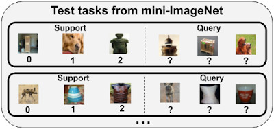
A popular dataset for studying few-shot classification is mini-ImageNet, a downsampled version of a subset of classes from ImageNet. This dataset contains 100 classes in total that are divided into training, validation and test class splits. While classes encountered at test time in benchmarks like mini-ImageNet have not been seen during training, they are still substantially similar to the training classes visually. Recent works reveal that this allows a model to perform competitively at test time simply by re-using features learned at training time, without necessarily demonstrating the capability to learn from the few examples presented to the model in the support set. In contrast, performing well on Meta-Dataset requires absorbing diverse information at training time and rapidly adapting it to solve significantly different tasks at test time that possibly originate from entirely unseen datasets.
Test tasks from mini-ImageNet. Each task is a classification problem between previously unseen (test) classes. The model can use the support set of a few labeled examples of the new classes to adapt to the task at hand and then predicts labels for the query examples of these new classes. The evaluation metric is the query set accuracy, averaged over examples within each task and across tasks.
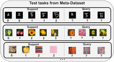
While other recent papers have investigated training on mini-ImageNet and evaluating on different datasets, Meta-Dataset represents the largest-scale organized benchmark for cross-dataset, few-shot image classification to date. It also introduces a sampling algorithm for generating tasks of varying characteristics and difficulty, by varying the number of classes in each task, the number of available examples per class, introducing class imbalances and, for some datasets, varying the degree of similarity between the classes of each task. Some example test tasks from Meta-Dataset are shown below.
Test tasks from Meta-Dataset. Contrary to the mini-ImageNet tasks shown above, different tasks here originate from (the test classes of) different datasets. Further, the number of classes and the support set sizes differ across tasks and the support sets might be class-imbalanced.
Initial Investigation and Findings on Meta-Dataset
We benchmark two main families of few-shot learning models on Meta-Dataset: pre-training and meta-learning.

Pre-training simply trains a classifier (a neural network feature extractor followed by a linear classifier) on the training set of classes using supervised learning. Then, the examples of a test task can be classified either by fine-tuning the pre-trained feature extractor and training a new task-specific linear classifier, or by means of nearest-neighbor comparisons, where the prediction for each query example is the label of its nearest support example. Despite its “baseline” status in the few-shot classification literature, this approach has recently enjoyed a surge of attention and competitive results.

On the other hand, meta-learners construct a number of “training tasks” and their training objective explicitly reflects the goal of performing well on each task’s query set after having adapted to that task using the associated support set, capturing the ability that is required at test time to solve each test task. Each training task is created by randomly sampling a subset of training classes and some examples of those classes to play the role of support and query sets.

Below, we summarize some of our findings from evaluating pre-training and meta-learning models on Meta Dataset:

1) Existing approaches have trouble leveraging heterogeneous training data sources.

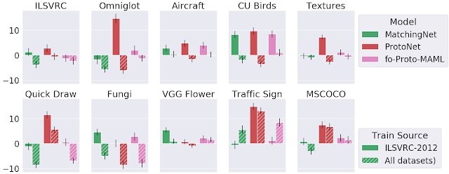
We compared training models (from both pre-training and meta-learning approaches) using only the training classes of ImageNet to using all training classes from the datasets in Meta-Dataset, in order to measure the generalization gain from using a more expansive collection of training data. We singled out ImageNet for this purpose, because the features learned on ImageNet readily transfer to other datasets. The evaluation tasks applied to all models are derived from a held-out set of classes from the datasets used in training, with at least two additional datasets that are entirely held-out for evaluation (i.e., no classes from these datasets were used for training).

One might expect that training on more data, albeit heterogeneous, would generalize better on the test set. However, this is not always the case. Specifically, the following figure displays the accuracy of different models on test tasks of Meta-Dataset’s ten datasets. We observe that the performance on test tasks coming from handwritten characters / doodles (Omniglot and Quickdraw) is significantly improved when having trained on all datasets, instead of ImageNet only. This is reasonable since these datasets are visually significantly different from ImageNet. However, for test tasks of natural image datasets, similar accuracy can be obtained by training on ImageNet only, revealing that current models cannot effectively leverage heterogeneous data towards improving in this regard.
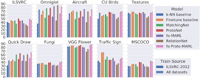
Comparison of test performance on each dataset after having trained on ImageNet (ILSVRC-2012) only or on all datasets.
2) Some models are more capable than others of exploiting additional data at test time.

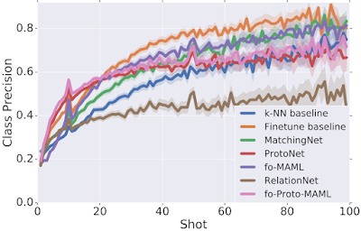
We analyzed the performance of different models as a function of the number of available examples in each test task, uncovering an interesting trade-off: different models perform best with a particular number of training (support) samples. We observe that some models outshine the rest when there are very few examples (“shots”) available (e.g., ProtoNet and our proposed fo-Proto-MAML) but don’t exhibit a large improvement when given more, while other models are not well-suited for tasks with very few examples but improve at a quicker rate as more are given (e.g., Finetune baseline). However, since in practice we might not know in advance the number of examples that will be available at test time, one would like to identify a model that can best leverage any number of examples, without disproportionately suffering in a particular regime.
Comparison of test performance averaged across different datasets to the number of examples available per class in test tasks (“shots”). Performance is measured in terms of class precision: the proportion of the examples of a class that are correctly labeled, averaged across classes.
3) The adaptation algorithm of a meta-learner is more heavily responsible for its performance than the fact that it is trained end-to-end (i.e. meta-trained).

We developed a new set of baselines to measure the benefit of meta-learning. Specifically, for several meta-learners, we consider a non-meta-learned counterpart that pre-trains a feature extractor and then, at evaluation time only, applies the same adaptation algorithm as the respective meta-learner on those features. When training on ImageNet only, meta-training often helps a bit or at least doesn’t hurt too much, but when training on all datasets, the results are mixed. This suggests that further work is needed to understand and improve upon meta-learning, especially across datasets.
Comparison of three different meta-learner variants to their corresponding inference-only baselines, when training on ImageNet (ILSVRC-1012) only or all datasets. Each bar represents the difference between meta-training and inference-only, so positive values indicate improved performance from meta-training.
Conclusion
Meta-Dataset introduces new challenges for few-shot classification. Our initial exploration has revealed limitations of existing methods, calling for additional research. Recent works have already reported exciting results on Meta-Dataset, for example using cleverly-designed task conditioning, more sophisticated hyperparameter tuning, a ‘meta-baseline’ that combines the benefits of pre-training and meta-learning, and finally using feature selection to specialize a universal representation for each task. We hope that Meta-Dataset will help drive research in this important sub-field of machine learning.

Acknowledgements
Meta-Dataset was developed by Eleni Triantafillou, Tyler Zhu, Vincent Dumoulin, Pascal Lamblin, Utku Evci, Kelvin Xu, Ross Goroshin, Carles Gelada, Kevin Swersky, Pierre-Antoine Manzagol and Hugo Larochelle. We would like to thank Pablo Castro for his valuable guidance on this blog post, Chelsea Finn for fruitful discussions and ensuring the correctness of fo-MAML’s implementation, as well as Zack Nado and Dan Moldovan for the initial dataset code that was adapted, Cristina Vasconcelos for spotting an issue in the ranking of models and John Bronskill for suggesting that we experiment with a larger inner-loop learning rate for MAML which indeed significantly improved our fo-MAML results.
Source: Google AI Blog


Contributing Data to Deepfake Detection Research


Deep learning has given rise to technologies that would have been thought impossible only a handful of years ago. Modern generative models are one example of these, capable of synthesizing hyperrealistic images, speech, music, and even video. These models have found use in a wide variety of applications, including making the world more accessible through text-to-speech, and helping generate training data for medical imaging.

Like any transformative technology, this has created new challenges. So-called "deepfakes"—produced by deep generative models that can manipulate video and audio clips—are one of these. Since their first appearance in late 2017, many open-source deepfake generation methods have emerged, leading to a growing number of synthesized media clips. While many are likely intended to be humorous, others could be harmful to individuals and society.

Google considers these issues seriously. As we published in our AI Principles last year, we are committed to developing AI best practices to mitigate the potential for harm and abuse. Last January, we announced our release of a dataset of synthetic speech in support of an international challenge to develop high-performance fake audio detectors. The dataset was downloaded by more than 150 research and industry organizations as part of the challenge, and is now freely available to the public.

Today, in collaboration with Jigsaw, we're announcing the release of a large dataset of visual deepfakes we've produced that has been incorporated into the Technical University of Munich and the University Federico II of Naples’ new FaceForensics benchmark, an effort that Google co-sponsors. The incorporation of these data into the FaceForensics video benchmark is in partnership with leading researchers, including Prof. Matthias Niessner, Prof. Luisa Verdoliva and the FaceForensics team. You can download the data on the FaceForensics github page.
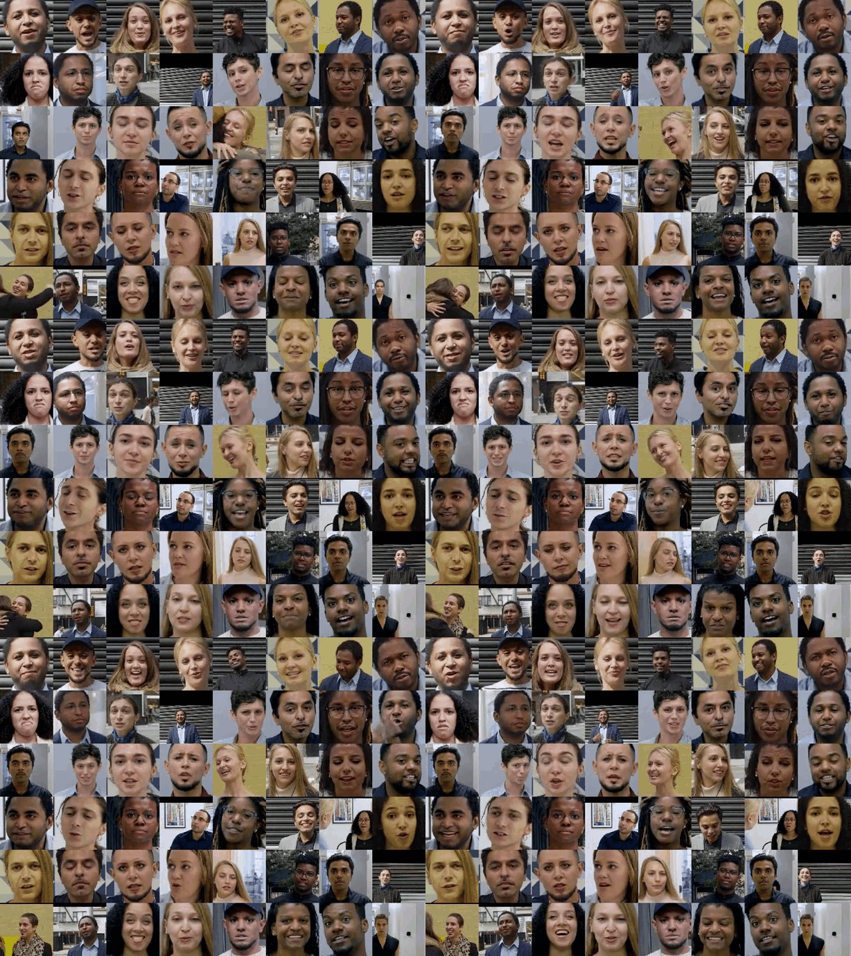
A sample of videos from Google’s contribution to the FaceForensics benchmark. To generate these, pairs of actors were selected randomly and deep neural networks swapped the face of one actor onto the head of another.
To make this dataset, over the past year we worked with paid and consenting actors to record hundreds of videos. Using publicly available deepfake generation methods, we then created thousands of deepfakes from these videos. The resulting videos, real and fake, comprise our contribution, which we created to directly support deepfake detection efforts. As part of the FaceForensics benchmark, this dataset is now available, free to the research community, for use in developing synthetic video detection methods.
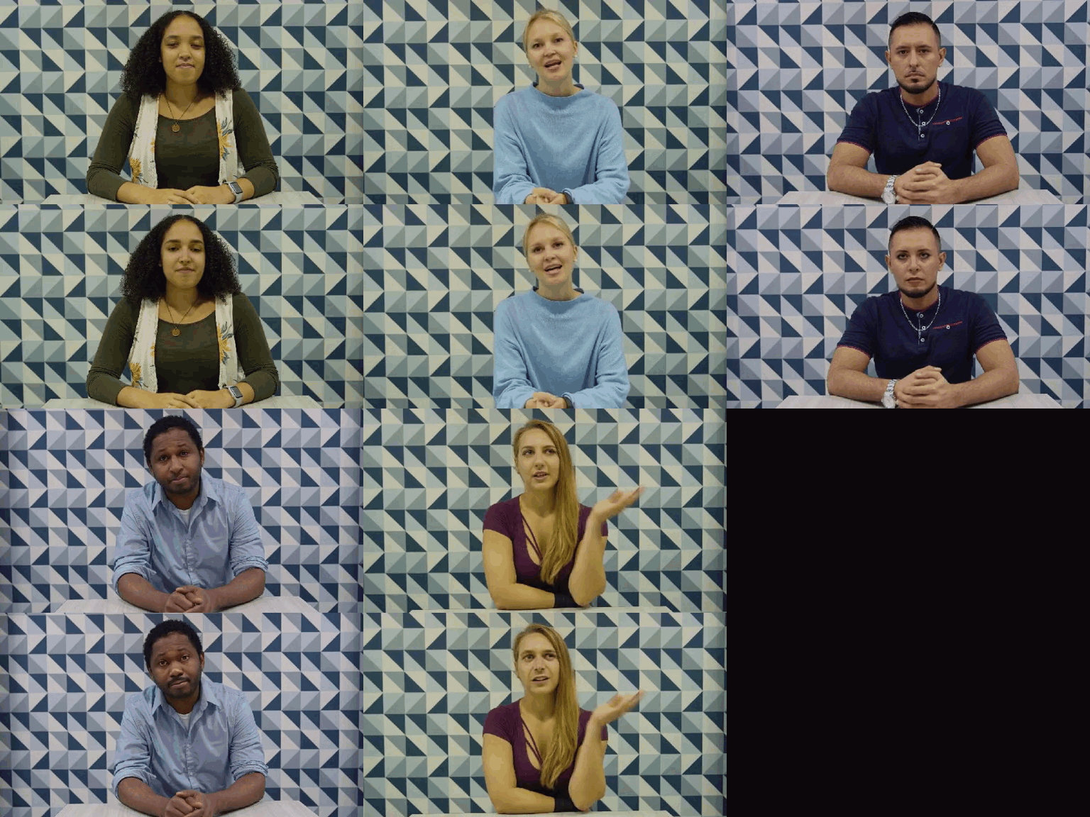
Actors were filmed in a variety of scenes. Some of these actors are pictured here (top) with an example deepfake (bottom), which can be a subtle or drastic change, depending on the other actor used to create them.
Since the field is moving quickly, we'll add to this dataset as deepfake technology evolves over time, and we’ll continue to work with partners in this space. We firmly believe in supporting a thriving research community around mitigating potential harms from misuses of synthetic media, and today's release of our deepfake dataset in the FaceForensics benchmark is an important step in that direction.

Acknowledgements
Special thanks to all our team members and collaborators who work on this project with us: Daisy Stanton, Per Karlsson, Alexey Victor Vorobyov, Thomas Leung, Jeremiah "Spudde" Childs, Christoph Bregler, Andreas Roessler, Davide Cozzolino, Justus Thies, Luisa Verdoliva, Matthias Niessner, and the hard-working actors and film crew who helped make this dataset possible.

Source: Google AI Blog


EfficientNet-EdgeTPU: Creating Accelerator-Optimized Neural Networks with AutoML


For several decades, computer processors have doubled their performance every couple of years by reducing the size of the transistors inside each chip, as described by Moore’s Law. As reducing transistor size becomes more and more difficult, there is a renewed focus in the industry on developing domain-specific architectures — such as hardware accelerators — to continue advancing computational power. This is especially true for machine learning, where efforts are aimed at building specialized architectures for neural network (NN) acceleration. Ironically, while there has been a steady proliferation of these architectures in data centers and on edge computing platforms, the NNs that run on them are rarely customized to take advantage of the underlying hardware.

Today, we are happy to announce the release of EfficientNet-EdgeTPU, a family of image classification models derived from EfficientNets, but customized to run optimally on Google’s Edge TPU, a power-efficient hardware accelerator available to developers through the Coral Dev Board and a USB Accelerator. Through such model customizations, the Edge TPU is able to provide real-time image classification performance while simultaneously achieving accuracies typically seen only when running much larger, compute-heavy models in data centers.

Using AutoML to customize EfficientNets for Edge TPU
EfficientNets have been shown to achieve state-of-the-art accuracy in image classification tasks while significantly reducing the model size and computational complexity. To build EfficientNets designed to leverage the Edge TPU’s accelerator architecture, we invoked the AutoML MNAS framework and augmented the original EfficientNet’s neural network architecture search space with building blocks that execute efficiently on the Edge TPU (discussed below). We also built and integrated a “latency predictor” module that provides an estimate of the model latency when executing on the Edge TPU, by running the models on a cycle-accurate architectural simulator. The AutoML MNAS controller implements a reinforcement learning algorithm to search this space while attempting to maximize the reward, which is a joint function of the predicted latency and model accuracy. From past experience, we know that Edge TPU’s power efficiency and performance tend to be maximized when the model fits within its on-chip memory. Hence we also modified the reward function to generate a higher reward for models that satisfy this constraint.
Overall AutoML flow for designing customized EfficientNet-EdgeTPU models.
Search Space Design
When performing the architecture search described above, one must consider that EfficientNets rely primarily on depthwise-separable convolutions, a type of neural network block that factorizes a regular convolution to reduce the number of parameters as well as the amount of computations. However, for certain configurations, a regular convolution utilizes the Edge TPU architecture more efficiently and executes faster, despite the much larger amount of compute. While it is possible, albeit tedious, to manually craft a network that uses an optimal combination of the different building blocks, augmenting the AutoML search space with these accelerator-optimal blocks is a more scalable approach.
A regular 3x3 convolution (right) has more compute (multiply-and-accumulate (mac) operations) than an depthwise-separable convolution (left), but for certain input/output shapes, executes faster on Edge TPU due to ~3x more effective hardware utilization.
In addition, removing certain operations from the search space that require modifications to the Edge TPU compiler to fully support, such swish non-linearity and squeeze-and-excitation block, naturally leads to models that are readily ported to the Edge TPU hardware. These operations tend to improve model quality slightly, so by eliminating them from the search space, we have effectively instructed AutoML to discover alternate network architectures that may compensate for any potential loss in quality.

Model Performance
The neural architecture search (NAS) described above produced a baseline model, EfficientNet-EdgeTPU-S, which is subsequently scaled up using EfficientNet's compound scaling method to produce the -M and -L models. The compound scaling approach selects an optimal combination of input image resolution scaling, network width, and depth scaling to construct larger, more accurate models. The -M, and -L models achieve higher accuracy at the cost of increased latency as shown in the figure below.
EfficientNet-EdgeTPU-S/M/L models achieve better latency and accuracy than existing EfficientNets (B1), ResNet, and Inception by specializing the network architecture for Edge TPU hardware. In particular, our EfficientNet-EdgeTPU-S achieves higher accuracy, yet runs 10x faster than ResNet-50.
Interestingly, the NAS-generated model employs the regular convolution quite extensively in the initial part of the network where the depthwise-separable convolution tends to be less effective than the regular convolution when executed on the accelerator. This clearly highlights the fact that trade-offs usually made while optimizing models for general purpose CPUs (reducing the total number of operations, for example) are not necessarily optimal for hardware accelerators. Also, these models achieve high accuracy even without the use of esoteric operations. Comparing with the other image classification models such as Inception-resnet-v2 and Resnet50, EfficientNet-EdgeTPU models are not only more accurate, but also run faster on Edge TPUs.

This work represents a first experiment in building accelerator-optimized models using AutoML. The AutoML-based model customization can be extended to not only a wide range of hardware accelerators, but also to several different applications that rely on neural networks.

From Cloud TPU training to Edge TPU deployment
We have released the training code and pretrained models for EfficientNet-EdgeTPU on our github repository. We employ tensorflow’s post-training quantization tool to convert a floating-point trained model to an Edge TPU-compatible integer-quantized model. For these models, the post-training quantization works remarkably well and produces only a very slight loss in accuracy (~0.5%). The script for exporting the quantized model from a training checkpoint can be found here. For an update on the Coral platform, see this post on the Google Developer’s Blog, and for full reference materials and detailed instructions, please refer to the Coral website.

Acknowledgements
Special thanks to Quoc Le, Hongkun Yu, Yunlu Li, Ruoming Pang, and Vijay Vasudevan from the Google Brain team; Bo Wu, Vikram Tank, and Ajay Nair from the Google Coral team; Han Vanholder, Ravi Narayanaswami, John Joseph, Dong Hyuk Woo, Raksit Ashok, Jason Jong Kyu Park, Jack Liu, Mohammadali Ghodrat, Cao Gao, Berkin Akin, Liang-Yun Wang, Chirag Gandhi, and Dongdong Li from the Google Edge TPU team.

Source: Google AI Blog


An Inside Look at Google Earth Timelapse


Six years ago, we first introduced Google Earth Timelapse, a global, zoomable time-lapse video that lets anyone explore our changing planet’s surface—from the global scale to the local scale. Earth Timelapse consists of 83 million multi-resolution overlapping video tiles, which are made interactively explorable through the open-source Time Machine client software developed at Carnegie Mellon University’s CREATE Lab. At its core, Google Earth Timelapse is an example of how organizing information can make it more accessible and useful, turning petabytes of satellite imagery into an interactive experience that shows the dynamic changes occurring across space and time.
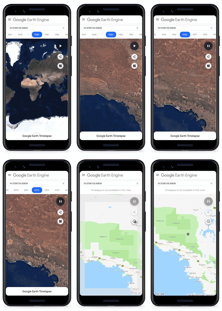
In April, we introduced several updates to Timelapse, including two additional years of imagery to the time-series visualization, which now spans from 1984 to 2018, with visual upgrades that make exploring more accessible and intuitive. We are especially excited that this update includes support for mobile and tablet devices, which are quickly overtaking desktop computers as the dominant source of app traffic.

Building the Global Visualization
Making a planetary-sized time-lapse video required a significant amount of pixel crunching in Earth Engine, Google's cloud platform for petabyte-scale geospatial analysis. The new release followed a process similar to what we did in 2013, but at a significantly greater scale—turning 15 million satellite images acquired over the last three and a half decades from the USGS/NASA Landsat and European Sentinel programs into 35 cloud-free 4-terapixel images of the planet—one for each year from 1984 to 2018.
At its native resolution, the Timelapse visualization is a 4 terapixel video (that's four trillion pixels), which would take about 12 days to download on a 95 Mb/s internet connection. Most computers would have difficulty playing a video of this size, let alone with an interactive, zoomable interface. The problem is even more severe for a mobile device.

A solution was pioneered by Google Maps in 2004 with the map pyramiding technique. Before that time, navigating a map required the use of directional arrows to pan and zoom, with each step requiring the page to reload. The map pyramiding technique assembles the full map image displayed on-screen from tens of small 256x256 pixel non-overlapping image tiles in an array, with new tiles fetched as needed at an appropriate resolution as the user pans and zooms across the map.
A traditional Mercator map pyramid contains non-overlapping image tiles.
This works very well for maps made of static images, but less so for pyramids of video tiles, such as those used by Timelapse, since it requires a web browser to keep up to 16 videos in sync while interacting with the visualization. The solution is embodied in CREATE Lab’s open source Time Machine software: create much larger video tiles that can cover the entire screen and only show one whole-screen tile at a time. The tiles create a pyramid, where sibling tiles overlap with their neighbors to provide a seamless transition between tiles while panning and zooming. Though the overlapping tiles require the use of about 16x more videos, this pyramid structure enables the use of Timelapse on mobile devices by minimizing the amount of data required for visualization.

In our newest release, the global video pyramid consists of 83 million videos across 13 zoom levels, which required about 2 million CPU hours distributed across thousands of machines in Google Cloud to generate.
Earth Timelapse uses a pyramid of overlapping video tiles.
Time Travel, Wherever You Are
Prior to April's update, ~30% of visitors to the Timelapse visualization were on mobile devices and didn't actually experience the visualization; instead they saw a YouTube playlist of locations in Timelapse. Until recently, the hardware and CPUs for phones and tablets could not decode videos fast enough without significant delays when someone attempted to zoom in or pan across a video, making mobile exploration unpleasant, if not impossible. In addition, in order for the visualization to be smooth as you pan and zoom, each video that is loaded must sync to the previously playing video and begin playing automatically. But, until only recently, mobile browser vendors had disabled video autoplay at the browser level for bandwidth reasons.

Now that mobile browser vendors have re-enabled video autoplay, we are able to take advantage of current mobile hardware and CPU capabilities, while leveraging the pyramid mapping technique’s efficient use of data, to enable Timelapse on mobile.

Redesigning Timelapse for Exploration Across Devices
Timelapse is a tool for exploration, so we designed for immersiveness, devoting as much real estate as possible to the map. On the other hand, it's not just a map, but a map of videos. So we kept controls visible, like pausing and restarting the timeline or choosing highlights, by leveraging Material Design with simple, clean lines and clear focal areas.
Navigate with Google Maps using the new "Maps Mode" toggle.
To explore, you need to know where you are or where somewhere else is, so the new interface includes a new "Maps Mode" toggle that lets the user navigate with Google Maps. We also built in scalability to the timeline element of the UI, so that new features added in the future, such as lengthening the time-lapse or adding options for different time increments, won’t break the design. The timeline also allows the user to go backwards in time—an interesting way to compare the present with the past.

For desktop browsers supporting WebGL, we also added a new WebGL viewer to the open source project, which loads and synchronizes multiple videos to fill the screen at optimal resolution. The aesthetic improvement of this is nontrivial, with >4x better resolution.

What's next
We're excited about the abundance of freely available, openly licensed satellite imagery and remote sensing data available, enabling new visualizations across time, space, and the visual and non-visual spectrum. We've found it's often the data combined with supplemental layers, such as the World Database on Protected Areas (WDPA) boundaries, that can spark new insights. For example, seeing the visual connection between declining home ownership and shifts in the city of Pittsburgh's racial makeup tells a story about inequality that numbers on a page simply cannot. Visual evidence can transcend language and cultural barriers and, we hope, generate productive conversations about our global challenges.

Acknowledgements
Randy Sargent, Senior Systems Scientist, Carnegie Mellon University CREATE Lab and the Google Earth Engine team

Source: Google AI Blog


Announcing Google-Landmarks-v2: An Improved Dataset for Landmark Recognition & Retrieval


Last year we released Google-Landmarks, the largest world-wide landmark recognition dataset available at that time. In order to foster advancements in research on instance-level recognition (recognizing specific instances of objects, e.g. distinguishing Niagara Falls from just any waterfall) and image retrieval (matching a specific object in an input image to all other instances of that object in a catalog of reference images), we also hosted two Kaggle challenges, Landmark Recognition 2018 and Landmark Retrieval 2018, in which more than 500 teams of researchers and machine learning (ML) enthusiasts participated. However, both instance recognition and image retrieval methods require ever larger datasets in both the number of images and the variety of landmarks in order to train better and more robust systems.

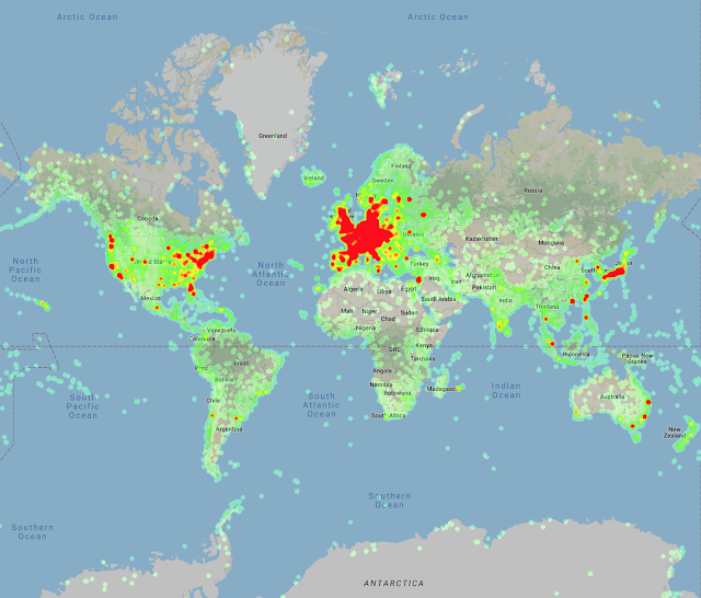
In support of this goal, this year we are releasing Google-Landmarks-v2, a completely new, even larger landmark recognition dataset that includes over 5 million images (2x that of the first release) of more than 200 thousand different landmarks (an increase of 7x). Due to the difference in scale, this dataset is much more diverse and creates even greater challenges for state-of-the-art instance recognition approaches. Based on this new dataset, we are also announcing two new Kaggle challenges—Landmark Recognition 2019 and Landmark Retrieval 2019—and releasing the source code and model for Detect-to-Retrieve, a novel image representation suitable for retrieval of specific object instances.
Heatmap of the landmark locations in Google-Landmarks-v2, which demonstrates the increase in the scale of the dataset and the improved geographic coverage compared to last year’s dataset.
Creating the Dataset
A particular problem in preparing Google-Landmarks-v2 was the generation of instance labels for the landmarks represented, since it is virtually impossible for annotators to recognize all of the hundreds of thousands of landmarks that could potentially be present in a given photo. Our solution to this problem was to crowdsource the landmark labeling through the efforts of a world-spanning community of hobby photographers, each familiar with the landmarks in their region.
Selection of images from Google-Landmarks-v2. Landmarks include (left to right, top to bottom) Neuschwanstein Castle, Golden Gate Bridge, Kiyomizu-dera, Burj khalifa, Great Sphinx of Giza, and Machu Picchu.
Another issue for research datasets is the requirement that images be shared freely and stored indefinitely, so that the dataset can be used to track the progress of research over a long period of time. As such, we sourced the Google-Landmarks-v2 images through Wikimedia Commons, capturing both world-famous and lesser-known, local landmarks while ensuring broad geographic coverage (thanks in part to Wiki Loves Monuments) and photos sourced from public institutions, including historical photographs that are valuable to test instance recognition over time.

The Kaggle Challenges
The goal of the Landmark Recognition 2019 challenge is to recognize a landmark presented in a query image, while the goal of Landmark Retrieval 2019 is to find all images showing that landmark. The challenges include cash prizes totaling $50,000 and the winning teams will be invited to present their methods at the Second Landmark Recognition Workshop at CVPR 2019.

Open Sourcing our Model
To foster research reproducibility and help push the field of instance recognition forward, we are also releasing open-source code for our new technique, called Detect-to-Retrieve (which will be presented as a paper in CVPR 2019). This new method leverages bounding boxes from an object detection model to give extra weight to image regions containing the class of interest, which significantly improves accuracy. The model we are releasing is trained on a subset of 86k images from the original Google-Landmarks dataset that were annotated with landmark bounding boxes. We are making these annotations available along with the original dataset here.

We invite researchers and ML enthusiasts to participate in the Landmark Recognition 2019 and Landmark Retrieval 2019 Kaggle challenges and to join the Second Landmark Recognition Workshop at CVPR 2019. We hope that this dataset will help advance the state-of-the-art in instance recognition and image retrieval. The data is being made available via the Common Visual Data Foundation.

Acknowledgments
The core contributors to this project are Andre Araujo, Bingyi Cao, Jack Sim and Tobias Weyand. We would like to thank our team members Daniel Kim, Emily Manoogian, Nicole Maffeo, and Hartwig Adam for their kind help. Thanks also to Marvin Teichmann and Menglong Zhu for their contribution to collecting the landmark bounding boxes and developing the Detect-to-Retrieve technique. We would like to thank Will Cukierski and Maggie Demkin for their help organizing the Kaggle challenge, Elan Hourticolon-Retzler, Yuan Gao, Qin Guo, Gang Huang, Yan Wang, Zhicheng Zheng for their help with data collection, Tsung-Yi Lin for his support with CVDF hosting, as well as our CVPR workshop co-organizers Bohyung Han, Shih-Fu Chang, Ondrej Chum, Torsten Sattler, Giorgos Tolias, and Xu Zhang. We have great appreciation for the Wikimedia Commons Community and their volunteer contributions to an invaluable photographic archive of the world’s cultural heritage. And finally, we’d like to thank the Common Visual Data Foundation for hosting the dataset.

Source: Google AI Blog


Exploring Neural Networks with Activation Atlases


Neural networks have become the de facto standard for image-related tasks in computing, currently being deployed in a multitude of scenarios, ranging from automatically tagging photos in your image library to autonomous driving systems. These machine-learned systems have become ubiquitous because they perform more accurately than any system humans were able to directly design without machine learning. But because essential details of these systems are learned during the automated training process, understanding how a network goes about its given task can sometimes remain a bit of a mystery.

Today, in collaboration with colleagues at OpenAI, we're publishing "Exploring Neural Networks with Activation Atlases", which describes a new technique aimed at helping to answer the question of what image classification neural networks "see" when provided an image. Activation atlases provide a new way to peer into convolutional vision networks, giving a global, hierarchical, and human-interpretable overview of concepts within the hidden layers of a network. We think of activation atlases as revealing a machine-learned alphabet for images — an array of simple, atomic concepts that are combined and recombined to form much more complex visual ideas. We are also releasing some jupyter notebooks to help you get you started in making your own activation atlases.

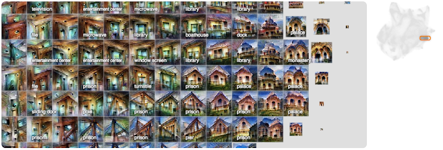
A detail view of an activation atlas from one of the layers of the InceptionV1 vision classification network. It reveals many of the visual detectors that the network uses to classify images, such as different types of fruit-like textures, honeycomb patterns and fabric-like textures.
The activation atlases shown below are built from a convolutional image classification network, Inceptionv1, that was trained on the ImageNet dataset. In general, classification networks are shown an image and then asked to give that image a label from one of 1,000 predetermined classes — such as "carbonara", "snorkel" or "frying pan". To do this, our network evaluates the image data progressively through about ten layers, each made of hundreds of neurons that each activate to varying degrees on different types of image patches. One neuron at one layer might respond positively to a dog's ear, another at an earlier layer might respond to a high-contrast vertical line.

An activation atlas is built by collecting the internal activations from each of these layers of our neural network from one million images. These activations, represented by a complex set of high-dimensional vectors, is projected into useful 2D layouts via UMAP, a dimensionality-reduction technique that preserving some of the local structure of the original high-dimensional space.

This takes care of organizing our activation vectors, but we also need to aggregate them into a more manageable number — all the activations are too many to consume at a glance. To do this, we draw a grid over the 2D layout we created. For each cell in our grid, we average all the activations that lie within the boundaries of that cell, and use feature visualization to create an iconic representation.
Left: A randomized set of one million images is fed through the network, collecting one random spatial activation per image. Center: The activations are fed through UMAP to reduce them to two dimensions. They are then plotted, with similar activations placed near each other. Right: We then draw a grid, average the activations that fall within a cell, and run feature inversion on the averaged activation.
Below we can see an activation atlas for just one layer in a neural network (remember that these classification models can have half a dozen or more layers). It reveals a universe of the visual concepts the network has learned to classify images at this layer. This atlas can be a bit overwhelming at first glance — there's a lot going on! This diversity is a reflection of the variety of visual abstractions and concepts the model has developed.
An overview of an activation atlas for one of the many layers (mixed4c) within Inception v1. It is about halfway through the network.
In this detail, we can see detectors for different types of leaves and plants.
Here we can see different detectors for water, lakes and sandbars.
Here we see different types of buildings and bridges.
As we mentioned before, there are many more layers in this network. Let's look at the layers that came before this one to see how these concepts become more refined as we go deeper into the network (Each layer builds its activations on top of the preceding layer's activations).
In an early layer, mixed4a, there is a vague "mammalian" area.
By the next layer in the network, mixed4b, animals and people have been disentangled, with some fruit and food emerging in the middle.
By layer mixed4c these concepts are further refined and differentiated into small "peninsulas".
Here we've seen the global structure evolve from layer to layer, but each of the individual concepts also become more specific and complex from layer to layer. If we focus on the areas of three layers that contribute to a specific classification, say "cabbage", we can see this clearly.
Left: This early layer is very nonspecific in comparison to the others. Center: By the middle layer, the images definitely resemble leaves, but they could be any type of plant. Right: By the last layer the images are very specific to cabbage, leaves curved into rounded balls.
There is another phenomenon worth noting: not only are concepts being refined as you move from layer to layer, but new concepts seem to be appearing out of combinations of old ones.
You can see how sand and water are distinct concepts in a middle layer, mixed4c (left and center), both with strong attributions to the classification of "sandbar". Contrast this with a later layer (right), mixed5b, where the two ideas seem to be fused into one activation.
Instead of zooming in on certain areas of the whole atlas for a specific layer, we can also create an atlas at a specific layer for just one of the 1,000 classes in ImageNet. This will show the concepts and detectors that the network most often uses to classify a specific class, say "red fox" for instance.
Here we can more clearly see what the network is focusing on to classify a "red fox". There are pointy ears, white snouts surrounded by red fur, and wooded or snowy backgrounds.
Here we can see the many different scales and angles of detectors for "tile roof".
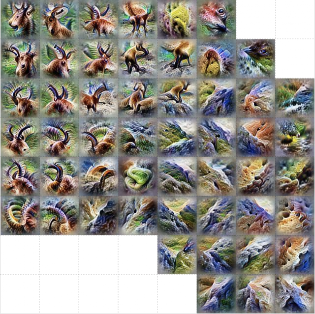
For "ibex", we see detectors for horns and brown fur, but also environments where we might find such animals, like rocky hillsides.
Like the detectors for tile roof, "artichoke" also has many different sizes of detectors for the texture of an artichoke, but we also get some purple flower detectors. These are presumably detecting the blossoms of an artichoke plant.
These atlases not only reveal nuanced visual abstractions within a model, but they can also reveal high-level misunderstandings. For example, by looking at an activation atlas for a "great white shark" we water and triangular fins (as expected) but we also see something that looks like a baseball. This hints at a shortcut taken by this research model where it conflates the red baseball stitching with the open mouth of a great white shark.
We can test this by using a patch of an image of a baseball to switch the model's classification of a particular image from "grey whale" to "great white shark".
We hope that activation atlases will be a useful tool in the quiver of techniques that are making machine learning more accessible and interpretable. To help you get started, we've released several jupyter notebooks which can be executed immediately in your browser with one click via colab. They build upon the previously released toolkit Lucid, which includes code for many other interpretability visualization techniques included as well. We're excited to see what you discover!

Source: Google AI Blog


Introducing the Inclusive Images Competition


The release of large, publicly available image datasets, such as ImageNet, Open Images and Conceptual Captions, has been one of the factors driving the tremendous progress in the field of computer vision. While these datasets are a necessary and critical part of developing useful machine learning (ML) models, some open source data sets have been found to be geographically skewed based on how they were collected. Because the shape of a dataset informs what an ML model learns, such skew may cause the research community to inadvertently develop models that may perform less well on images drawn from geographical regions under-represented in those data sets. For example, the images below show one standard open-source image classifier trained on the Open Images dataset that does not properly apply “wedding” related labels to images of wedding traditions from different parts of the world.
Wedding photographs (donated by Googlers), labeled by a classifier trained on the Open Images dataset. The classifier’s label predictions are recorded below each image.
While Google is focusing on building even more representative datasets, we also want to encourage additional research in the field around ways that machine learning methods can be more robust and inclusive when learning from imperfect data sources. This is an important research challenge, and one that pushes the boundaries of ways that machine learning models are currently created. Good solutions will help ensure that even when some data sources aren’t fully inclusive, the models developed with them can be.

In support of this effort and to spur further progress in developing inclusive ML models, we are happy to announce the Inclusive Images Competition on Kaggle. Developed in partnership with the Conference on Neural Information Processing Systems Competition Track, this competition challenges you to use Open Images, a large, multilabel, publicly-available image classification dataset that is majority-sampled from North America and Europe, to train a model that will be evaluated on images collected from a different set of geographic regions across the globe.
The three geographical distributions of data in this competition. Competitors will train their models on Open Images, a widely used publicly available benchmark dataset for image classification which happens to be drawn mostly from North America and Western Europe. Models are then evaluated first on Challenge Stage 1 and finally on Challenge Stage 2, each with different un-revealed geographical distributions. In this way, models are stress-tested for their ability to operate inclusively beyond their training data.
For model evaluation, we have created two Challenge datasets via our Crowdsource project, where we asked our volunteers from across the globe to participate in contributing photos of their surroundings. We hope that these datasets, built by donations from Google’s global community, will provide a challenging geographically-based stress test for this competition. We also plan to release a larger set of images at the end of the competition to further encourage inclusive development, with more inclusive data.
Examples of labeled images from the challenge dataset. Clockwise from top left, image donation by Peter Tester, Mukesh Kumhar, HeeYoung Moon, Sudipta Pramanik, jaturan amnatbuddee, Tomi Familoni and Anu Subhi
The Inclusive Images Competition officially started September 5th with the available training data & first stage Challenge data set. The deadline for submitting your results will be Monday, November 5th, and the test set will be released on Tuesday, November 6th. For more details and timelines, please visit the Inclusive Images Competition website.

The results of the competition will be presented at the 2018 Conference on Neural Information Processing Systems, and we will provide top-ranking competitors with travel grants to attend the conference (see this page for full details). We look forward to being part of the community's development of more inclusive, global image classification algorithms!

Acknowledgements
We would like to thank the following individuals for making the Inclusive Image Competition and dataset possible: James Atwood, Pallavi Baljekar, Parker Barnes, Anurag Batra, Eric Breck, Peggy Chi, Tulsee Doshi, Julia Elliott, Gursheesh Kaur, Akshay Gaur, Yoni Halpern, Henry Jicha, Matthew Long, Jigyasa Saxena, and D. Sculley.

Source: Google AI Blog


Using Evolutionary AutoML to Discover Neural Network Architectures


The brain has evolved over a long time, from very simple worm brains 500 million years ago to a diversity of modern structures today. The human brain, for example, can accomplish a wide variety of activities, many of them effortlessly — telling whether a visual scene contains animals or buildings feels trivial to us, for example. To perform activities like these, artificial neural networks require careful design by experts over years of difficult research, and typically address one specific task, such as to find what's in a photograph, to call a genetic variant, or to help diagnose a disease. Ideally, one would want to have an automated method to generate the right architecture for any given task.

One approach to generate these architectures is through the use of evolutionary algorithms. Traditional research into neuro-evolution of topologies (e.g. Stanley and Miikkulainen 2002) has laid the foundations that allow us to apply these algorithms at scale today, and many groups are working on the subject, including OpenAI, Uber Labs, Sentient Labs and DeepMind. Of course, the Google Brain team has been thinking about AutoML too. In addition to learning-based approaches (eg. reinforcement learning), we wondered if we could use our computational resources to programmatically evolve image classifiers at unprecedented scale. Can we achieve solutions with minimal expert participation? How good can today's artificially-evolved neural networks be? We address these questions through two papers.

In “Large-Scale Evolution of Image Classifiers,” presented at ICML 2017, we set up an evolutionary process with simple building blocks and trivial initial conditions. The idea was to "sit back" and let evolution at scale do the work of constructing the architecture. Starting from very simple networks, the process found classifiers comparable to hand-designed models at the time. This was encouraging because many applications may require little user participation. For example, some users may need a better model but may not have the time to become machine learning experts. A natural question to consider next was whether a combination of hand-design and evolution could do better than either approach alone. Thus, in our more recent paper, “Regularized Evolution for Image Classifier Architecture Search” (2018), we participated in the process by providing sophisticated building blocks and good initial conditions (discussed below). Moreover, we scaled up computation using Google's new TPUv2 chips. This combination of modern hardware, expert knowledge, and evolution worked together to produce state-of-the-art models on CIFAR-10 and ImageNet, two popular benchmarks for image classification.

A Simple Approach
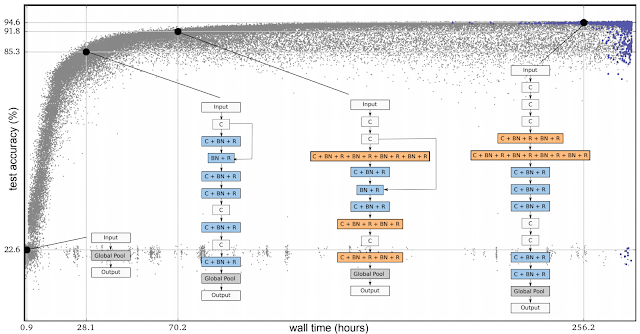
The following is an example of an experiment from our first paper. In the figure below, each dot is a neural network trained on the CIFAR-10 dataset, which is commonly used to train image classifiers. Initially, the population consists of one thousand identical simple seed models (no hidden layers). Starting from simple seed models is important — if we had started from a high-quality model with initial conditions containing expert knowledge, it would have been easier to get a high-quality model in the end. Once seeded with the simple models, the process advances in steps. At each step, a pair of neural networks is chosen at random. The network with higher accuracy is selected as a parent and is copied and mutated to generate a child that is then added to the population, while the other neural network dies out. All other networks remain unchanged during the step. With the application of many such steps in succession, the population evolves.
Progress of an evolution experiment. Each dot represents an individual in the population. The four diagrams show examples of discovered architectures. These correspond to the best individual (rightmost; selected by validation accuracy) and three of its ancestors.
The mutations in our first paper are purposefully simple: remove a convolution at random, add a skip connection between arbitrary layers, or change the learning rate, to name a few. This way, the results show the potential of the evolutionary algorithm, as opposed to the quality of the search space. For example, if we had used a single mutation that transforms one of the seed networks into an Inception-ResNet classifier in one step, we would be incorrectly concluding that the algorithm found a good answer. Yet, in that case, all we would have done is hard-coded the final answer into a complex mutation, rigging the outcome. If instead we stick with simple mutations, this cannot happen and evolution is truly doing the job. In the experiment in the figure, simple mutations and the selection process cause the networks to improve over time and reach high test accuracies, even though the test set had never been seen during the process. In this paper, the networks can also inherit their parent's weights. Thus, in addition to evolving the architecture, the population trains its networks while exploring the search space of initial conditions and learning-rate schedules. As a result, the process yields fully trained models with optimized hyperparameters. No expert input is needed after the experiment starts.

In all the above, even though we were minimizing the researcher's participation by having simple initial architectures and intuitive mutations, a good amount of expert knowledge went into the building blocks those architectures were made of. These included important inventions such as convolutions, ReLUs and batch-normalization layers. We were evolving an architecture made up of these components. The term "architecture" is not accidental: this is analogous to constructing a house with high-quality bricks.

Combining Evolution and Hand Design
After our first paper, we wanted to reduce the search space to something more manageable by giving the algorithm fewer choices to explore. Using our architectural analogy, we removed all the possible ways of making large-scale errors, such as putting the wall above the roof, from the search space. Similarly with neural network architecture searches, by fixing the large-scale structure of the network, we can help the algorithm out. So how to do this? The inception-like modules introduced in Zoph et al. (2017) for the purpose of architecture search proved very powerful. Their idea is to have a deep stack of repeated modules called cells. The stack is fixed but the architecture of the individual modules can change.
The building blocks introduced in Zoph et al. (2017). The diagram on the left is the outer structure of the full neural network, which parses the input data from bottom to top through a stack of repeated cells. The diagram on the right is the inside structure of a cell. The goal is to find a cell that yields an accurate network.
In our second paper, “Regularized Evolution for Image Classifier Architecture Search” (2018), we presented the results of applying evolutionary algorithms to the search space described above. The mutations modify the cell by randomly reconnecting the inputs (the arrows on the right diagram in the figure) or randomly replacing the operations (for example, they can replace the "max 3x3" in the figure, a max-pool operation, with an arbitrary alternative). These mutations are still relatively simple, but the initial conditions are not: the population is now initialized with models that must conform to the outer stack of cells, which was designed by an expert. Even though the cells in these seed models are random, we are no longer starting from simple models, which makes it easier to get to high-quality models in the end. If the evolutionary algorithm is contributing meaningfully, the final networks should be significantly better than the networks we already know can be constructed within this search space. Our paper shows that evolution can indeed find state-of-the-art models that either match or outperform hand-designs.

A Controlled Comparison
Even though the mutation/selection evolutionary process is not complicated, maybe an even more straightforward approach (like random search) could have done the same. Other alternatives, though not simpler, also exist in the literature (like reinforcement learning). Because of this, the main purpose of our second paper was to provide a controlled comparison between techniques.
Comparison between evolution, reinforcement learning, and random search for the purposes of architecture search. These experiments were done on the CIFAR-10 dataset, under the same conditions as Zoph et al. (2017), where the search space was originally used with reinforcement learning.
The figure above compares evolution, reinforcement learning, and random search. On the left, each curve represents the progress of an experiment, showing that evolution is faster than reinforcement learning in the earlier stages of the search. This is significant because with less compute power available, the experiments may have to stop early. Moreover evolution is quite robust to changes in the dataset or search space. Overall, the goal of this controlled comparison is to provide the research community with the results of a computationally expensive experiment. In doing so, it is our hope to facilitate architecture searches for everyone by providing a case study of the relationship between the different search algorithms. Note, for example, that the figure above shows that the final models obtained with evolution can reach very high accuracy while using fewer floating-point operations.

One important feature of the evolutionary algorithm we used in our second paper is a form of regularization: instead of letting the worst neural networks die, we remove the oldest ones — regardless of how good they are. This improves robustness to changes in the task being optimized and tends to produce more accurate networks in the end. One reason for this may be that since we didn't allow weight inheritance, all networks must train from scratch. Therefore, this form of regularization selects for networks that remain good when they are re-trained. In other words, because a model can be more accurate just by chance — noise in the training process means even identical architectures may get different accuracy values — only architectures that remain accurate through the generations will survive in the long run, leading to the selection of networks that retrain well. More details of this conjecture can be found in the paper.

The state-of-the-art models we evolved are nicknamed AmoebaNets, and are one of the latest results from our AutoML efforts. All these experiments took a lot of computation — we used hundreds of GPUs/TPUs for days. Much like a single modern computer can outperform thousands of decades-old machines, we hope that in the future these experiments will become household. Here we aimed to provide a glimpse into that future.

Acknowledgements
We would like to thank Alok Aggarwal, Yanping Huang, Andrew Selle, Sherry Moore, Saurabh Saxena, Yutaka Leon Suematsu, Jie Tan, Alex Kurakin, Quoc Le, Barret Zoph, Jon Shlens, Vijay Vasudevan, Vincent Vanhoucke, Megan Kacholia, Jeff Dean, and the rest of the Google Brain team for the collaborations that made this work possible.

Source: Google AI Blog