Tag Archives: Google Brain

Applying Deep Learning to Metastatic Breast Cancer Detection


A pathologist’s microscopic examination of a tumor in patients is considered the gold standard for cancer diagnosis, and has a profound impact on prognosis and treatment decisions. One important but laborious aspect of the pathologic review involves detecting cancer that has spread (metastasized) from the primary site to nearby lymph nodes. Detection of nodal metastasis is relevant for most cancers, and forms one of the foundations of the widely-used TNM cancer staging.

In breast cancer in particular, nodal metastasis influences treatment decisions regarding radiation therapy, chemotherapy, and the potential surgical removal of additional lymph nodes. As such, the accuracy and timeliness of identifying nodal metastases has a significant impact on clinical care. However, studies have shown that about 1 in 4 metastatic lymph node staging classifications would be changed upon second pathologic review, and detection sensitivity of small metastases on individual slides can be as low as 38% when reviewed under time constraints.

Last year, we described our deep learning–based approach to improve diagnostic accuracy (LYmph Node Assistant, or LYNA) to the 2016 ISBI Camelyon Challenge, which provided gigapixel-sized pathology slides of lymph nodes from breast cancer patients for researchers to develop computer algorithms to detect metastatic cancer. While LYNA achieved significantly higher cancer detection rates (Liu et al. 2017) than had been previously reported, an accurate algorithm alone is insufficient to improve pathologists’ workflow or improve outcomes for breast cancer patients. For patient safety, these algorithms must be tested in a variety of settings to understand their strengths and weaknesses. Furthermore, the actual benefits to pathologists using these algorithms had not been previously explored and must be assessed to determine whether or not an algorithm actually improves efficiency or diagnostic accuracy.

In “Artificial Intelligence Based Breast Cancer Nodal Metastasis Detection: Insights into the Black Box for Pathologists” (Liu et al. 2018), published in the Archives of Pathology and Laboratory Medicine and “Impact of Deep Learning Assistance on the Histopathologic Review of Lymph Nodes for Metastatic Breast Cancer” (Steiner, MacDonald, Liu et al. 2018) published in The American Journal of Surgical Pathology, we present a proof-of-concept pathologist assistance tool based on LYNA, and investigate these factors.

In the first paper, we applied our algorithm to de-identified pathology slides from both the Camelyon Challenge and an independent dataset provided by our co-authors at the Naval Medical Center San Diego. Because this additional dataset consisted of pathology samples from a different lab using different processes, it improved the representation of the diversity of slides and artifacts seen in routine clinical practice. LYNA proved robust to image variability and numerous histological artifacts, and achieved similar performance on both datasets without additional development.
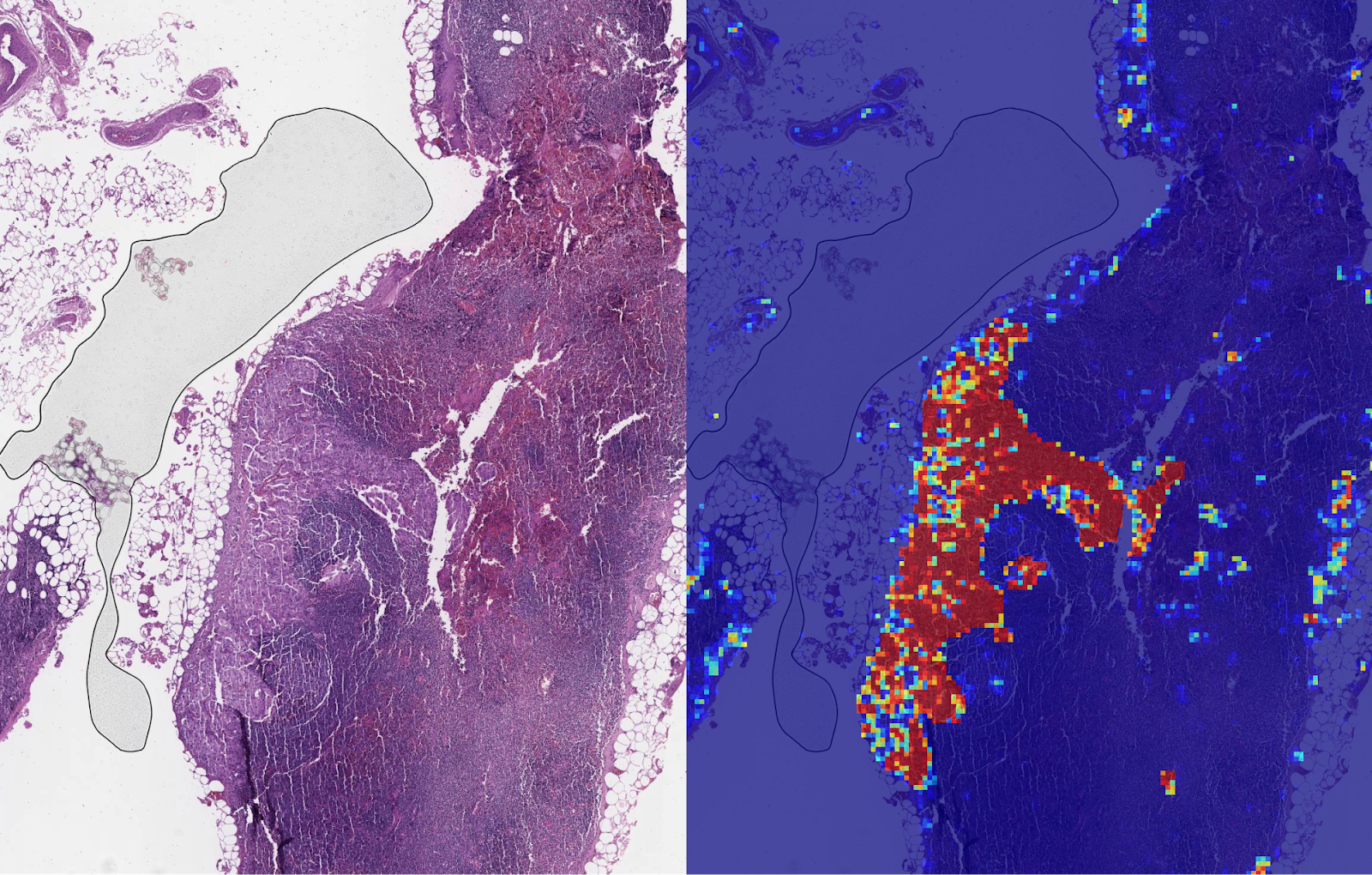
Left: sample view of a slide containing lymph nodes, with multiple artifacts: the dark zone on the left is an air bubble, the white streaks are cutting artifacts, the red hue across some regions are hemorrhagic (containing blood), the tissue is necrotic (decaying), and the processing quality was poor. Right: LYNA identifies the tumor region in the center (red), and correctly classifies the surrounding artifact-laden regions as non-tumor (blue).
In both datasets, LYNA was able to correctly distinguish a slide with metastatic cancer from a slide without cancer 99% of the time. Further, LYNA was able to accurately pinpoint the location of both cancers and other suspicious regions within each slide, some of which were too small to be consistently detected by pathologists. As such, we reasoned that one potential benefit of LYNA could be to highlight these areas of concern for pathologists to review and determine the final diagnosis.

In our second paper, 6 board-certified pathologists completed a simulated diagnostic task in which they reviewed lymph nodes for metastatic breast cancer both with and without the assistance of LYNA. For the often laborious task of detecting small metastases (termed micrometastases), the use of LYNA made the task subjectively “easier” (according to pathologists’ self-reported diagnostic difficulty) and halved average slide review time, requiring about one minute instead of two minutes per slide.
Left: sample views of a slide containing lymph nodes with a small metastatic breast tumor at progressively higher magnifications. Right: the same views when shown with algorithmic “assistance” (LYmph Node Assistant, LYNA) outlining the tumor in cyan.
This suggests the intriguing potential for assistive technologies such as LYNA to reduce the burden of repetitive identification tasks and to allow more time and energy for pathologists to focus on other, more challenging clinical and diagnostic tasks. In terms of diagnostic accuracy, pathologists in this study were able to more reliably detect micrometastases with LYNA, reducing the rate of missed micrometastases by a factor of two. Encouragingly, pathologists with LYNA assistance were more accurate than either unassisted pathologists or the LYNA algorithm itself, suggesting that people and algorithms can work together effectively to perform better than either alone.

With these studies, we have made progress in demonstrating the robustness of our LYNA algorithm to support one component of breast cancer TNM staging, and assessing its impact in a proof-of-concept diagnostic setting. While encouraging, the bench-to-bedside journey to help doctors and patients with these types of technologies is a long one. These studies have important limitations, such as limited dataset sizes and a simulated diagnostic workflow which examined only a single lymph node slide for every patient instead of the multiple slides that are common for a complete clinical case. Further work will be needed to assess the impact of LYNA on real clinical workflows and patient outcomes. However, we remain optimistic that carefully validated deep learning technologies and well-designed clinical tools can help improve both the accuracy and availability of pathologic diagnosis around the world.

Source: Google AI Blog


Introducing the Unrestricted Adversarial Examples Challenge


Machine learning is being deployed in more and more real-world applications, including medicine, chemistry and agriculture. When it comes to deploying machine learning in safety-critical contexts, significant challenges remain. In particular, all known machine learning algorithms are vulnerable to adversarial examples — inputs that an attacker has intentionally designed to cause the model to make a mistake. While previous research on adversarial examples has mostly focused on investigating mistakes caused by small modifications in order to develop improved models, real-world adversarial agents are often not subject to the “small modification” constraint. Furthermore, machine learning algorithms can often make confident errors when faced with an adversary, which makes the development of classifiers that don’t make any confident mistakes, even in the presence of an adversary which can submit arbitrary inputs to try to fool the system, an important open problem.

Today we're announcing the Unrestricted Adversarial Examples Challenge, a community-based challenge to incentivize and measure progress towards the goal of zero confident classification errors in machine learning models. While previous research has focused on adversarial examples that are restricted to small changes to pre-labeled data points (allowing researchers to assume the image should have the same label after a small perturbation), this challenge allows unrestricted inputs, allowing participants to submit arbitrary images from the target classes to develop and test models on a wider variety of adversarial examples.
Adversarial examples can be generated through a variety of means, including by making small modifications to the input pixels, but also using spatial transformations, or simple guess-and-check to find misclassified inputs.
Structure of the Challenge
Participants can submit entries one of two roles: as a defender, by submitting a classifier which has been designed to be difficult to fool, or as an attacker, by submitting arbitrary inputs to try to fool the defenders' models. In a “warm-up” period before the challenge, we will present a set of fixed attacks for participants to design networks to defend against. After the community can conclusively beat those fixed attacks, we will launch the full two-sided challenge with prizes for both attacks and defenses.

For the purposes of this challenge, we have created a simple “bird-or-bicycle” classification task, where a classifier must answer the following: “Is this an unambiguous picture of a bird, a bicycle, or is it ambiguous / not obvious?” We selected this task because telling birds and bicycles apart is very easy for humans, but all known machine learning techniques struggle at the task when in the presence of an adversary.

The defender's goal is to correctly label a clean test set of birds and bicycles with high accuracy, while also making no confident errors on any attacker-provided bird or bicycle image. The attacker's goal is to find an image of a bird that the defending classifier confidently labels as a bicycle (or vice versa). We want to make the challenge as easy as possible for the defenders, so we discard all images that are ambiguous (such as a bird riding a bicycle) or not obvious (such as an aerial view of a park, or random noise).
Examples of ambiguous and unambiguous images. Defenders must make no confident mistakes on unambiguous bird or bicycle images. We discard all images that humans find ambiguous or not obvious. All images under CC licenses 1, 2, 3, 4.
Attackers may submit absolutely any image of a bird or a bicycle in an attempt to fool the defending classifier. For example, an attacker could take photographs of birds, use 3D rendering software, make image composites using image editing software, produce novel bird images with a generative model, or any other technique.

In order to validate new attacker-provided images, we ask an ensemble of humans to label the image. This procedure lets us allow attackers to submit arbitrary images, not just test set images modified in small ways. If the defending classifier confidently classifies as "bird" any attacker-provided image which the human labelers unanimously labeled as a bicycle, the defending model has been broken. You can learn more details about the structure of the challenge in our paper.

How to Participate
If you’re interested in participating, guidelines for getting started can be found on the project on github. We’ve already released our dataset, the evaluation pipeline, and baseline attacks for the warm-up, and we’ll be keeping an up-to-date leaderboard with the best defenses from the community. We look forward to your entries!

Acknowledgements
The team behind the Unrestricted Adversarial Examples Challenge includes Tom Brown, Catherine Olsson, Nicholas Carlini, Chiyuan Zhang, and Ian Goodfellow from Google, and Paul Christiano from OpenAI.

Source: Google AI Blog


Introducing a New Framework for Flexible and Reproducible Reinforcement Learning Research


Reinforcement learning (RL) research has seen a number of significant advances over the past few years. These advances have allowed agents to play games at a super-human level — notable examples include DeepMind’s DQN on Atari games along with AlphaGo and AlphaGo Zero, as well as Open AI Five. Specifically, the introduction of replay memories in DQN enabled leveraging previous agent experience, large-scale distributed training enabled distributing the learning process across multiple workers, and distributional methods allowed agents to model full distributions, rather than simply their expected values, to learn a more complete picture of their world. This type of progress is important, as the algorithms yielding these advances are additionally applicable for other domains, such as in robotics (see our recent work on robotic manipulation and teaching robots to visually self-adapt).

Quite often, developing these kind of advances requires quickly iterating over a design — often with no clear direction — and disrupting the structure of established methods. However, most existing RL frameworks do not provide the combination of flexibility and stability that enables researchers to iterate on RL methods effectively, and thus explore new research directions that may not have immediately obvious benefits. Further, reproducing the results from existing frameworks is often too time consuming, which can lead to scientific reproducibility issues down the line.

Today we’re introducing a new Tensorflow-based framework that aims to provide flexibility, stability, and reproducibility for new and experienced RL researchers alike. Inspired by one of the main components in reward-motivated behaviour in the brain and reflecting the strong historical connection between neuroscience and reinforcement learning research, this platform aims to enable the kind of speculative research that can drive radical discoveries. This release also includes a set of colabs that clarify how to use our framework.

Ease of Use
Clarity and simplicity are two key considerations in the design of this framework. The code we provide is compact (about 15 Python files) and is well-documented. This is achieved by focusing on the Arcade Learning Environment (a mature, well-understood benchmark), and four value-based agents: DQN, C51, a carefully curated simplified variant of the Rainbow agent, and the Implicit Quantile Network agent, which was presented only last month at the International Conference on Machine Learning (ICML). We hope this simplicity makes it easy for researchers to understand the inner workings of the agent and to quickly try out new ideas.

Reproducibility
We are particularly sensitive to the importance of reproducibility in reinforcement learning research. To this end, we provide our code with full test coverage; these tests also serve as an additional form of documentation. Furthermore, our experimental framework follows the recommendations given by Machado et al. (2018) on standardizing empirical evaluation with the Arcade Learning Environment.

Benchmarking
It is important for new researchers to be able to quickly benchmark their ideas against established methods. As such, we are providing the full training data of the four provided agents, across the 60 games supported by the Arcade Learning Environment, available as Python pickle files (for agents trained with our framework) and as JSON data files (for comparison with agents trained in other frameworks); we additionally provide a website where you can quickly visualize the training runs for all provided agents on all 60 games. Below we show the training runs for our 4 agents on Seaquest, one of the Atari 2600 games supported by the Arcade Learning Environment.
The training runs for our 4 agents on Seaquest. The x-axis represents iterations, where each iteration is 1 million game frames (4.5 hours of real-time play); the y-axis is the average score obtained per play. The shaded areas show confidence intervals from 5 independent runs.
We are also providing the trained deep networks from these agents, the raw statistics logs, as well as the Tensorflow event files for plotting with Tensorboard. These can all be found in the downloads section of our site.

Our hope is that our framework’s flexibility and ease-of-use will empower researchers to try out new ideas, both incremental and radical. We are already actively using it for our research and finding it is giving us the flexibility to iterate quickly over many ideas. We’re excited to see what the larger community can make of it. Check it out at our github repo, play with it, and let us know what you think!

Acknowledgements
This project was only possible thanks to several collaborations at Google. The core team includes Marc G. Bellemare, Pablo Samuel Castro, Carles Gelada, Subhodeep Moitra and Saurabh Kumar. We also extend a special thanks to Sergio Guadamarra, Ofir Nachum, Yifan Wu, Clare Lyle, Liam Fedus, Kelvin Xu, Emilio Parisoto, Hado van Hasselt, Georg Ostrovski and Will Dabney, and the many people at Google who helped us test it out.

Source: Google AI Blog


MnasNet: Towards Automating the Design of Mobile Machine Learning Models


Convolutional neural networks (CNNs) have been widely used in image classification, face recognition, object detection and many other domains. Unfortunately, designing CNNs for mobile devices is challenging because mobile models need to be small and fast, yet still accurate. Although significant effort has been made to design and improve mobile models, such as MobileNet and MobileNetV2, manually creating efficient models remains challenging when there are so many possibilities to consider. Inspired by recent progress in AutoML neural architecture search, we wondered if the design of mobile CNN models could also benefit from an AutoML approach.

In “MnasNet: Platform-Aware Neural Architecture Search for Mobile”, we explore an automated neural architecture search approach for designing mobile models using reinforcement learning. To deal with mobile speed constraints, we explicitly incorporate the speed information into the main reward function of the search algorithm, so that the search can identify a model that achieves a good trade-off between accuracy and speed. In doing so, MnasNet is able to find models that run 1.5x faster than state-of-the-art hand-crafted MobileNetV2 and 2.4x faster than NASNet, while reaching the same ImageNet top 1 accuracy.

Unlike in previous architecture search approaches, where model speed is considered via another proxy (e.g., FLOPS), our approach directly measures model speed by executing the model on a particular platform, e.g., Pixel phones which were used in this research study. In this way, we can directly measure what is achievable in real-world practice, given that each type of mobile devices has its own software and hardware idiosyncrasies and may require different architectures for the best trade-offs between accuracy and speed.

The overall flow of our approach consists mainly of three components: a RNN-based controller for learning and sampling model architectures, a trainer that builds and trains models to obtain the accuracy, and an inference engine for measuring the model speed on real mobile phones using TensorFlow Lite. We formulate a multi-objective optimization problem that aims to achieve both high accuracy and high speed, and utilize a reinforcement learning algorithm with a customized reward function to find Pareto optimal solutions (e.g., models that have the highest accuracy without worsening speed).
Overall flow of our automated neural architecture search approach for Mobile.
In order to strike the right balance between search flexibility and search space size, we propose a novel factorized hierarchical search space, which factorizes a convolutional neural network into a sequence of blocks, and then uses a hierarchical search space to determine the layer architecture for each block. In this way, our approach allows different layers to use different operations and connections; Meanwhile, we force all layers in each block to share the same structure, thus significantly reducing the search space size by orders of magnitude compared to a flat per-layer search space.
Our MnasNet network, sampled from the novel factorized hierarchical search space,illustrating the layer diversity throughout the network architecture.
We tested the effectiveness of our approach on ImageNet classification and COCO object detection. Our experiments achieve a new state-of-the-art accuracy under typical mobile speed constraints. In particular, the figure below shows the results on ImageNet.
ImageNet Accuracy and Inference Latency comparison. MnasNets are our models.
With the same accuracy, our MnasNet model runs 1.5x faster than the hand-crafted state-of-the-art MobileNetV2, and 2.4x faster than NASNet, which also used architecture search. After applying the squeeze-and-excitation optimization, our MnasNet+SE models achieve ResNet-50 level top-1 accuracy at 76.1%, with 19x fewer parameters and 10x fewer multiply-adds operations. On COCO object detection, our model family achieve both higher accuracy and higher speed over MobileNet, and achieves comparable accuracy to the SSD300 model with 35x less computation cost.

We are pleased to see that our automated approach can achieve state-of-the-art performance on multiple complex mobile vision tasks. In future, we plan to incorporate more operations and optimizations into our search space, and apply it to more mobile vision tasks such as semantic segmentation.

Acknowledgements
Special thanks to the co-authors of the paper Bo Chen, Quoc V. Le, Ruoming Pang and Vijay Vasudevan. We’d also like to thank Andrew Howard, Barret Zoph, Dmitry Kalenichenko, Guiheng Zhou, Jeff Dean, Mark Sandler, Megan Kacholia, Sheng Li, Vishy Tirumalashetty, Wen Wang, Xiaoqiang Zheng and Yifeng Lu for their help, and the TensorFlow Lite and Google Brain teams.

Source: Google AI Blog


Scalable Deep Reinforcement Learning for Robotic Manipulation


How can robots acquire skills that generalize effectively to diverse, real-world objects and situations? While designing robotic systems that effectively perform repetitive tasks in controlled environments, like building products on an assembly line, is fairly routine, designing robots that can observe their surroundings and decide the best course of action while reacting to unexpected outcomes is exceptionally difficult. However, there are two tools that can help robots acquire such skills from experience: deep learning, which is excellent at handling unstructured real-world scenarios, and reinforcement learning, which enables longer-term reasoning while exhibiting more complex and robust sequential decision making. Combining these two techniques has the potential to enable robots to learn continuously from their experience, allowing them to master basic sensorimotor skills using data rather than manual engineering.

Designing reinforcement learning algorithms for robot learning introduces its own set of challenges: real-world objects span a wide variety of visual and physical properties, subtle differences in contact forces can make predicting object motion difficult and objects of interest can be obstructed from view. Furthermore, robotic sensors are inherently noisy, adding to the complexity. All of these factors makes it incredibly difficult to learn a general solution, unless there is enough variety in the training data, which takes time to collect. This motivates exploring learning algorithms that can effectively reuse past experience, similar to our previous work on grasping which benefited from large datasets. However, this previous work could not reason about the long-term consequences of its actions, which is important for learning how to grasp. For example, if multiple objects are clumped together, pushing one of them apart (called “singulation”) will make the grasp easier, even if doing so does not directly result in a successful grasp.
Examples of singulation.

To be more efficient, we need to use off-policy reinforcement learning, which can learn from data that was collected hours, days, or weeks ago. To design such an off-policy reinforcement learning algorithm that can benefit from large amounts of diverse experience from past interactions, we combined large-scale distributed optimization with a new fitted deep Q-learning algorithm that we call QT-Opt. A preprint is available on arXiv.

QT-Opt is a distributed Q-learning algorithm that supports continuous action spaces, making it well-suited to robotics problems. To use QT-Opt, we first train a model entirely offline, using whatever data we’ve already collected. This doesn’t require running the real robot, making it easier to scale. We then deploy and finetune that model on the real robot, further training it on newly collected data. As we run QT-Opt, we accumulate more offline data, letting us train better models, which lets us collect better data, and so on.

To apply this approach to robotic grasping, we used 7 real-world robots, which ran for 800 total robot hours over the course of 4 months. To bootstrap collection, we started with a hand-designed policy that succeeded 15-30% of the time. Data collection switched to the learned model when it started performing better. The policy takes a camera image and returns how the arm and gripper should move. The offline data contained grasps on over 1000 different objects.
Some of the training objects used.
In the past, we’ve seen that sharing experience across robots can accelerate learning. We scaled this training and data gathering process to ten GPUs, seven robots, and many CPUs, allowing us to collect and process a large dataset of over 580,000 grasp attempts. At the end of this process, we successfully trained a grasping policy that runs on a real world robot and generalizes to a diverse set of challenging objects that were not seen at training time.
Seven robots collecting grasp data.
Quantitatively, the QT-Opt approach succeeded in 96% of the grasp attempts across 700 trial grasps on previously unseen objects. Compared to our previous supervised-learning based grasping approach, which had a 78% success rate, our method reduced the error rate by more than a factor of five.
The objects used at evaluation time. To make the task challenging, we aimed for a large variety of object sizes, textures, and shapes.

Notably, the policy exhibits a variety of closed-loop, reactive behaviors that are often not found in standard robotic grasping systems:
  • When presented with a set of interlocking blocks that cannot be picked up together, the policy separates one of the blocks from the rest before picking it up.
  • When presented with a difficult-to-grasp object, the policy figures out it should reposition the gripper and regrasp it until it has a firm hold.
  • When grasping in clutter, the policy probes different objects until the fingers hold one of them firmly, before lifting.
  • When we perturbed the robot by intentionally swatting the object out of the gripper -- something it had not seen during training -- it automatically repositioned the gripper for another attempt.
Crucially, none of these behaviors were engineered manually. They emerged automatically from self-supervised training with QT-Opt, because they improve the model’s long-term grasp success.
Examples of the learned behaviors. In the left GIF, the policy corrects for the moved ball. In the right GIF, the policy tries several grasps until it succeeds at picking up the tricky object.

Additionally, we’ve found that QT-Opt reaches this higher success rate using less training data, albeit with taking longer to converge. This is especially exciting for robotics, where the bottleneck is usually collecting real robot data, rather than training time. Combining this with other data efficiency techniques (such as our prior work on domain adaptation for grasping) could open several interesting avenues in robotics. We’re also interested in combining QT-Opt with recent work on learning how to self-calibrate, which could further improve the generality.

Overall, the QT-Opt algorithm is a general reinforcement learning approach that’s giving us good results on real world robots. Besides the reward definition, nothing about QT-Opt is specific to robot grasping. We see this as a strong step towards more general robot learning algorithms, and are excited to see what other robotics tasks we can apply it to. You can learn more about this work in the short video below.
Acknowledgements
This research was conducted by Dmitry Kalashnikov, Alex Irpan, Peter Pastor, Julian Ibarz, Alexander Herzog, Eric Jang, Deirdre Quillen, Ethan Holly, Mrinal Kalakrishnan, Vincent Vanhoucke, and Sergey Levine. We’d also like to give special thanks to Iñaki Gonzalo and John-Michael Burke for overseeing the robot operations, Chelsea Finn, Timothy Lillicrap, and Arun Nair for valuable discussions, and other people at Google and X who’ve contributed their expertise and time towards this research. A preprint is available on arXiv.

Source: Google AI Blog


Teaching Uncalibrated Robots to Visually Self-Adapt


People are remarkably proficient at manipulating objects without needing to adjust their viewpoint to a fixed or specific pose. This capability (referred to as visual motor integration) is learned during childhood from manipulating objects in various situations, and governed by a self-adaptation and mistake correction mechanism that uses rich sensory cues and vision as feedback. However, this capability is quite difficult for vision-based controllers in robotics, which until now have been built on a rigid setup for reading visual input data from a fixed mounted camera which should not be moved or repositioned at train and test time. The ability to quickly acquire visual motor control skills under large viewpoint variation would have substantial implications for autonomous robotic systems — for example, this capability would be particularly desirable for robots that can help rescue efforts in emergency or disaster zones.

In “Sim2Real Viewpoint Invariant Visual Servoing by Recurrent Control” presented at CVPR 2018 this week, we study a novel deep network architecture (consisting of two fully convolutional networks and a long short-term memory unit) that learns from a past history of actions and observations to self-calibrate. Using diverse simulated data consisting of demonstrated trajectories and reinforcement learning objectives, our visually-adaptive network is able to control a robotic arm to reach a diverse set of visually-indicated goals, from various viewpoints and independent of camera calibration.
Viewpoint invariant manipulation for visually indicated goal reaching with a physical robotic arm. We learn a single policy that can reach diverse goals from sensory input captured from drastically different camera viewpoints. First row shows the visually indicated goals.

The Challenge
Discovering how the controllable degrees of freedom (DoF) affect visual motion can be ambiguous and underspecified from a single image captured from an unknown viewpoint. Identifying the effect of actions on image-space motion and successfully performing the desired task requires a robust perception system augmented with the ability to maintain a memory of past actions. To be able to tackle this challenging problem, we had to address the following essential questions:
  • How can we make it feasible to provide the right amount of experience for the robot to learn the self-adaptation behavior based on pure visual observations that simulate a lifelong learning paradigm?
  • How can we design a model that integrates robust perception and self-adaptive control such that it can quickly transfer to unseen environments?
To do so, we devised a new manipulation task where a seven-DoF robot arm is provided with an image of an object and is directed to reach that particular goal amongst a set of distractor objects, while viewpoints change drastically from one trial to another. In doing so, we were able to simulate both the learning of complex behaviors and the transfer to unseen environments.
Visually indicated goal reaching task with a physical robotic arm and diverse camera viewpoints.
Harnessing Simulation to Learn Complex Behaviors
Collecting robot experience data is difficult and time-consuming. In a previous post, we showed how to scale up learning skills by distributing the data collection and trials to multiple robots. Although this approach expedited learning, it is still not feasibly extendable to learning complex behaviors such as visual self-calibration, where we need to expose robots to a huge space of various viewpoints. Instead, we opt to learn such complex behavior in simulation where we can collect unlimited robot trials and easily move the camera to various random viewpoints. In addition to fast data collection in simulation, we can also surpass hardware limitations requiring the installation of multiple cameras around a robot.
We use domain randomization technique to learn generalizable policies in simulation.
To learn visually robust features to transfer to unseen environments, we used a technique known as domain randomization (a.k.a. simulation randomization) introduced by Sadeghi & Levine (2017), that enables robots to learn vision-based policies entirely in simulation such that they can generalize to the real world. This technique was shown to work well for various robotic tasks such as indoor navigation, object localization, pick and placing, etc. In addition, to learn complex behaviors like self-calibration, we harnessed the simulation capabilities to generate synthetic demonstrations and combined reinforcement learning objectives to learn a robust controller for the robotic arm.
Viewpoint invariant manipulation for visually indicated goal reaching with a simulated seven-DoF robotic arm. We learn a single policy that can reach diverse goals from sensory input captured from dramatically different camera viewpoints.

Disentangling Perception from Control
To enable fast transfer to unseen environments, we devised a deep neural network that combines perception and control trained end-to-end simultaneously, while also allowing each to be learned independently if needed. This disentanglement between perception and control eases transfer to unseen environments, and makes the model both flexible and efficient in that each of its parts (i.e. 'perception' or 'control') can be independently adapted to new environments with small amounts of data. Additionally, while the control portion of the network was entirely trained by the simulated data, the perception part of our network was complemented by collecting a small amount of static images with object bounding boxes without needing to collect the whole action sequence trajectory with a physical robot. In practice, we fine-tuned the perception part of our network with only 76 object bounding boxes coming from 22 images.
Real-world robot and moving camera setup. First row shows the scene arrangements and the second row shows the visual sensory input to the robot.
Early Results
We tested the visually-adapted version of our network on a physical robot and on real objects with drastically different appearances than the ones used in simulation. Experiments were performed with both one or two objects on a table — “seen objects” (as labeled in the figure below) were used for visual adaptation using small collection of real static images, while “unseen objects” had not been seen during visual adaptation. During the test, the robot arm was directed to reach a visually indicated object from various viewpoints. For the two object experiments the second object was to "fool" the robotic arm. While the simulation-only network has good generalization capability (due to being trained with domain randomization technique), the very small amount of static visual data to visually adapt the controller boosted the performance, due to the flexible architecture of our network.
After adapting the visual features with the small amount of real images, performance was boosted by more than 10%. All used real objects are drastically different from the objects seen in simulation.
We believe that learning online visual self-adaptation is an important and yet challenging problem with the goal of learning generalizable policies for robots that can act in diverse and unstructured real world setup. Our approach can be extended to any sort of automatic self-calibration. See the video below for more information on this work.
Acknowledgements
This research was conducted by Fereshteh Sadeghi, Alexander Toshev, Eric Jang and Sergey Levine. We would also like to thank Erwin Coumans and Yunfei Bai for providing pybullet, and Vincent Vanhoucke for insightful discussions.


Source: Google AI Blog


Improving Deep Learning Performance with AutoAugment


The success of deep learning in computer vision can be partially attributed to the availability of large amounts of labeled training data — a model’s performance typically improves as you increase the quality, diversity and the amount of training data. However, collecting enough quality data to train a model to perform well is often prohibitively difficult. One way around this is to hardcode image symmetries into neural network architectures so they perform better or have experts manually design data augmentation methods, like rotation and flipping, that are commonly used to train well-performing vision models. However, until recently, less attention has been paid to finding ways to automatically augment existing data using machine learning. Inspired by the results of our AutoML efforts to design neural network architectures and optimizers to replace components of systems that were previously human designed, we asked ourselves: can we also automate the procedure of data augmentation?

In “AutoAugment: Learning Augmentation Policies from Data”, we explore a reinforcement learning algorithm which increases both the amount and diversity of data in an existing training dataset. Intuitively, data augmentation is used to teach a model about image invariances in the data domain in a way that makes a neural network invariant to these important symmetries, thus improving its performance. Unlike previous state-of-the-art deep learning models that used hand-designed data augmentation policies, we used reinforcement learning to find the optimal image transformation policies from the data itself. The result improved performance of computer vision models without relying on the production of new and ever expanding datasets.

Augmenting Training Data
The idea behind data augmentation is simple: images have many symmetries that don’t change the information present in the image. For example, the mirror reflection of a dog is still a dog. While some of these “invariances” are obvious to humans, many are not. For example, the mixup method augments data by placing images on top of each other during training, resulting in data which improves neural network performance.
Left: An original image from the ImageNet dataset. Right: The same image transformed by a commonly used data augmentation transformation, a horizontal flip about the center.
AutoAugment is an automatic way to design custom data augmentation policies for computer vision datasets, e.g., guiding the selection of basic image transformation operations, such as flipping an image horizontally/vertically, rotating an image, changing the color of an image, etc. AutoAugment not only predicts what image transformations to combine, but also the per-image probability and magnitude of the transformation used, so that the image is not always manipulated in the same way. AutoAugment is able to select an optimal policy from a search space of 2.9 x 1032 image transformation possibilities.

AutoAugment learns different transformations depending on what dataset it is run on. For example, for images involving street view of house numbers (SVHN) which include natural scene images of digits, AutoAugment focuses on geometric transforms like shearing and translation, which represent distortions commonly observed in this dataset. In addition, AutoAugment has learned to completely invert colors which naturally occur in the original SVHN dataset, given the diversity of different building and house numbers materials in the world.
Left: An original image from the SVHN dataset. Right: The same image transformed by AutoAugment. In this case, the optimal transformation was a result of shearing the image and inverting the colors of the pixels.
On CIFAR-10 and ImageNet, AutoAugment does not use shearing because these datasets generally do not include images of sheared objects, nor does it invert colors completely as these transformations would lead to unrealistic images. Instead, AutoAugment focuses on slightly adjusting the color and hue distribution, while preserving the general color properties. This suggests that the actual colors of objects in CIFAR-10 and ImageNet are important, whereas on SVHN only the relative colors are important.


Left: An original image from the ImageNet dataset. Right: The same image transformed by the AutoAugment policy. First, the image contrast is maximized, after which the image is rotated.
Results
Our AutoAugment algorithm found augmentation policies for some of the most well-known computer vision datasets that, when incorporated into the training of the neural network, led to state-of-the-art accuracies. By augmenting ImageNet data we obtain a new state-of-the-art accuracy of 83.54% top1 accuracy and on CIFAR10 we achieve an error rate of 1.48%, which is a 0.83% improvement over the default data augmentation designed by scientists. On SVHN, we improved the state-of-the-art error from 1.30% to 1.02%. Importantly, AutoAugment policies are found to be transferable — the policy found for the ImageNet dataset could also be applied to other vision datasets (Stanford Cars, FGVC-Aircraft, etc.), which in turn improves neural network performance.

We are pleased to see that our AutoAugment algorithm achieved this level of performance on many different competitive computer vision datasets and look forward to seeing future applications of this technology across more computer vision tasks and even in other domains such as audio processing or language models. The policies with the best performance are included in the appendix of the paper, so that researchers can use them to improve their models on relevant vision tasks.

Acknowledgements
Special thanks to the co-authors of the paper Dandelion Mane, Vijay Vasudevan, and Quoc V. Le. We’d also like to thank Alok Aggarwal, Gabriel Bender, Yanping Huang, Pieter-Jan Kindermans, Simon Kornblith, Augustus Odena, Avital Oliver, and Colin Raffel for their help with this project.

Source: Google AI Blog


Smart Compose: Using Neural Networks to Help Write Emails


Last week at Google I/O, we introduced Smart Compose, a new feature in Gmail that uses machine learning to interactively offer sentence completion suggestions as you type, allowing you to draft emails faster. Building upon technology developed for Smart Reply, Smart Compose offers a new way to help you compose messages — whether you are responding to an incoming email or drafting a new one from scratch.
In developing Smart Compose, there were a number of key challenges to face, including:
  • Latency: Since Smart Compose provides predictions on a per-keystroke basis, it must respond ideally within 100ms for the user not to notice any delays. Balancing model complexity and inference speed was a critical issue.
  • Scale: Gmail is used by more than 1.4 billion diverse users. In order to provide auto completions that are useful for all Gmail users, the model has to have enough modeling capacity so that it is able to make tailored suggestions in subtly different contexts.
  • Fairness and Privacy: In developing Smart Compose, we needed to address sources of potential bias in the training process, and had to adhere to the same rigorous user privacy standards as Smart Reply, making sure that our models never expose user’s private information. Furthermore, researchers had no access to emails, which meant they had to develop and train a machine learning system to work on a dataset that they themselves cannot read.
Finding the Right Model
Typical language generation models, such as ngramneural bag-of-words (BoW) and RNN language (RNN-LM) models, learn to predict the next word conditioned on the prefix word sequence. In an email, however, the words a user has typed in the current email composing session is only one “signal” a model can use to predict the next word. In order to incorporate more context about what the user wants to say, our model is also conditioned on the email subject and the previous email body (if the user is replying to an incoming email).

One approach to include this additional context is to cast the problem as a sequence-to-sequence (seq2seq) machine translation task, where the source sequence is the concatenation of the subject and the previous email body (if there is one), and the target sequence is the current email the user is composing. While this approach worked well in terms of prediction quality, it failed to meet our strict latency constraints by orders of magnitude.

To improve on this, we combined a BoW model with an RNN-LM, which is faster than the seq2seq models with only a slight sacrifice to model prediction quality. In this hybrid approach, we encode the subject and previous email by averaging the word embeddings in each field. We then join those averaged embeddings, and feed them to the target sequence RNN-LM at every decoding step, as the model diagram below shows.
Smart Compose RNN-LM model architecture. Subject and previous email message are encoded by averaging the word embeddings in each field. The averaged embeddings are then fed to the RNN-LM at each decoding step.
Accelerated Model Training & Serving
Of course, once we decided on this modeling approach we still had to tune various model hyperparameters and train the models over billions of examples, all of which can be very time-intensive. To speed things up, we used a full TPUv2 Pod to perform experiments. In doing so, we’re able to train a model to convergence in less than a day.

Even after training our faster hybrid model, our initial version of Smart Compose running on a standard CPU had an average serving latency of hundreds of milliseconds, which is still unacceptable for a feature that is trying to save users' time. Fortunately, TPUs can also be used at inference time to greatly speed up the user experience. By offloading the bulk of the computation onto TPUs, we improved the average latency to tens of milliseconds while also greatly increasing the number of requests that can be served by a single machine.

Fairness and Privacy
Fairness in machine learning is very important, as language understanding models can reflect human cognitive biases resulting in unwanted word associations and sentence completions. As Caliskan et al. point out in their recent paper “Semantics derived automatically from language corpora contain human-like biases”, these associations are deeply entangled in natural language data, which presents a considerable challenge to building any language model. We are actively researching ways to continue to reduce potential biases in our training procedures. Also, since Smart Compose is trained on billions of phrases and sentences, similar to the way spam machine learning models are trained, we have done extensive testing to make sure that only common phrases used by multiple users are memorized by our model, using findings from this paper.

Future work
We are constantly working on improving the suggestion quality of the language generation model by following state-of-the-art architectures (e.g., Transformer, RNMT+, etc.) and experimenting with most recent and advanced training techniques. We will deploy those more advanced models to production once our strict latency constraints can be met. We are also working on incorporating personal language models, designed to more accurately emulate an individual’s style of writing into our system.

Acknowledgements
Smart Compose language generation model was developed by Benjamin Lee, Mia Chen, Gagan Bansal, Justin Lu, Jackie Tsay, Kaushik Roy, Tobias Bosch, Yinan Wang, Matthew Dierker, Katherine Evans, Thomas Jablin, Dehao Chen, Vinu Rajashekhar, Akshay Agrawal, Yuan Cao, Shuyuan Zhang, Xiaobing Liu, Noam Shazeer, Andrew Dai, Zhifeng Chen, Rami Al-Rfou, DK Choe, Yunhsuan Sung, Brian Strope, Timothy Sohn, Yonghui Wu, and many others.

Source: Google AI Blog


Deep Learning for Electronic Health Records


When patients get admitted to a hospital, they have many questions about what will happen next. When will I be able to go home? Will I get better? Will I have to come back to the hospital? Having precise answers to those questions helps doctors and nurses make care better, safer, and faster — if a patient’s health is deteriorating, doctors could be sent proactively to act before things get worse.

Predicting what will happen next is a natural application of machine learning. We wondered if the same types of machine learning that predict traffic during your commute or the next word in a translation from English to Spanish could be used for clinical predictions. For predictions to be useful in practice they should be, at least:
  1. Scalable: Predictions should be straightforward to create for any important outcome and for different hospital systems. Since healthcare data is very complicated and requires much data wrangling, this requirement is not straightforward to satisfy.
  2. Accurate: Predictions should alert clinicians to problems but not distract them with false alarms. With the widespread adoption of electronic health records, we set out to use that data to create more accurate prediction models.
Together with colleagues at UC San Francisco, Stanford Medicine, and The University of Chicago Medicine, we published “Scalable and Accurate Deep Learning with Electronic Health Records” in Nature Partner Journals: Digital Medicine, which contributes to these two aims.
We used deep learning models to make a broad set of predictions relevant to hospitalized patients using de-identified electronic health records. Importantly, we were able to use the data as-is, without the laborious manual effort typically required to extract, clean, harmonize, and transform relevant variables in those records. Our partners had removed sensitive individual information before we received it, and on our side, we protected the data using state-of-the-art security including logical separation, strict access controls, and encryption of data at rest and in transit.

Scalability
Electronic health records (EHRs) are tremendously complicated. Even a temperature measurement has a different meaning depending on if it’s taken under the tongue, through your eardrum, or on your forehead. And that's just a simple vital sign. Moreover, each health system customizes their EHR system, making the data collected at one hospital look different than data on a similar patient receiving similar care at another hospital. Before we could even apply machine learning, we needed a consistent way to represent patient records, which we built on top of the open Fast Healthcare Interoperability Resources (FHIR) standard as described in an earlier blog post.

Once in a consistent format, we did not have to manually select or harmonize the variables to use. Instead, for each prediction, a deep learning model reads all the data-points from earliest to most recent and then learns which data helps predict the outcome. Since there are thousands of data points involved, we had to develop some new types of deep learning modeling approaches based on recurrent neural networks (RNNs) and feedforward networks.
Data in a patient's record is represented as a timeline. For illustrative purposes, we display various types of clinical data (e.g. encounters, lab tests) by row. Each piece of data, indicated as a little grey dot, is stored in FHIR, an open data standard that can be used by any healthcare institution. A deep learning model analyzed a patient's chart by reading the timeline from left to right, from the beginning of a chart to the current hospitalization, and used this data to make different types of predictions.
Thus we engineered a computer system to render predictions without hand-crafting a new dataset for each task, in a scalable manner. But setting up the data is only one part of the work; the predictions also need to be accurate.

Prediction Accuracy
The most common way to assess accuracy is by a measure called the area-under-the-receiver-operator curve, which measures how well a model distinguishes between a patient who will have a particular future outcome compared to one who will not. In this metric, 1.00 is perfect, and 0.50 is no better than random chance, so higher numbers mean the model is more accurate. By this measure, the models we reported in the paper scored 0.86 in predicting if patients will stay long in the hospital (traditional logistic regression scored 0.76); they scored 0.95 in predicting inpatient mortality (traditional methods were 0.86), and they scored 0.77 in predicting unexpected readmissions after patients are discharged (traditional methods were 0.70). These gains were statistically significant.

We also used these models to identify the conditions for which the patients were being treated. For example, if a doctor prescribed ceftriaxone and doxycycline for a patient with an elevated temperature, fever and cough, the model could identify these as signals that the patient was being treated for pneumonia. We emphasize that the model is not diagnosing patients — it picks up signals about the patient, their treatments and notes written by their clinicians, so the model is more like a good listener than a master diagnostician.

An important focus of our work includes the interpretability of the deep learning models used. An “attention map” of each prediction shows the important data points considered by the models as they make that prediction. We show an example as a proof-of-concept and see this as an important part of what makes predictions useful for clinicians.
A deep learning model was used to render a prediction 24 hours after a patient was admitted to the hospital. The timeline (top of figure) contains months of historical data and the most recent data is shown enlarged in the middle. The model "attended" to information highlighted in red that was in the patient's chart to "explain" its prediction. In this case-study, the model highlighted pieces of information that make sense clinically. Figure from our paper.
What does this mean for patients and clinicians?
The results of this work are early and on retrospective data only. Indeed, this paper represents just the beginning of the work that is needed to test the hypothesis that machine learning can be used to make healthcare better. Doctors are already inundated with alerts and demands on their attention — could models help physicians with tedious, administrative tasks so they can better focus on the patient in front of them or ones that need extra attention? Can we help patients get high-quality care no matter where they seek it? We look forward to collaborating with doctors and patients to figure out the answers to these questions and more.

Source: Google AI Blog


DeepVariant Accuracy Improvements for Genetic Datatypes


Last December we released DeepVariant, a deep learning model that has been trained to analyze genetic sequences and accurately identify the differences, known as variants, that make us all unique. Our initial post focused on how DeepVariant approaches “variant calling” as an image classification problem, and is able to achieve greater accuracy than previous methods.

Today we are pleased to announce the launch of DeepVariant v0.6, which includes some major accuracy improvements. In this post we describe how we train DeepVariant, and how we were able to improve DeepVariant's accuracy for two common sequencing scenarios, whole exome sequencing and polymerase chain reaction sequencing, simply by adding representative data into DeepVariant's training process.

Many Types of Sequencing Data
Approaches to genomic sequencing vary depending on the type of DNA sample (e.g., from blood or saliva), how the DNA was processed (e.g., amplification techniques), which technology was used to sequence the data (e.g., instruments can vary even within the same manufacturer) and what section or how much of the genome was sequenced. These differences result in a very large number of sequencing "datatypes".

Typically, variant calling tools have been tuned for one specific datatype and perform relatively poorly on others. Given the extensive time and expertise involved in tuning variant callers for new datatypes, it seemed infeasible to customize each tool for every one. In contrast, with DeepVariant we are able to improve accuracy for new datatypes simply by including representative data in the training process, without negatively impacting overall performance.

Truth Sets for Variant Calling
Deep learning models depend on having high quality data for training and evaluation. In the field of genomics, the Genome in a Bottle (GIAB) consortium, which is hosted by the National Institute of Standards and Technology (NIST), produces human genomes for use in technology development, evaluation, and optimization. The benefit of working with GIAB benchmarking genomes is that their true sequence is known (at least to the extent currently possible). To achieve this, GIAB takes a single person's DNA and repeatedly sequences it using a wide variety of laboratory methods and sequencing technologies (i.e. many datatypes) and analyzes the resulting data using many different variant calling tools. A tremendous amount of work then follows to evaluate and adjudicate discrepancies to produce a high-confidence "truth set" for each genome.

The majority of DeepVariant’s training data is from the first benchmarking genome released by GIAB, HG001. The sample, from a woman of northern European ancestry, was made available as part of the International HapMap Project, the first large-scale effort to identify common patterns of human genetic variation. Because DNA from HG001 is commercially available and so well characterized, it is often the first sample used to test new sequencing technologies and variant calling tools. By using many replicates and different datatypes of HG001, we can generate millions of training examples which helps DeepVariant learn to accurately classify many datatypes, and even generalize to datatypes it has never seen before.

Improved Exome Model in v0.5
In the v0.5 release we formalized a benchmarking-compatible training strategy to withhold from training a complete sample, HG002, as well as any data from chromosome 20. HG002, the second benchmarking genome released by GIAB, is from a male of Ashkenazi Jewish ancestry. Testing on this sample, which differs in both sex and ethnicity from HG001, helps to ensure that DeepVariant is performing well for diverse populations. Additionally reserving chromosome 20 for testing guarantees that we can evaluate DeepVariant's accuracy for any datatype that has truth data available.

In v0.5 we also focused on exome data, which is the subset of the genome that directly codes for proteins. The exome is only ~1% of the whole human genome, so whole exome sequencing (WES) costs less than whole genome sequencing (WGS). The exome also harbors many variants of clinical significance which makes it useful for both researchers and clinicians. To increase exome accuracy we added a variety of WES datatypes, provided by DNAnexus, to DeepVariant's training data. The v0.5 WES model shows 43% fewer indel (insertion-deletion) errors and a 22% reduction in single nucleotide polymorphism (SNP) errors.
The total number of exome errors for HG002 across DeepVariant versions, broken down by indel errors (left) and SNP errors (right). Errors are either false positive (FP), colored yellow, or false negative (FN), colored blue. The largest accuracy jump is between v0.4 and v0.5, largely attributable to a reduction in indel FPs.
Improved Whole Genome Sequencing Model for PCR+ data in v0.6
Our newest release of DeepVariant, v0.6, focuses on improved accuracy for data that has undergone DNA amplification via polymerase chain reaction (PCR) prior to sequencing. PCR is an easy and inexpensive way to amplify very small quantities of DNA, and once sequenced results in what is known as PCR positive (PCR+) sequencing data. It is well known, however, that PCR can be prone to bias and errors, and non-PCR-based (or PCR-free) DNA preparation methods are increasingly common. DeepVariant's training data prior to the v0.6 release was exclusively PCR-free data, and PCR+ was one of the few datatypes for which DeepVariant had underperformed in external evaluations. By adding PCR+ examples to DeepVariant's training data, also provided by DNAnexus, we have seen significant accuracy improvements for this datatype, including a 60% reduction in indel errors.
DeepVariant v0.6 shows major accuracy improvements for PCR+ data, largely attributable to a reduction in indel errors. Here we re-analyze two PCR+ samples that were used in external evaluations, including DNAnexus on the left (see details in figure 10) and bcbio on the right, showing how indel accuracy improves with each DeepVariant version.
Independent evaluations of DeepVariant v0.6 from both DNAnexus and bcbio are also available. Their analyses support our findings of improved indel accuracy, and also include comparisons to other variant calling tools.

Looking Forward
We released DeepVariant as open source software to encourage collaboration and to accelerate the use of this technology to solve real world problems. As the pace of innovation in sequencing technologies continues to grow, including more clinical applications, we are optimistic that DeepVariant can be further extended to produce consistent and highly accurate results. We hope that researchers will use DeepVariant v0.6 to accelerate discoveries, and if there is a sequencing datatype that you would like to see us prioritize, please let us know.