Tag Archives: Google Brain

DeepVariant Accuracy Improvements for Genetic Datatypes


Last December we released DeepVariant, a deep learning model that has been trained to analyze genetic sequences and accurately identify the differences, known as variants, that make us all unique. Our initial post focused on how DeepVariant approaches “variant calling” as an image classification problem, and is able to achieve greater accuracy than previous methods.

Today we are pleased to announce the launch of DeepVariant v0.6, which includes some major accuracy improvements. In this post we describe how we train DeepVariant, and how we were able to improve DeepVariant's accuracy for two common sequencing scenarios, whole exome sequencing and polymerase chain reaction sequencing, simply by adding representative data into DeepVariant's training process.

Many Types of Sequencing Data
Approaches to genomic sequencing vary depending on the type of DNA sample (e.g., from blood or saliva), how the DNA was processed (e.g., amplification techniques), which technology was used to sequence the data (e.g., instruments can vary even within the same manufacturer) and what section or how much of the genome was sequenced. These differences result in a very large number of sequencing "datatypes".

Typically, variant calling tools have been tuned for one specific datatype and perform relatively poorly on others. Given the extensive time and expertise involved in tuning variant callers for new datatypes, it seemed infeasible to customize each tool for every one. In contrast, with DeepVariant we are able to improve accuracy for new datatypes simply by including representative data in the training process, without negatively impacting overall performance.

Truth Sets for Variant Calling
Deep learning models depend on having high quality data for training and evaluation. In the field of genomics, the Genome in a Bottle (GIAB) consortium, which is hosted by the National Institute of Standards and Technology (NIST), produces human genomes for use in technology development, evaluation, and optimization. The benefit of working with GIAB benchmarking genomes is that their true sequence is known (at least to the extent currently possible). To achieve this, GIAB takes a single person's DNA and repeatedly sequences it using a wide variety of laboratory methods and sequencing technologies (i.e. many datatypes) and analyzes the resulting data using many different variant calling tools. A tremendous amount of work then follows to evaluate and adjudicate discrepancies to produce a high-confidence "truth set" for each genome.

The majority of DeepVariant’s training data is from the first benchmarking genome released by GIAB, HG001. The sample, from a woman of northern European ancestry, was made available as part of the International HapMap Project, the first large-scale effort to identify common patterns of human genetic variation. Because DNA from HG001 is commercially available and so well characterized, it is often the first sample used to test new sequencing technologies and variant calling tools. By using many replicates and different datatypes of HG001, we can generate millions of training examples which helps DeepVariant learn to accurately classify many datatypes, and even generalize to datatypes it has never seen before.

Improved Exome Model in v0.5
In the v0.5 release we formalized a benchmarking-compatible training strategy to withhold from training a complete sample, HG002, as well as any data from chromosome 20. HG002, the second benchmarking genome released by GIAB, is from a male of Ashkenazi Jewish ancestry. Testing on this sample, which differs in both sex and ethnicity from HG001, helps to ensure that DeepVariant is performing well for diverse populations. Additionally reserving chromosome 20 for testing guarantees that we can evaluate DeepVariant's accuracy for any datatype that has truth data available.

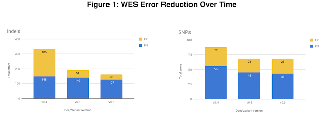
In v0.5 we also focused on exome data, which is the subset of the genome that directly codes for proteins. The exome is only ~1% of the whole human genome, so whole exome sequencing (WES) costs less than whole genome sequencing (WGS). The exome also harbors many variants of clinical significance which makes it useful for both researchers and clinicians. To increase exome accuracy we added a variety of WES datatypes, provided by DNAnexus, to DeepVariant's training data. The v0.5 WES model shows 43% fewer indel (insertion-deletion) errors and a 22% reduction in single nucleotide polymorphism (SNP) errors.
The total number of exome errors for HG002 across DeepVariant versions, broken down by indel errors (left) and SNP errors (right). Errors are either false positive (FP), colored yellow, or false negative (FN), colored blue. The largest accuracy jump is between v0.4 and v0.5, largely attributable to a reduction in indel FPs.
Improved Whole Genome Sequencing Model for PCR+ data in v0.6
Our newest release of DeepVariant, v0.6, focuses on improved accuracy for data that has undergone DNA amplification via polymerase chain reaction (PCR) prior to sequencing. PCR is an easy and inexpensive way to amplify very small quantities of DNA, and once sequenced results in what is known as PCR positive (PCR+) sequencing data. It is well known, however, that PCR can be prone to bias and errors, and non-PCR-based (or PCR-free) DNA preparation methods are increasingly common. DeepVariant's training data prior to the v0.6 release was exclusively PCR-free data, and PCR+ was one of the few datatypes for which DeepVariant had underperformed in external evaluations. By adding PCR+ examples to DeepVariant's training data, also provided by DNAnexus, we have seen significant accuracy improvements for this datatype, including a 60% reduction in indel errors.
DeepVariant v0.6 shows major accuracy improvements for PCR+ data, largely attributable to a reduction in indel errors. Here we re-analyze two PCR+ samples that were used in external evaluations, including DNAnexus on the left (see details in figure 10) and bcbio on the right, showing how indel accuracy improves with each DeepVariant version.
Independent evaluations of DeepVariant v0.6 from both DNAnexus and bcbio are also available. Their analyses support our findings of improved indel accuracy, and also include comparisons to other variant calling tools.

Looking Forward
We released DeepVariant as open source software to encourage collaboration and to accelerate the use of this technology to solve real world problems. As the pace of innovation in sequencing technologies continues to grow, including more clinical applications, we are optimistic that DeepVariant can be further extended to produce consistent and highly accurate results. We hope that researchers will use DeepVariant v0.6 to accelerate discoveries, and if there is a sequencing datatype that you would like to see us prioritize, please let us know.
Source: Google AI Blog


An Augmented Reality Microscope for Cancer Detection


Applications of deep learning to medical disciplines including ophthalmology, dermatology, radiology, and pathology have recently shown great promise to increase both the accuracy and availability of high-quality healthcare to patients around the world. At Google, we have also published results showing that a convolutional neural network is able to detect breast cancer metastases in lymph nodes at a level of accuracy comparable to a trained pathologist. However, because direct tissue visualization using a compound light microscope remains the predominant means by which a pathologist diagnoses illness, a critical barrier to the widespread adoption of deep learning in pathology is the dependence on having a digital representation of the microscopic tissue.

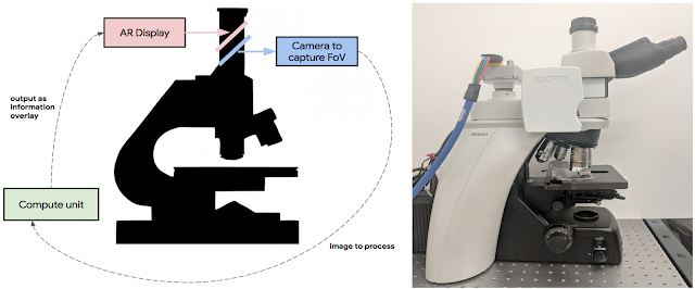
Today, in a talk delivered at the Annual Meeting of the American Association for Cancer Research (AACR), with an accompanying paper “An Augmented Reality Microscope for Real-time Automated Detection of Cancer” (under review), we describe a prototype Augmented Reality Microscope (ARM) platform that we believe can possibly help accelerate and democratize the adoption of deep learning tools for pathologists around the world. The platform consists of a modified light microscope that enables real-time image analysis and presentation of the results of machine learning algorithms directly into the field of view. Importantly, the ARM can be retrofitted into existing light microscopes found in hospitals and clinics around the world using low-cost, readily-available components, and without the need for whole slide digital versions of the tissue being analyzed.
Modern computational components and deep learning models, such as those built upon TensorFlow, will allow a wide range of pre-trained models to run on this platform. As in a traditional analog microscope, the user views the sample through the eyepiece. A machine learning algorithm projects its output back into the optical path in real-time. This digital projection is visually superimposed on the original (analog) image of the specimen to assist the viewer in localizing or quantifying features of interest. Importantly, the computation and visual feedback updates quickly — our present implementation runs at approximately 10 frames per second, so the model output updates seamlessly as the user scans the tissue by moving the slide and/or changing magnification.
Left: Schematic overview of the ARM. A digital camera captures the same field of view (FoV) as the user and passes the image to an attached compute unit capable of running real-time inference of a machine learning model. The results are fed back into a custom AR display which is inline with the ocular lens and projects the model output on the same plane as the slide. Right: A picture of our prototype which has been retrofitted into a typical clinical-grade light microscope.
In principle, the ARM can provide a wide variety of visual feedback, including text, arrows, contours, heatmaps, or animations, and is capable of running many types of machine learning algorithms aimed at solving different problems such as object detection, quantification, or classification.

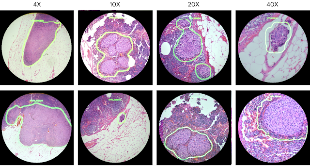
As a demonstration of the potential utility of the ARM, we configured it to run two different cancer detection algorithms: one that detects breast cancer metastases in lymph node specimens, and another that detects prostate cancer in prostatectomy specimens. These models can run at magnifications between 4-40x, and the result of a given model is displayed by outlining detected tumor regions with a green contour. These contours help draw the pathologist’s attention to areas of interest without obscuring the underlying tumor cell appearance.
Example view through the lens of the ARM. These images show examples of the lymph node metastasis model with 4x, 10x, 20x, and 40x microscope objectives.
While both cancer models were originally trained on images from a whole slide scanner with a significantly different optical configuration, the models performed remarkably well on the ARM with no additional re-training. For example, the lymph node metastasis model had an area-under-the-curve (AUC) of 0.98 and our prostate cancer model had an AUC of 0.96 for cancer detection in the field of view (FoV) when run on the ARM, only slightly decreased performance than obtained on WSI. We believe it is likely that the performance of these models can be further improved by additional training on digital images captured directly from the ARM itself.

We believe that the ARM has potential for a large impact on global health, particularly for the diagnosis of infectious diseases, including tuberculosis and malaria, in developing countries. Furthermore, even in hospitals that will adopt a digital pathology workflow in the near future, ARM could be used in combination with the digital workflow where scanners still face major challenges or where rapid turnaround is required (e.g. cytology, fluorescent imaging, or intra-operative frozen sections). Of course, light microscopes have proven useful in many industries other than pathology, and we believe the ARM can be adapted for a broad range of applications across healthcare, life sciences research, and material science. We’re excited to continue to explore how the ARM can help accelerate the adoption of machine learning for positive impact around the world.


Source: Google AI Blog


Using Machine Learning to Discover Neural Network Optimizers


Deep learning models have been deployed in numerous Google products, such as Search, Translate and Photos. The choice of optimization method plays a major role when training deep learning models. For example, stochastic gradient descent works well in many situations, but more advanced optimizers can be faster, especially for training very deep networks. Coming up with new optimizers for neural networks, however, is challenging due to to the non-convex nature of the optimization problem. On the Google Brain team, we wanted to see if it could be possible to automate the discovery of new optimizers, in a way that is similar to how AutoML has been used to discover new competitive neural network architectures.

In “Neural Optimizer Search with Reinforcement Learning”, we present a method to discover optimization methods with a focus on deep learning architectures. Using this method we found two new optimizers, PowerSign and AddSign, that are competitive on a variety of different tasks and architectures, including ImageNet classification and Google’s neural machine translation system. To help others benefit from this work we have made the optimizers available in Tensorflow.

Neural Optimizer Search makes use of a recurrent neural network controller which is given access to a list of simple primitives that are typically relevant for optimization. These primitives include, for example, the gradient or the running average of the gradient and lead to search spaces with over 1010 possible combinations. The controller then generates the computation graph for a candidate optimizer or update rule in that search space.

In our paper, proposed candidate update rules (U) are used to train a child convolutional neural network on CIFAR10 for a few epochs and the final validation accuracy (R) is fed as a reward to the controller. The controller is trained with reinforcement learning to maximize the validation accuracies of the sampled update rules. This process is illustrated below.
An overview of Neural Optimizer Search using an iterative process to discover new optimizers.
Interestingly, the optimizers we have found are interpretable. For example, in the PowerSign optimizer we are releasing, each update compares the sign of the gradient and its running average, adjusting the step size according to whether those two values agree. The intuition behind this is that if these values agree, one is more confident in the direction of the update, and thus the step size can be larger. We also discovered a simple learning rate decay scheme, linear cosine decay, which we found can lead to faster convergence.
Graph comparing learning rate decay functions for linear cosine decay, stepwise decay and cosine decay.
Neural Optimizer Search found several optimizers that outperform commonly used optimizers on the small ConvNet model. Among the ones that transfer well to other tasks, we found that PowerSign and AddSign improve top-1 and top-5 accuracy of a state-of-the-art ImageNet mobile-sized model by up to 0.4%. They also work well on Google’s Neural Machine Translation system, giving an improvement of up to 0.7 using bilingual evaluation metrics (BLEU) on an English to German translation task.

We are excited that Neural Optimizer Search can not only improve the performance of machine learning models but also potentially lead to new, interpretable equations and discoveries. It is our hope that open sourcing these optimizers in Tensorflow will be useful to machine learning practitioners.

Source: Google AI Blog


Using Evolutionary AutoML to Discover Neural Network Architectures


The brain has evolved over a long time, from very simple worm brains 500 million years ago to a diversity of modern structures today. The human brain, for example, can accomplish a wide variety of activities, many of them effortlessly — telling whether a visual scene contains animals or buildings feels trivial to us, for example. To perform activities like these, artificial neural networks require careful design by experts over years of difficult research, and typically address one specific task, such as to find what's in a photograph, to call a genetic variant, or to help diagnose a disease. Ideally, one would want to have an automated method to generate the right architecture for any given task.

One approach to generate these architectures is through the use of evolutionary algorithms. Traditional research into neuro-evolution of topologies (e.g. Stanley and Miikkulainen 2002) has laid the foundations that allow us to apply these algorithms at scale today, and many groups are working on the subject, including OpenAI, Uber Labs, Sentient Labs and DeepMind. Of course, the Google Brain team has been thinking about AutoML too. In addition to learning-based approaches (eg. reinforcement learning), we wondered if we could use our computational resources to programmatically evolve image classifiers at unprecedented scale. Can we achieve solutions with minimal expert participation? How good can today's artificially-evolved neural networks be? We address these questions through two papers.

In “Large-Scale Evolution of Image Classifiers,” presented at ICML 2017, we set up an evolutionary process with simple building blocks and trivial initial conditions. The idea was to "sit back" and let evolution at scale do the work of constructing the architecture. Starting from very simple networks, the process found classifiers comparable to hand-designed models at the time. This was encouraging because many applications may require little user participation. For example, some users may need a better model but may not have the time to become machine learning experts. A natural question to consider next was whether a combination of hand-design and evolution could do better than either approach alone. Thus, in our more recent paper, “Regularized Evolution for Image Classifier Architecture Search” (2018), we participated in the process by providing sophisticated building blocks and good initial conditions (discussed below). Moreover, we scaled up computation using Google's new TPUv2 chips. This combination of modern hardware, expert knowledge, and evolution worked together to produce state-of-the-art models on CIFAR-10 and ImageNet, two popular benchmarks for image classification.

A Simple Approach
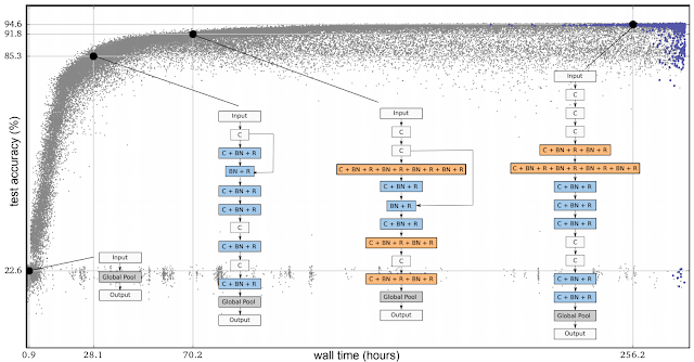
The following is an example of an experiment from our first paper. In the figure below, each dot is a neural network trained on the CIFAR-10 dataset, which is commonly used to train image classifiers. Initially, the population consists of one thousand identical simple seed models (no hidden layers). Starting from simple seed models is important — if we had started from a high-quality model with initial conditions containing expert knowledge, it would have been easier to get a high-quality model in the end. Once seeded with the simple models, the process advances in steps. At each step, a pair of neural networks is chosen at random. The network with higher accuracy is selected as a parent and is copied and mutated to generate a child that is then added to the population, while the other neural network dies out. All other networks remain unchanged during the step. With the application of many such steps in succession, the population evolves.
Progress of an evolution experiment. Each dot represents an individual in the population. The four diagrams show examples of discovered architectures. These correspond to the best individual (rightmost; selected by validation accuracy) and three of its ancestors.
The mutations in our first paper are purposefully simple: remove a convolution at random, add a skip connection between arbitrary layers, or change the learning rate, to name a few. This way, the results show the potential of the evolutionary algorithm, as opposed to the quality of the search space. For example, if we had used a single mutation that transforms one of the seed networks into an Inception-ResNet classifier in one step, we would be incorrectly concluding that the algorithm found a good answer. Yet, in that case, all we would have done is hard-coded the final answer into a complex mutation, rigging the outcome. If instead we stick with simple mutations, this cannot happen and evolution is truly doing the job. In the experiment in the figure, simple mutations and the selection process cause the networks to improve over time and reach high test accuracies, even though the test set had never been seen during the process. In this paper, the networks can also inherit their parent's weights. Thus, in addition to evolving the architecture, the population trains its networks while exploring the search space of initial conditions and learning-rate schedules. As a result, the process yields fully trained models with optimized hyperparameters. No expert input is needed after the experiment starts.

In all the above, even though we were minimizing the researcher's participation by having simple initial architectures and intuitive mutations, a good amount of expert knowledge went into the building blocks those architectures were made of. These included important inventions such as convolutions, ReLUs and batch-normalization layers. We were evolving an architecture made up of these components. The term "architecture" is not accidental: this is analogous to constructing a house with high-quality bricks.

Combining Evolution and Hand Design
After our first paper, we wanted to reduce the search space to something more manageable by giving the algorithm fewer choices to explore. Using our architectural analogy, we removed all the possible ways of making large-scale errors, such as putting the wall above the roof, from the search space. Similarly with neural network architecture searches, by fixing the large-scale structure of the network, we can help the algorithm out. So how to do this? The inception-like modules introduced in Zoph et al. (2017) for the purpose of architecture search proved very powerful. Their idea is to have a deep stack of repeated modules called cells. The stack is fixed but the architecture of the individual modules can change.
The building blocks introduced in Zoph et al. (2017). The diagram on the left is the outer structure of the full neural network, which parses the input data from bottom to top through a stack of repeated cells. The diagram on the right is the inside structure of a cell. The goal is to find a cell that yields an accurate network.
In our second paper, “Regularized Evolution for Image Classifier Architecture Search” (2018), we presented the results of applying evolutionary algorithms to the search space described above. The mutations modify the cell by randomly reconnecting the inputs (the arrows on the right diagram in the figure) or randomly replacing the operations (for example, they can replace the "max 3x3" in the figure, a max-pool operation, with an arbitrary alternative). These mutations are still relatively simple, but the initial conditions are not: the population is now initialized with models that must conform to the outer stack of cells, which was designed by an expert. Even though the cells in these seed models are random, we are no longer starting from simple models, which makes it easier to get to high-quality models in the end. If the evolutionary algorithm is contributing meaningfully, the final networks should be significantly better than the networks we already know can be constructed within this search space. Our paper shows that evolution can indeed find state-of-the-art models that either match or outperform hand-designs.

A Controlled Comparison
Even though the mutation/selection evolutionary process is not complicated, maybe an even more straightforward approach (like random search) could have done the same. Other alternatives, though not simpler, also exist in the literature (like reinforcement learning). Because of this, the main purpose of our second paper was to provide a controlled comparison between techniques.
Comparison between evolution, reinforcement learning, and random search for the purposes of architecture search. These experiments were done on the CIFAR-10 dataset, under the same conditions as Zoph et al. (2017), where the search space was originally used with reinforcement learning.
The figure above compares evolution, reinforcement learning, and random search. On the left, each curve represents the progress of an experiment, showing that evolution is faster than reinforcement learning in the earlier stages of the search. This is significant because with less compute power available, the experiments may have to stop early. Moreover evolution is quite robust to changes in the dataset or search space. Overall, the goal of this controlled comparison is to provide the research community with the results of a computationally expensive experiment. In doing so, it is our hope to facilitate architecture searches for everyone by providing a case study of the relationship between the different search algorithms. Note, for example, that the figure above shows that the final models obtained with evolution can reach very high accuracy while using fewer floating-point operations.

One important feature of the evolutionary algorithm we used in our second paper is a form of regularization: instead of letting the worst neural networks die, we remove the oldest ones — regardless of how good they are. This improves robustness to changes in the task being optimized and tends to produce more accurate networks in the end. One reason for this may be that since we didn't allow weight inheritance, all networks must train from scratch. Therefore, this form of regularization selects for networks that remain good when they are re-trained. In other words, because a model can be more accurate just by chance — noise in the training process means even identical architectures may get different accuracy values — only architectures that remain accurate through the generations will survive in the long run, leading to the selection of networks that retrain well. More details of this conjecture can be found in the paper.

The state-of-the-art models we evolved are nicknamed AmoebaNets, and are one of the latest results from our AutoML efforts. All these experiments took a lot of computation — we used hundreds of GPUs/TPUs for days. Much like a single modern computer can outperform thousands of decades-old machines, we hope that in the future these experiments will become household. Here we aimed to provide a glimpse into that future.

Acknowledgements
We would like to thank Alok Aggarwal, Yanping Huang, Andrew Selle, Sherry Moore, Saurabh Saxena, Yutaka Leon Suematsu, Jie Tan, Alex Kurakin, Quoc Le, Barret Zoph, Jon Shlens, Vijay Vasudevan, Vincent Vanhoucke, Megan Kacholia, Jeff Dean, and the rest of the Google Brain team for the collaborations that made this work possible.

Source: Google AI Blog


Open Sourcing the Hunt for Exoplanets


Recently, we discovered two exoplanets by training a neural network to analyze data from NASA’s Kepler space telescope and accurately identify the most promising planet signals. And while this was only an initial analysis of ~700 stars, we consider this a successful proof-of-concept for using machine learning to discover exoplanets, and more generally another example of using machine learning to make meaningful gains in a variety of scientific disciplines (e.g. healthcare, quantum chemistry, and fusion research).

Today, we’re excited to release our code for processing the Kepler data, training our neural network model, and making predictions about new candidate signals. We hope this release will prove a useful starting point for developing similar models for other NASA missions, like K2 (Kepler’s second mission) and the upcoming Transiting Exoplanet Survey Satellite mission. As well as announcing the release of our code, we’d also like take this opportunity to dig a bit deeper into how our model works.

A Planet Hunting Primer

First, let’s consider how data collected by the Kepler telescope is used to detect the presence of a planet. The plot below is called a light curve, and it shows the brightness of the star (as measured by Kepler’s photometer) over time. When a planet passes in front of the star, it temporarily blocks some of the light, which causes the measured brightness to decrease and then increase again shortly thereafter, causing a “U-shaped” dip in the light curve.
A light curve from the Kepler space telescope with a “U-shaped” dip that indicates a transiting exoplanet.
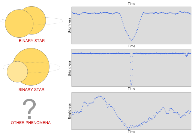
However, other astronomical and instrumental phenomena can also cause the measured brightness of a star to decrease, including binary star systems, starspots, cosmic ray hits on Kepler’s photometer, and instrumental noise.
The first light curve has a “V-shaped” pattern that tells us that a very large object (i.e. another star) passed in front of the star that Kepler was observing. The second light curve contains two places where the brightness decreases, which indicates a binary system with one bright and one dim star: the larger dip is caused by the dimmer star passing in front of the brighter star, and vice versa. The third light curve is one example of the many other non-planet signals where the measured brightness of a star appears to decrease.
To search for planets in Kepler data, scientists use automated software (e.g. the Kepler data processing pipeline) to detect signals that might be caused by planets, and then manually follow up to decide whether each signal is a planet or a false positive. To avoid being overwhelmed with more signals than they can manage, the scientists apply a cutoff to the automated detections: those with signal-to-noise ratios above a fixed threshold are deemed worthy of follow-up analysis, while all detections below the threshold are discarded. Even with this cutoff, the number of detections is still formidable: to date, over 30,000 detected Kepler signals have been manually examined, and about 2,500 of those have been validated as actual planets!

Perhaps you’re wondering: does the signal-to-noise cutoff cause some real planet signals to be missed? The answer is, yes! However, if astronomers need to manually follow up on every detection, it’s not really worthwhile to lower the threshold, because as the threshold decreases the rate of false positive detections increases rapidly and actual planet detections become increasingly rare. However, there’s a tantalizing incentive: it’s possible that some potentially habitable planets like Earth, which are relatively small and orbit around relatively dim stars, might be hiding just below the traditional detection threshold — there might be hidden gems still undiscovered in the Kepler data!

A Machine Learning Approach

The Google Brain team applies machine learning to a diverse variety of data, from human genomes to sketches to formal mathematical logic. Considering the massive amount of data collected by the Kepler telescope, we wondered what we might find if we used machine learning to analyze some of the previously unexplored Kepler data. To find out, we teamed up with Andrew Vanderburg at UT Austin and developed a neural network to help search the low signal-to-noise detections for planets.
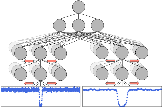
We trained a convolutional neural network (CNN) to predict the probability that a given Kepler signal is caused by a planet. We chose a CNN because they have been very successful in other problems with spatial and/or temporal structure, like audio generation and image classification.
Luckily, we had 30,000 Kepler signals that had already been manually examined and classified by humans. We used a subset of around 15,000 of these signals, of which around 3,500 were verified planets or strong planet candidates, to train our neural network to distinguish planets from false positives. The inputs to our network are two separate views of the same light curve: a wide view that allows the model to examine signals elsewhere on the light curve (e.g., a secondary signal caused by a binary star), and a zoomed-in view that enables the model to closely examine the shape of the detected signal (e.g., to distinguish “U-shaped” signals from “V-shaped” signals).

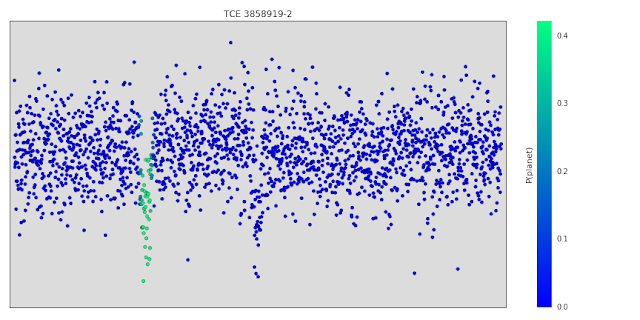
Once we had trained our model, we investigated the features it learned about light curves to see if they matched with our expectations. One technique we used (originally suggested in this paper) was to systematically occlude small regions of the input light curves to see whether the model’s output changed. Regions that are particularly important to the model’s decision will change the output prediction if they are occluded, but occluding unimportant regions will not have a significant effect. Below is a light curve from a binary star that our model correctly predicts is not a planet. The points highlighted in green are the points that most change the model’s output prediction when occluded, and they correspond exactly to the secondary “dip” indicative of a binary system. When those points are occluded, the model’s output prediction changes from ~0% probability of being a planet to ~40% probability of being a planet. So, those points are part of the reason the model rejects this light curve, but the model uses other evidence as well - for example, zooming in on the centred primary dip shows that it's actually “V-shaped”, which is also indicative of a binary system.

Searching for New Planets

Once we were confident with our model’s predictions, we tested its effectiveness by searching for new planets in a small set 670 stars. We chose these stars because they were already known to have multiple orbiting planets, and we believed that some of these stars might host additional planets that had not yet been detected. Importantly, we allowed our search to include signals that were below the signal-to-noise threshold that astronomers had previously considered. As expected, our neural network rejected most of these signals as spurious detections, but a handful of promising candidates rose to the top, including our two newly discovered planets: Kepler-90 i and Kepler-80 g.

Find your own Planet(s)!

Let’s take a look at how the code released today can help (re-)discover the planet Kepler-90 i. The first step is to train a model by following the instructions on the code’s home page. It takes a while to download and process the data from the Kepler telescope, but once that’s done, it’s relatively fast to train a model and make predictions about new signals. One way to find new signals to show the model is to use an algorithm called Box Least Squares (BLS), which searches for periodic “box shaped” dips in brightness (see below). The BLS algorithm will detect “U-shaped” planet signals, “V-shaped” binary star signals and many other types of false positive signals to show the model. There are various freely available software implementations of the BLS algorithm, including VARTOOLS and LcTools. Alternatively, you can even look for candidate planet transits by eye, like the Planet Hunters.
A low signal-to-noise detection in the light curve of the Kepler 90 star detected by the BLS algorithm. The detection has period 14.44912 days, duration 2.70408 hours (0.11267 days) beginning 2.2 days after 12:00 on 1/1/2009 (the year the Kepler telescope launched).
To run this detected signal though our trained model, we simply execute the following command:
python predict.py  --kepler_id=11442793 --period=14.44912 --t0=2.2
--duration=0.11267 --kepler_data_dir=$HOME/astronet/kepler
--output_image_file=$HOME/astronet/kepler-90i.png
--model_dir=$HOME/astronet/model
The output of the command is prediction = 0.94, which means the model is 94% certain that this signal is a real planet. Of course, this is only a small step in the overall process of discovering and validating an exoplanet: the model’s prediction is not proof one way or the other. The process of validating this signal as a real exoplanet requires significant follow-up work by an expert astronomer — see Sections 6.3 and 6.4 of our paper for the full details. In this particular case, our follow-up analysis validated this signal as a bona fide exoplanet, and it’s now called Kepler-90 i!
Our work here is far from done. We’ve only searched 670 stars out of 200,000 observed by Kepler — who knows what we might find when we turn our technique to the entire dataset. Before we do that, though, we have a few improvements we want to make to our model. As we discussed in our paper, our model is not yet as good at rejecting binary stars and instrumental false positives as some more mature computer heuristics. We’re hard at work improving our model, and now that it’s open sourced, we hope others will do the same!


By Chris Shallue, Senior Software Engineer, Google Brain Team

If you’d like to learn more, Chris is featured on the latest episode of This Week In Machine Learning discussing his work.

Open Sourcing the Hunt for Exoplanets


Recently, we discovered two exoplanets by training a neural network to analyze data from NASA’s Kepler space telescope and accurately identify the most promising planet signals. And while this was only an initial analysis of ~700 stars, we consider this a successful proof-of-concept for using machine learning to discover exoplanets, and more generally another example of using machine learning to make meaningful gains in a variety of scientific disciplines (e.g. healthcare, quantum chemistry, and fusion research).

Today, we’re excited to release our code for processing the Kepler data, training our neural network model, and making predictions about new candidate signals. We hope this release will prove a useful starting point for developing similar models for other NASA missions, like K2 (Kepler’s second mission) and the upcoming Transiting Exoplanet Survey Satellite mission. As well as announcing the release of our code, we’d also like take this opportunity to dig a bit deeper into how our model works.

A Planet Hunting Primer
First, let’s consider how data collected by the Kepler telescope is used to detect the presence of a planet. The plot below is called a light curve, and it shows the brightness of the star (as measured by Kepler’s photometer) over time. When a planet passes in front of the star, it temporarily blocks some of the light, which causes the measured brightness to decrease and then increase again shortly thereafter, causing a “U-shaped” dip in the light curve.
A light curve from the Kepler space telescope with a “U-shaped” dip that indicates a transiting exoplanet.
However, other astronomical and instrumental phenomena can also cause the measured brightness of a star to decrease, including binary star systems, starspots, cosmic ray hits on Kepler’s photometer, and instrumental noise.
The first light curve has a “V-shaped” pattern that tells us that a very large object (i.e. another star) passed in front of the star that Kepler was observing. The second light curve contains two places where the brightness decreases, which indicates a binary system with one bright and one dim star: the larger dip is caused by the dimmer star passing in front of the brighter star, and vice versa. The third light curve is one example of the many other non-planet signals where the measured brightness of a star appears to decrease.
To search for planets in Kepler data, scientists use automated software (e.g. the Kepler data processing pipeline) to detect signals that might be caused by planets, and then manually follow up to decide whether each signal is a planet or a false positive. To avoid being overwhelmed with more signals than they can manage, the scientists apply a cutoff to the automated detections: those with signal-to-noise ratios above a fixed threshold are deemed worthy of follow-up analysis, while all detections below the threshold are discarded. Even with this cutoff, the number of detections is still formidable: to date, over 30,000 detected Kepler signals have been manually examined, and about 2,500 of those have been validated as actual planets!

Perhaps you’re wondering: does the signal-to-noise cutoff cause some real planet signals to be missed? The answer is, yes! However, if astronomers need to manually follow up on every detection, it’s not really worthwhile to lower the threshold, because as the threshold decreases the rate of false positive detections increases rapidly and actual planet detections become increasingly rare. However, there’s a tantalizing incentive: it’s possible that some potentially habitable planets like Earth, which are relatively small and orbit around relatively dim stars, might be hiding just below the traditional detection threshold — there might be hidden gems still undiscovered in the Kepler data!

A Machine Learning Approach
The Google Brain team applies machine learning to a diverse variety of data, from human genomes to sketches to formal mathematical logic. Considering the massive amount of data collected by the Kepler telescope, we wondered what we might find if we used machine learning to analyze some of the previously unexplored Kepler data. To find out, we teamed up with Andrew Vanderburg at UT Austin and developed a neural network to help search the low signal-to-noise detections for planets.
We trained a convolutional neural network (CNN) to predict the probability that a given Kepler signal is caused by a planet. We chose a CNN because they have been very successful in other problems with spatial and/or temporal structure, like audio generation and image classification.
Luckily, we had 30,000 Kepler signals that had already been manually examined and classified by humans. We used a subset of around 15,000 of these signals, of which around 3,500 were verified planets or strong planet candidates, to train our neural network to distinguish planets from false positives. The inputs to our network are two separate views of the same light curve: a wide view that allows the model to examine signals elsewhere on the light curve (e.g., a secondary signal caused by a binary star), and a zoomed-in view that enables the model to closely examine the shape of the detected signal (e.g., to distinguish “U-shaped” signals from “V-shaped” signals).

Once we had trained our model, we investigated the features it learned about light curves to see if they matched with our expectations. One technique we used (originally suggested in this paper) was to systematically occlude small regions of the input light curves to see whether the model’s output changed. Regions that are particularly important to the model’s decision will change the output prediction if they are occluded, but occluding unimportant regions will not have a significant effect. Below is a light curve from a binary star that our model correctly predicts is not a planet. The points highlighted in green are the points that most change the model’s output prediction when occluded, and they correspond exactly to the secondary “dip” indicative of a binary system. When those points are occluded, the model’s output prediction changes from ~0% probability of being a planet to ~40% probability of being a planet. So, those points are part of the reason the model rejects this light curve, but the model uses other evidence as well - for example, zooming in on the centred primary dip shows that it's actually “V-shaped”, which is also indicative of a binary system.
Searching for New Planets
Once we were confident with our model’s predictions, we tested its effectiveness by searching for new planets in a small set 670 stars. We chose these stars because they were already known to have multiple orbiting planets, and we believed that some of these stars might host additional planets that had not yet been detected. Importantly, we allowed our search to include signals that were below the signal-to-noise threshold that astronomers had previously considered. As expected, our neural network rejected most of these signals as spurious detections, but a handful of promising candidates rose to the top, including our two newly discovered planets: Kepler-90 i and Kepler-80 g.

Find your own Planet(s)!
Let’s take a look at how the code released today can help (re-)discover the planet Kepler-90 i. The first step is to train a model by following the instructions on the code’s home page. It takes a while to download and process the data from the Kepler telescope, but once that’s done, it’s relatively fast to train a model and make predictions about new signals. One way to find new signals to show the model is to use an algorithm called Box Least Squares (BLS), which searches for periodic “box shaped” dips in brightness (see below). The BLS algorithm will detect “U-shaped” planet signals, “V-shaped” binary star signals and many other types of false positive signals to show the model. There are various freely available software implementations of the BLS algorithm, including VARTOOLS and LcTools. Alternatively, you can even look for candidate planet transits by eye, like the Planet Hunters.
A low signal-to-noise detection in the light curve of the Kepler 90 star detected by the BLS algorithm. The detection has period 14.44912 days, duration 2.70408 hours (0.11267 days) beginning 2.2 days after 12:00 on 1/1/2009 (the year the Kepler telescope launched).
To run this detected signal though our trained model, we simply execute the following command:
python predict.py  --kepler_id=11442793 --period=14.44912 --t0=2.2
--duration=0.11267 --kepler_data_dir=$HOME/astronet/kepler
--output_image_file=$HOME/astronet/kepler-90i.png
--model_dir=$HOME/astronet/model
The output of the command is prediction = 0.94, which means the model is 94% certain that this signal is a real planet. Of course, this is only a small step in the overall process of discovering and validating an exoplanet: the model’s prediction is not proof one way or the other. The process of validating this signal as a real exoplanet requires significant follow-up work by an expert astronomer — see Sections 6.3 and 6.4 of our paper for the full details. In this particular case, our follow-up analysis validated this signal as a bona fide exoplanet, and it’s now called Kepler-90 i!
Our work here is far from done. We’ve only searched 670 stars out of 200,000 observed by Kepler — who knows what we might find when we turn our technique to the entire dataset. Before we do that, though, we have a few improvements we want to make to our model. As we discussed in our paper, our model is not yet as good at rejecting binary stars and instrumental false positives as some more mature computer heuristics. We’re hard at work improving our model, and now that it’s open sourced, we hope others will do the same!

If you’d like to learn more, Chris is featured on the latest episode of This Week In Machine Learning & AI discussing his work.

The Building Blocks of Interpretability

Cross-posted on the Google Research Blog.

In 2015, our early attempts to visualize how neural networks understand images led to psychedelic images. Soon after, we open sourced our code as DeepDream and it grew into a small art movement producing all sorts of amazing things. But we also continued the original line of research behind DeepDream, trying to address one of the most exciting questions in Deep Learning: how do neural networks do what they do?

Last year in the online journal Distill, we demonstrated how those same techniques could show what individual neurons in a network do, rather than just what is “interesting to the network” as in DeepDream. This allowed us to see how neurons in the middle of the network are detectors for all sorts of things — buttons, patches of cloth, buildings — and see how those build up to be more and more sophisticated over the networks layers.
Visualizations of neurons in GoogLeNet. Neurons in higher layers represent higher level ideas.
While visualizing neurons is exciting, our work last year was missing something important: how do these neurons actually connect to what the network does in practice?

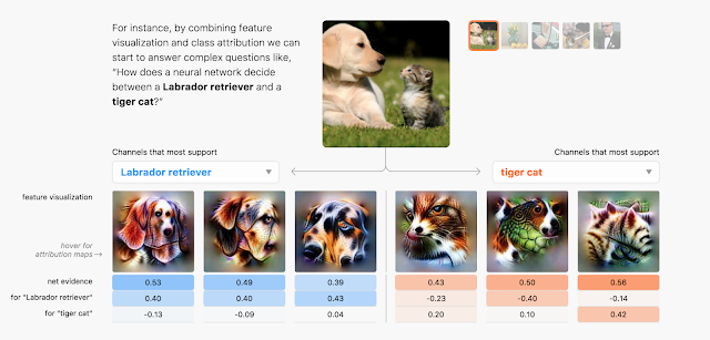
Today, we’re excited to publish “The Building Blocks of Interpretability,” a new Distill article exploring how feature visualization can combine together with other interpretability techniques to understand aspects of how networks make decisions. We show that these combinations can allow us to sort of “stand in the middle of a neural network” and see some of the decisions being made at that point, and how they influence the final output. For example, we can see things like how a network detects a floppy ear, and then that increases the probability it gives to the image being a “Labrador retriever” or “beagle”.

We explore techniques for understanding which neurons fire in the network. Normally, if we ask which neurons fire, we get something meaningless like “neuron 538 fired a little bit,” which isn’t very helpful even to experts. Our techniques make things more meaningful to humans by attaching visualizations to each neuron, so we can see things like “the floppy ear detector fired”. It’s almost a kind of MRI for neural networks.
We can also zoom out and show how the entire image was “perceived” at different layers. This allows us to really see the transition from the network detecting very simple combinations of edges, to rich textures and 3d structure, to high-level structures like ears, snouts, heads and legs.
These insights are exciting by themselves, but they become even more exciting when we can relate them to the final decision the network makes. So not only can we see that the network detected a floppy ear, but we can also see how that increases the probability of the image being a labrador retriever.
In addition to our paper, we’re also releasing Lucid, a neural network visualization library building off our work on DeepDream. It allows you to make the sort lucid feature visualizations we see above, in addition to more artistic DeepDream images.

We’re also releasing colab notebooks. These notebooks make it extremely easy to use Lucid to reproduce visualizations in our article! Just open the notebook, click a button to run code — no setup required!
In colab notebooks you can click a button to run code, and see the result below.
This work only scratches the surface of the kind of interfaces that we think it’s possible to build for understanding neural networks. We’re excited to see what the community will do — and we’re excited to work together towards deeper human understanding of neural networks.

By Chris Olah, Research Scientist and Arvind Satyanarayan, Visiting Researcher, Google Brain Team