Tag Archives: deep learning

Advancing NLP with Efficient Projection-Based Model Architectures

Deep neural networks have radically transformed natural language processing (NLP) in the last decade, primarily through their application in data centers using specialized hardware. However, issues such as preserving user privacy, eliminating network latency, enabling offline functionality, and reducing operation costs have rapidly spurred the development of NLP models that can be run on-device rather than in data centers. Yet mobile devices have limited memory and processing power, which requires models running on them to be small and efficient — without compromising quality.

Last year, we published a neural architecture called PRADO, which at the time achieved state-of-the-art performance on many text classification problems, using a model with less than 200K parameters. While most models use a fixed number of parameters per token, the PRADO model used a network structure that required extremely few parameters to learn the most relevant or useful tokens for the task.

Today we describe a new extension to the model, called pQRNN, which advances the state of the art for NLP performance with a minimal model size. The novelty of pQRNN is in how it combines a simple projection operation with a quasi-RNN encoder for fast, parallel processing. We show that the pQRNN model is able to achieve BERT-level performance on a text classification task with orders of magnitude fewer number of parameters.

What Makes PRADO Work?
When developed a year ago, PRADO exploited NLP domain-specific knowledge on text segmentation to reduce the model size and improve the performance. Normally, the text input to NLP models is first processed into a form that is suitable for the neural network, by segmenting text into pieces (tokens) that correspond to values in a predefined universal dictionary (a list of all possible tokens). The neural network then uniquely identifies each segment using a trainable parameter vector, which comprises the embedding table. However, the way in which text is segmented has a significant impact on the model performance, size, and latency. The figure below shows the spectrum of approaches used by the NLP community and their pros and cons.

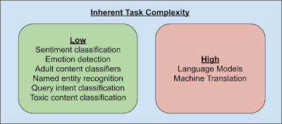
Since the number of text segments is such an important parameter for model performance and compression, it raises the question of whether or not an NLP model needs to be able to distinctly identify every possible text segment. To answer this question we look at the inherent complexity of NLP tasks.

Only a few NLP tasks (e.g., language models and machine translation) need to know subtle differences between text segments and thus need to be capable of uniquely identifying all possible text segments. In contrast, the majority of other tasks can be solved by knowing a small subset of these segments. Furthermore, this subset of task-relevant segments will likely not be the most frequent, as a significant fraction of segments will undoubtedly be dedicated to articles, such as a, an, the, etc., which for many tasks are not necessarily critical. Hence, allowing the network to determine the most relevant segments for a given task results in better performance. In addition, the network does not need to be able to uniquely identify these segments, but only needs to recognize clusters of text segments. For example, a sentiment classifier just needs to know segment clusters that are strongly correlated to the sentiment in the text.

Leveraging these insights, PRADO was designed to learn clusters of text segments from words rather than word pieces or characters, which enabled it to achieve good performance on low-complexity NLP tasks. Since word units are more meaningful, and yet the most relevant words for most tasks are reasonably small, many fewer model parameters are needed to learn such a reduced subset of relevant word clusters.

Improving PRADO
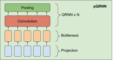
Building on the success of PRADO, we developed an improved NLP model, called pQRNN. This model is composed of three building blocks, a projection operator that converts tokens in text to a sequence of ternary vectors, a dense bottleneck layer and a stack of QRNN encoders.

The implementation of the projection layer in pQRNN is identical to that used in PRADO and helps the model learn the most relevant tokens without a fixed set of parameters to define them. It first fingerprints the tokens in the text and converts it to a ternary feature vector using a simple mapping function. This results in a ternary vector sequence with a balanced symmetric distribution that uniquely represents the text. This representation is not directly useful since it does not have any information needed to solve the task of interest and the network has no control over this representation. We combine it with a dense bottleneck layer to allow the network to learn a per word representation that is relevant for the task at hand. The representation resulting from the bottleneck layer still does not take the context of the word into account. We learn a contextual representation by using a stack of bidirectional QRNN encoders. The result is a network that is capable of learning a contextual representation from just text input without employing any kind of preprocessing.

Performance
We evaluated pQRNN on the civil_comments dataset and compared it with the BERT model on the same task. Simply because the model size is proportional to the number of parameters, pQRNN is much smaller than BERT. But in addition, pQRNN is quantized, further reducing the model size by a factor of 4x. The public pretrained version of BERT performed poorly on the task hence the comparison is done to a BERT version that is pretrained on several different relevant multilingual data sources to achieve the best possible performance.

We capture the area under the curve (AUC) for the two models. Without any kind of pre-training and just trained on the supervised data, the AUC for pQRNN is 0.963 using 1.3 million quantized (8-bit) parameters. With pre-training on several different data sources and fine-tuning on the supervised data, the BERT model gets 0.976 AUC using 110 million floating point parameters.

Conclusion
Using our previous generation model PRADO, we have demonstrated how it can be used as the foundation for the next generation of state-of-the-art light-weight text classification models. We present one such model, pQRNN, and show that this new architecture can nearly achieve BERT-level performance, despite using 300x fewer parameters and being trained on only the supervised data. To stimulate further research in this area, we have open-sourced the PRADO model and encourage the community to use it as a jumping off point for new model architectures.

Acknowledgements
We thank Yicheng Fan, Márius Šajgalík, Peter Young and Arun Kandoor for contributing to the open sourcing effort and helping improve the models. We would also like to thank Amarnag Subramanya, Ashwini Venkatesh, Benoit Jacob, Catherine Wah, Dana Movshovitz-Attias, Dang Hien, Dmitry Kalenichenko, Edgar Gonzàlez i Pellicer, Edward Li, Erik Vee, Evgeny Livshits, Gaurav Nemade, Jeffrey Soren, Jeongwoo Ko, Julia Proskurnia, Rushin Shah, Shirin Badiezadegan, Sidharth KV, Victor Cărbune and the Learn2Compress team for their support. We would like to thank Andrew Tomkins and Patrick Mcgregor for sponsoring this research project.

Source: Google AI Blog


Improving the Accuracy of Genomic Analysis with DeepVariant 1.0

Sequencing genomes involves sampling short pieces of the DNA from the ~6 billion pairs of nucleobases — i.e., adenine (A), thymine (T), guanine (G), and cytosine (C) — we inherit from our parents. Genome sequencing is enabled by two key technologies: DNA sequencers (hardware) that "read" relatively small fragments of DNA, and variant callers (software) that combine the reads to identify where and how an individual's genome differs from a reference genome, like the one assembled in the Human Genome Project. Such variants may be indicators of genetic disorders, such as an elevated risk for breast cancer, pulmonary arterial hypertension, or neurodevelopmental disorders.

In 2017, we released DeepVariant, an open-source tool which identifies genome variants in sequencing data using a convolutional neural network (CNN). The sequencing process begins with a physical sample being sequenced by any of a handful of instruments, depending on the end goal of the sequencing. The raw data, which consists of numerous reads of overlapping fragments of the genome, are then mapped to a reference genome. DeepVariant analyzes these mappings to identify variant locations and distinguish them from sequencing errors.

Soon after it was first published in 2018, DeepVariant underwent a number of updates and improvements, including significant changes to improve accuracy for whole exome sequencing and polymerase chain reaction (PCR) sequencing.

We are now releasing DeepVariant v1.0, which incorporates a large number of improvements for all sequencing types. DeepVariant v1.0 is an improved version of our submission to the PrecisionFDA v2 Truth Challenge, which achieved Best Overall accuracy for 3 of 4 instrument categories. Compared to previous state-of-the-art models, DeepVariant v1.0 significantly reduces the errors for widely-used sequencing data types, including Illumina and Pacific Biosciences. In addition, through a collaboration with the UCSC Genomics Institute, we have also released a model that combines DeepVariant with the UCSC’s PEPPER method, called PEPPER-DeepVariant, which extends coverage to Oxford Nanopore data for the first time.

Sequencing Technologies and DeepVariant
For the last decade, the majority of sequence data were generated using Illumina instruments, which produce short (75-250 bases) and accurate sequences. In recent years, new technologies have become available that can sequence much longer pieces, including Pacific Biosciences, which can produce long and accurate sequences up to ~15,000 bases in length, and Oxford Nanopore, which can produce reads up to 1 million bases long, but with higher error rates. The particular type of sequencing data a researcher might use depends on the ultimate use-case.

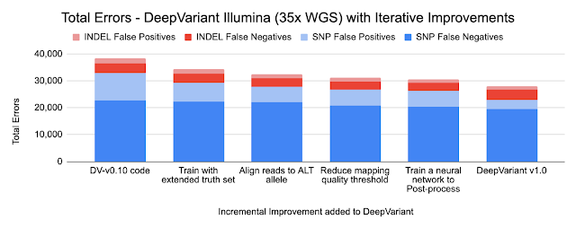
Because DeepVariant is a deep learning method, we can quickly re-train it for these new instrument types, ensuring highly accurate sequence identification. Accuracy is important because a missed variant call could mean missing the causal variant for a disorder, while a false positive variant call could lead to identifying an incorrect one. Earlier state-of-the-art methods could reach ~99.1% accuracy (~73,000 errors) on a 35-fold coverage Illumina whole genome, whereas an early version of DeepVariant (v0.10) had ~99.4% accuracy (46,000 errors), corresponding to a 38% error reduction. DeepVariant v1.0 reduces Illumina errors by another ~22% and PacBio errors by another ~52% relative to the last DeepVariant release (v0.10).

DeepVariant Overview
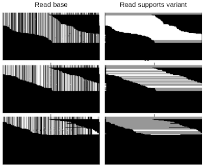
DeepVariant is a convolutional neural network (CNN) that treats the task of identifying genetic variants as an image classification problem. DeepVariant constructs tensors, essentially multi-channel images, where each channel represents an aspect of the sequence, such as the bases in the sequence (called read base), the quality of alignment between different reads (mapping quality), whether a given read supports an alternate allele (read supports variant), etc. It then analyzes these data and outputs three genotype likelihoods, corresponding to how many copies (0, 1, or 2) of a given alternate allele are present.

Example of DeepVariant data. Each row of pixels in each panel corresponds to a single read, i.e., a short genetic sequence. The top, middle, and bottom rows of panels present examples with a different number of variant alleles. Only two of the six data channels are shown: Read base — the pixel value is mapped to each of the four bases, A, C, G, or T; Read supports variant — white means that the read is consistent with a given allele and grey means it is not. Top: Classified by DeepVariant as a "2", which means that both chromosomes match the variant allele. Middle: Classified as a “1”, meaning that one chromosome matches the variant allele. Bottom: Classified as a “0”, implying that the variant allele is missing from both chromosomes.

Technical Improvements in DeepVariant v1.0
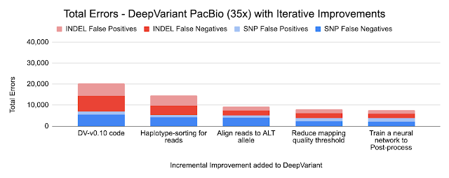
Because DeepVariant uses the same codebase for each data type, improvements apply to each of Illumina, PacBio, and Oxford Nanopore. Below, we show the numbers for Illumina and PacBio for two types of small variants: SNPs (single nucleotide polymorphisms, which change a single base without changing sequence length) and INDELs (insertions and deletions).

  • Training on an extended truth set

    The Genome in a Bottle consortium from the National Institute of Standards and Technology (NIST) creates gold-standard samples with known variants covering the regions of the genome. These are used as labels to train DeepVariant. Using long-read technologies the Genome in a Bottle expanded the set of confident variants, increasing the regions described by the standard set from 85% of the genome to 92% of it. These more difficult regions were already used in training the PacBio models, and including them in the Illumina models reduced errors by 11%. By relaxing the filter for reads of lower mapping quality, we further reduced errors by 4% for Illumina and 13% for PacBio.

  • Haplotype sorting of long reads

    We inherit one copy of DNA from our mother and another from our father. PacBio and Oxford Nanopore sequences are long enough to separate sequences by parental origin, which is called a haplotype. By providing this information to the neural network, DeepVariant improves its identification of random sequence errors and can better determine whether a variant has a copy from one or both parents.

  • Re-aligning reads to the alternate (ALT) allele

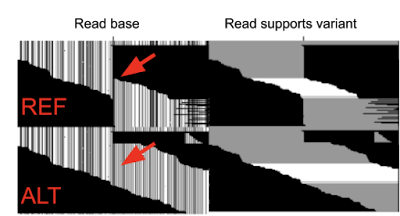
    DeepVariant uses input sequence fragments that have been aligned to a reference genome. The optimal alignment for variants that include insertions or deletions could be different if the aligner knew they were present. To capture this information, we implemented an additional alignment step relative to the candidate variant. The figure below shows an additional second row where the reads are aligned to the candidate variant, which is a large insertion. You can see sequences that abruptly stop in the first row can now be fully aligned, providing additional information.

    Example of DeepVariant data with realignment to ALT allele. DeepVariant is presented the information in both rows of data for the same example. Only two of the six data channels are shown: Read base (channel #1) and Read supports variant (channel #5). Top: Shows the reads aligned to the reference (in DeepVariant v0.10 and earlier this is all DeepVariant sees). Bottom: Shows the reads aligned to the candidate variant, in this case a long insertion of sequence). The red arrow indicates where the inserted sequence begins.
  • Use a small network to post-process outputs

    Variants can have multiple alleles, with a different base inherited from each parent. DeepVariant’s classifier only generates a probability for one potential variant at a time. In previous versions, simple hand-written rules converted the probabilities into a composite call, but these rules failed in some edge cases. In addition, it also separated the way a final call was made from the backpropagation to train the network. By adding a small, fully-connected neural network to the post-processing step, we are able to better handle these tricky multi-allelic cases.

  • Adding data to train the release model

    The timeframe for the competition was compressed, so we trained only with data similar to the challenge data (PCR-Free NovaSeq) to speed model training. In our production releases, we seek high accuracy for multiple instruments as well as PCR+ preparations. Training with data from these diverse classes helps the model generalize, so our DeepVariant v1.0 release model outperforms the one submitted.

The charts below show the error reduction achieved by each improvement.

Training a Hybrid model
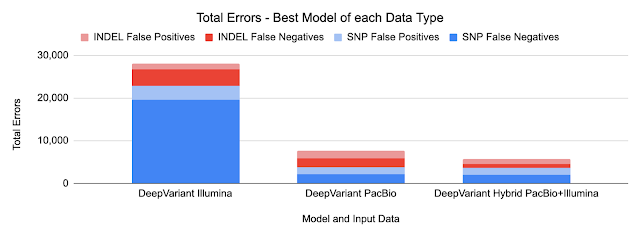
DeepVariant v1.0 also includes a hybrid model for PacBio and Illumina reads. In this case, the model leverages the strengths of both input types, without needing new logic.

Example of DeepVariant merging data from both PacBio and Illumina. Only two of the six data channels are shown: Read base (channel #1) and Read supports variant (channel #5). The longer PacBio reads (at the upper part of the image) span the region being called entirely, while the shorter Illumin reads span only a portion of the region.

We observed no change in SNP errors, suggesting that PacBio reads are strictly superior for SNP calling. We observed a further 49% reduction in Indel errors relative to the PacBio model, suggesting that the Indel error modes of Illumina and PacBio HiFi can be used in a complementary manner.

PEPPER-Deepvariant: A Pipeline for Oxford Nanopore Data Using DeepVariant
Until the PrecisionFDA competition, a DeepVariant model was not available for Oxford Nanopore data, because the higher base error rate created too many candidates for DeepVariant to classify. We partnered with the UC Santa Cruz Genomics Institute, which has extensive expertise with Nanopore data. They had previously trained a deep learning method called PEPPER, which could narrow down the candidates to a more tractable number. The larger neural network of DeepVariant can then accurately characterize the remaining candidates with a reasonable runtime.

The combined PEPPER-DeepVariant pipeline with the Oxford Nanopore model is open-source and available on GitHub. This pipeline was able to achieve a superior SNP calling accuracy to DeepVariant Illumina on the PrecisionFDA challenge, which is the first time anyone has shown Nanopore outperforming Illumina in this way.

Conclusion
DeepVariant v1.0 isn’t the end of development. We look forward to working with the genomics community to further maximize the value of genomic data to patients and researchers.

Source: Google AI Blog


KeyPose: Estimating the 3D Pose of Transparent Objects from Stereo

Estimating the position and orientation of 3D objects is one of the core problems in computer vision applications that involve object-level perception, such as augmented reality and robotic manipulation. In these applications, it is important to know the 3D position of objects in the world, either to directly affect them, or to place simulated objects correctly around them. While there has been much research on this topic using machine learning (ML) techniques, especially Deep Nets, most have relied on the use of depth sensing devices, such as the Kinect, which give direct measurements of the distance to an object. For objects that are shiny or transparent, direct depth sensing does not work well. For example, the figure below includes a number of objects (left), two of which are transparent stars. A depth device does not find good depth values for the stars, and gives a very poor reconstruction of the actual 3D points (right).
Left: RGB image of transparent objects.  Right: A four-panel image showing the reconstructed depth for the scene on the left.The top row includes depth images and the bottom row presents the 3D point cloud. The left panels were reconstructed using a depth camera and the right panels are output from the ClearGrasp model.  Note that although ClearGrasp inpaints the depth of the stars, it mistakes the actual depth of the rightmost one.

One solution to this problem, such as that proposed by ClearGrasp, is to use a deep neural network to inpaint the corrupted depth map of the transparent objects. Given a single RGB-D image of transparent objects, ClearGrasp uses deep convolutional networks to infer surface normals, masks of transparent surfaces, and occlusion boundaries, which it uses to refine the initial depth estimates for all transparent surfaces in the scene (far right in the figure above). This approach is very promising, and allows scenes with transparent objects to be processed by pose-estimation methods that rely on depth.  But inpainting can be tricky, especially when trained completely with synthetic images, and can still result in errors in depth.

In “KeyPose: Multi-View 3D Labeling and Keypoint Estimation for Transparent Objects”, presented at CVPR 2020 in collaboration with the Stanford AI Lab, we describe an ML system that estimates the depth of transparent objects by directly predicting 3D keypoints. To train the system we gather a large real-world dataset of images of transparent objects in a semi-automated way, and efficiently label their pose using 3D keypoints selected by hand. We then train deep models (called KeyPose) to estimate the 3D keypoints end-to-end from monocular or stereo images, without explicitly computing depth. The models work on objects both seen and unseen during training, for both individual objects and categories of objects. While KeyPose can work with monocular images, the extra information available from stereo images allows it to improve its results by a factor of two over monocular image input, with typical errors from 5 mm to 10 mm, depending on the objects. It substantially improves over state-of-the-art in pose estimation for these objects, even when competing methods are provided with ground truth depth. We are releasing the dataset of keypoint-labeled transparent objects for use by the research community.

Real-World Transparent Object Dataset with 3D Keypoint Labels
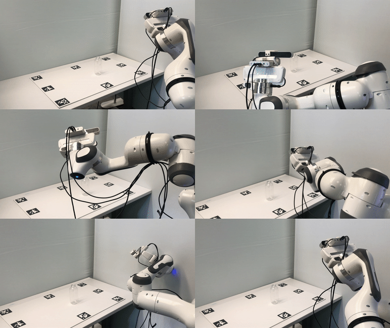
To facilitate gathering large quantities of real-world images, we set up a robotic data-gathering system in which a robot arm moves through a trajectory while taking video with two devices, a stereo camera and the Kinect Azure depth camera.

Automated image sequence capture using a robot arm with a stereo camera and an Azure Kinect device.

The AprilTags on the target enable accurate tracing of the pose of the cameras. By hand-labelling only a few images in each video with 2D keypoints, we can extract 3D keypoints for all frames of the video using multi-view geometry, thus increasing the labelling efficiency by a factor of 100.

We captured imagery for 15 different transparent objects in five categories, using 10 different background textures and four different poses for each object, yielding a total of 600 video sequences comprising 48k stereo and depth images. We also captured the same images with an opaque version of the object, to provide accurate ground truth depth images. All the images are labelled with 3D keypoints. We are releasing this dataset of real-world images publicly, complementing the synthetic ClearGrasp dataset with which it shares similar objects.

KeyPose Algorithm Using Early Fusion Stereo
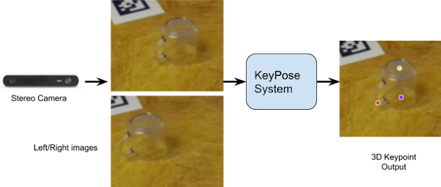
The idea of using stereo images directly for keypoint estimation was developed independently for this project; it has also appeared recently in the context of hand-tracking. The diagram below shows the basic idea: the two images from a stereo camera are cropped around the object and fed to the KeyPose network, which predicts a sparse set of 3D keypoints that represent the 3D pose of the object. The network is trained using supervision from the labelled 3D keypoints.

One of the key aspects of stereo KeyPose is the use of early fusion to intermix the stereo images, and allow the network to implicitly compute disparity, in contrast to late fusion, in which keypoints are predicted for each image separately, and then combined. As shown in the diagram below, the output of KeyPose is a 2D keypoint heatmap in the image plane along with a disparity (i.e., inverse depth) heatmap for each keypoint. The combination of these two heatmaps yields the 3D coordinate of the keypoint, for each keypoint.

Keypose system diagram. Stereo images are passed to a CNN model to produce a probability heatmap for each keypoint.  This heatmap yields 2D image coordinates U,V for the keypoint.  The CNN model also produces a disparity (inverse depth) heatmap for each keypoint, which when combined with the U,V coordinates, gives a 3D position (X,Y,Z).

When compared to late fusion or to monocular input, early fusion stereo typically is twice as accurate.

Results
The images below show qualitative results of KeyPose on individual objects. On the left is one of the original stereo images; in the middle are the predicted 3D keypoints projected onto the image. On the right, we visualize points from a 3D model of the bottle, placed at the pose determined by the predicted 3D keypoints. The network is efficient and accurate, predicting keypoints with an MAE of 5.2 mm for the bottle and 10.1 mm for the mug using just 5 ms on a standard GPU.

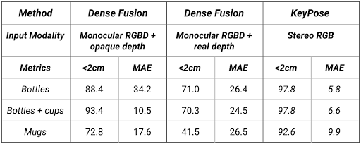
The following table shows results for KeyPose on category-level estimation. The test set used a background texture not seen by the training set. Note that the MAE varies from 5.8 mm to 9.9 mm, showing the accuracy of the method.

Quantitative comparison of KeyPose with the state-of-the-art DenseFusion system, on category-level data. We provide DenseFusion with two versions of depth, one from the transparent objects, and one from opaque objects. <2cm is the percent of estimates with errors less than 2 cm. MAE is the mean absolute error of the keypoints, in mm.

For a complete accounting of quantitative results, as well as, ablation studies, please see the paper and supplementary materials and the KeyPose website.

Conclusion
This work shows that it is possible to accurately estimate the 3D pose of transparent objects from RGB images without reliance on depth images. It validates the use of stereo images as input to an early fusion deep net, where the network is trained to extract sparse 3D keypoints directly from the stereo pair. We hope the availability of an extensive, labelled dataset of transparent objects will help to advance the field. Finally, while we used semi-automatic methods to efficiently label the dataset, we hope to employ self-supervision methods in future work to do away with manual labelling.

Acknowledgements
I want to thank my co-authors, Xingyu Liu of Stanford University, and Rico Jonschkowski and Anelia Angelova; as well the many who helped us through discussions during the project and paper writing, including Andy Zheng, Shuran Song, Vincent Vanhoucke, Pete Florence, and Jonathan Tompson.

Source: Google AI Blog


Understanding View Selection for Contrastive Learning

Most people take for granted the ability to view an object from several different angles, but still recognize that it's the same object— a dog viewed from the front is still a dog when viewed from the side. While people do this naturally, computer scientists need to explicitly enable machines to learn representations that are view-invariant, with the goal of seeking robust data representations that retain information that is useful to downstream tasks.

Of course, in order to learn these representations, manually annotated training data can be used. However, as in many cases such annotations aren’t available, which gives rise to a series of self- and crossmodal supervised approaches that do not require manually annotated training data. Currently, a popular paradigm for training with such data is contrastive multiview learning, where two views of the same scene (for example, different image channels, augmentations of the same image, and video and text pairs) will tend to converge in representation space while two views of different scenes diverge. Despite their success, one important question remains: “If one doesn’t have annotated labels readily available, how does one select the views to which the representations should be invariant?” In other words, how does one identify an object using information that resides in the pixels of the image itself, while still remaining accurate when that image is viewed from disparate viewpoints?

In “What makes for good views for contrastive learning”, we use theoretical and empirical analysis to better understand the importance of view selection, and argue that one should reduce the mutual information between views while keeping task-relevant information intact. To verify this hypothesis, we devise unsupervised and semi-supervised frameworks that learn effective views by aiming to reduce their mutual information. We also consider data augmentation as a way to reduce mutual information, and show that increasing data augmentation indeed leads to decreasing mutual information while improving downstream classification accuracy. To encourage further research in this space, we have open-sourced the code and pre-trained models.
The InfoMin Hypothesis
The goal of contrastive multiview learning is to learn a parametric encoder, whose output representations can be used to discriminate between pairs of views with the same identities, and pairs with different identities. The amount and type of information shared between the views determines how well the resulting model performs on downstream tasks. We hypothesize that the views that yield the best results should discard as much information in the input as possible except for the task relevant information (e.g., object labels), which we call the InfoMin principle.

Consider the example below in which two patches of the same image represent the different “views”. The training objective is to identify that the two views belong to the same image. It is undesirable to have views that share too much information, for example, where low-level color and texture cues can be exploited as “shortcuts” (left), or to have views that share too little information to identify that they belong to the same image (right). Rather, views at the “sweet spot” share the information related to downstream tasks, such as patches corresponding to different parts of the panda for an object classification task (center).

An illustration of three regimes of information captured during contrastive multiview learning. Views should not share too much information (left) or too little information (right), but should find an optimal mix (the “sweet spot”, middle) that maximizes the downstream performance.

A Unified View on Contrastive Learning
We design several sets of experiments to verify the InfoMin hypothesis, motivated by the fact that there are simple ways to control the mutual information shared between views without any supervision. For example, we can sample different patches from the same images, and reduce their mutual information simply by increasing the distance between the patches. Here, we estimate the mutual information using InfoNCE (INCE), which is a quantitative measure of the mutual information lower bound.. Indeed, we observe a reverse U-shape curve: as mutual information is reduced, the downstream task accuracy first increases and then begins to decrease.

Downstream classification accuracy on STL-10 (left) and CIFAR-10 (right) by applying linear classifiers on representations learned with contrastive learning. Same as the previous illustration, the views are sampled as different patches from the same images. Increasing the Euclidean distance between patches leads to decreasing mutual information. A reverse U-shape curve between classification accuracy and INCE (patch distance) is observed.

Furthermore, we demonstrate that several state-of-the-art contrastive learning methods (InstDis, MoCo, CMC, PIRL, SimCLR and CPC) can be unified through the perspective of view selection: despite the differences in architecture, objective and engineering details, all recent contrastive learning methods create two views that implicitly follow the InfoMin hypothesis, where the information shared between views are controlled by the strength of data augmentation. Motivated by this, we propose a new set of data augmentations, which outperforms the prior state of the art, SimCLR, by nearly 4% on the ImageNet linear readout benchmark. We also found that transferring our unsupervised pre-trained models to object detection and instance segmentation consistently outperforms ImageNet pre-training.

Learning to Generate Views
In our work, we design unsupervised and semi-supervised methods that synthesize novel views following the InfoMin hypothesis. We learn flow-based models that transfer natural color spaces into novel color spaces, from which we split the channels to get views. For the unsupervised setup, the view generators are optimized to minimize the InfoNCE bound between views. As shown in the results below, we observe a similar reverse U-shape trend while minimizing the InfoNCE bound.

View generators learned by unsupervised (left) and semi-supervised (right) objectives.

To reach the sweet spot without overly minimizing mutual information, we can use the semi-supervised setup and guide the view generator to retain label information. As expected, all learned views are now centered around the sweet spot, no matter what the input color space is.

Code and Pretrained Models
To accelerate research in self-supervised contastive learning, we are excited to share the code and pretrained models of InfoMin with the academic community. They can be found here.

Acknowledgements
The core team includes Yonglong Tian, Chen Sun, Ben Poole, Dilip Krishnan, Cordelia Schmid and Phillip Isola. We would like to thank Kevin Murphy for insightful discussion; Lucas Beyer for feedback on the manuscript; and the Google Cloud team for computation support.
Source: Google AI Blog


On-device, Real-time Body Pose Tracking with MediaPipe BlazePose

Pose estimation from video plays a critical role enabling the overlay of digital content and information on top of the physical world in augmented reality, sign language recognition, full-body gesture control, and even quantifying physical exercises, where it can form the basis for yoga, dance, and fitness applications. Pose estimation for fitness applications is particularly challenging due to the wide variety of possible poses (e.g., hundreds of yoga asanas), numerous degrees of freedom, occlusions (e.g. the body or other objects occlude limbs as seen from the camera), and a variety of appearances or outfits.

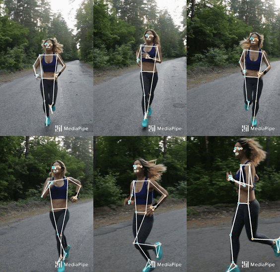
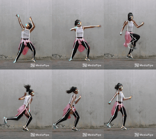
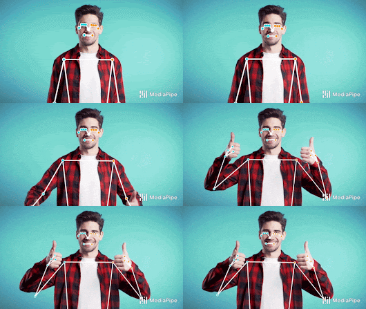
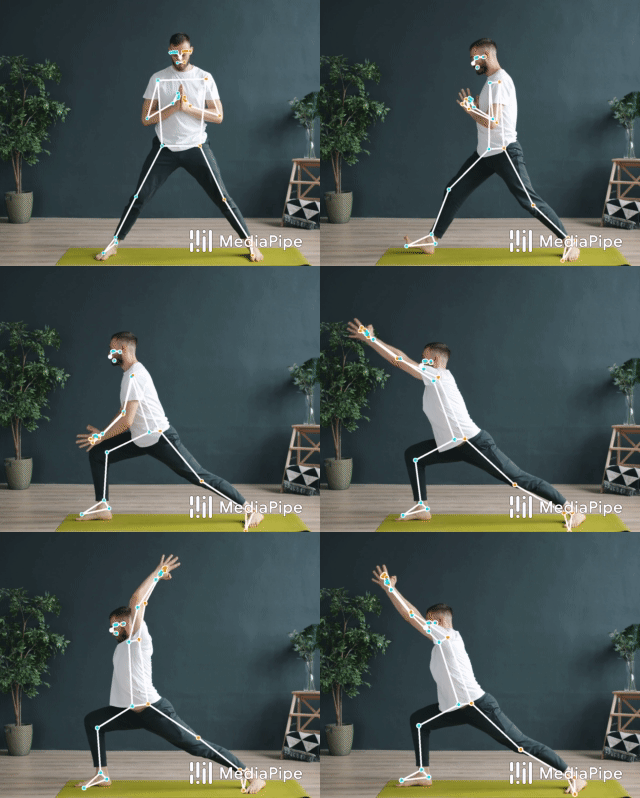
BlazePose results on fitness and dance use-cases.

Today we are announcing the release of a new approach to human body pose perception, BlazePose, which we presented at the CV4ARVR workshop at CVPR 2020. Our approach provides human pose tracking by employing machine learning (ML) to infer 33, 2D landmarks of a body from a single frame. In contrast to current pose models based on the standard COCO topology, BlazePose accurately localizes more keypoints, making it uniquely suited for fitness applications. In addition, current state-of-the-art approaches rely primarily on powerful desktop environments for inference, whereas our method achieves real-time performance on mobile phones with CPU inference. If one leverages GPU inference, BlazePose achieves super-real-time performance, enabling it to run subsequent ML models, like face or hand tracking.

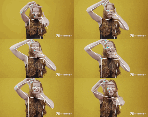
Upper-body BlazePose model in MediaPipe

Topology
The current standard for human body pose is the COCO topology, which consists of 17 landmarks across the torso, arms, legs, and face. However, the COCO keypoints only localize to the ankle and wrist points, lacking scale and orientation information for hands and feet, which is vital for practical applications like fitness and dance. The inclusion of more keypoints is crucial for the subsequent application of domain-specific pose estimation models, like those for hands, face, or feet.

With BlazePose, we present a new topology of 33 human body keypoints, which is a superset of COCO, BlazeFace and BlazePalm topologies. This allows us to determine body semantics from pose prediction alone that is consistent with face and hand models.

BlazePose 33 keypoint topology as COCO (colored with green) superset

Overview: An ML Pipeline for Pose Tracking
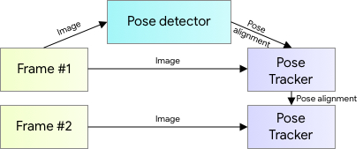
For pose estimation, we utilize our proven two-step detector-tracker ML pipeline. Using a detector, this pipeline first locates the pose region-of-interest (ROI) within the frame. The tracker subsequently predicts all 33 pose keypoints from this ROI. Note that for video use cases, the detector is run only on the first frame. For subsequent frames we derive the ROI from the previous frame’s pose keypoints as discussed below.

Human pose estimation pipeline overview.

Pose Detection by extending BlazeFace
For real-time performance of the full ML pipeline consisting of pose detection and tracking models, each component must be very fast, using only a few milliseconds per frame. To accomplish this, we observe that the strongest signal to the neural network about the position of the torso is the person's face (due to its high-contrast features and comparably small variations in appearance). Therefore, we achieve a fast and lightweight pose detector by making the strong (yet for many mobile and web applications valid) assumption that the head should be visible for our single-person use case.

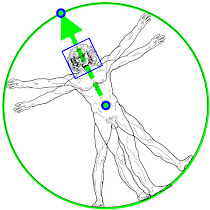
Consequently, we trained a face detector, inspired by our sub-millisecond BlazeFace model, as a proxy for a pose detector. Note, this model only detects the location of a person within the frame and can not be used to identify individuals. In contrast to the Face Mesh and MediaPipe Hand tracking pipelines, where we derive the ROI from predicted keypoints, for the human pose tracking we explicitly predict two additional virtual keypoints that firmly describe the human body center, rotation and scale as a circle. Inspired by Leonardo’s Vitruvian man, we predict the midpoint of a person's hips, the radius of a circle circumscribing the whole person, and the incline angle of the line connecting the shoulder and hip midpoints. This results in consistent tracking even for very complicated cases, like specific yoga asanas. The figure below illustrates the approach.

Vitruvian man aligned via two virtual keypoints predicted by our BlazePose detector in addition to the face bounding box

Tracking Model
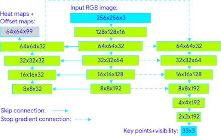
The pose estimation component of the pipeline predicts the location of all 33 person keypoints with three degrees of freedom each (x, y location and visibility) plus the two virtual alignment keypoints described above. Unlike current approaches that employ compute-intensive heatmap prediction, our model uses a regression approach that is supervised by a combined heat map/offset prediction of all keypoints, as shown below.

Tracking network architecture: regression with heatmap supervision

Specifically, during training we first employ a heatmap and offset loss to train the center and left tower of the network. We then remove the heatmap output and train the regression encoder (right tower), thus, effectively using the heatmap to supervise a lightweight embedding.

The table below shows an ablation study of the model quality resulting from different training strategies. As an evaluation metric, we use the Percent of Correct Points with 20% tolerance ([email protected]) (where we assume the point to be detected correctly if the 2D Euclidean error is smaller than 20% of the corresponding person’s torso size). To obtain a human baseline, we asked annotators to annotate several samples redundantly and obtained an average [email protected] of 97.2. The training and validation have been done on a geo-diverse dataset of various poses, sampled uniformly.

To cover a wide range of customer hardware, we present two pose tracking models: lite and full, which are differentiated in the balance of speed versus quality. For performance evaluation on CPU, we use XNNPACK; for mobile GPUs, we use the TFLite GPU backend.

Applications
Based on human pose, we can build a variety of applications, like fitness or yoga trackers. As an example, we present squats and push up counters, which can automatically count user statistics, or verify the quality of performed exercises. Such use cases can be implemented either using an additional classifier network or even with a simple joint pairwise distance lookup algorithm, which matches the closest pose in normalized pose space.

The number of performed exercises counter based on detected body pose. Left: Squats; Right: Push-Ups

Conclusion
BlazePose will be available to the broader mobile developer community via the Pose detection API in the upcoming release of ML Kit, and we are also releasing a version targeting upper body use cases in MediaPipe running in Android, iOS and Python. Apart from the mobile domain, we preview our web-based in-browser version as well. We hope that providing this human pose perception functionality to the broader research and development community will result in an emergence of creative use cases, stimulating new applications, and new research avenues.

We plan to extend this technology with more robust and stable tracking to an even larger variety of human poses and activities. In the accompanying Model Card, we detail the intended uses, limitations and model fairness to ensure that use of these models aligns with Google’s AI Principles. We believe that publishing this technology can provide an impulse to new creative ideas and applications by the members of the research and developer community at large. We are excited to see what you can build with it!

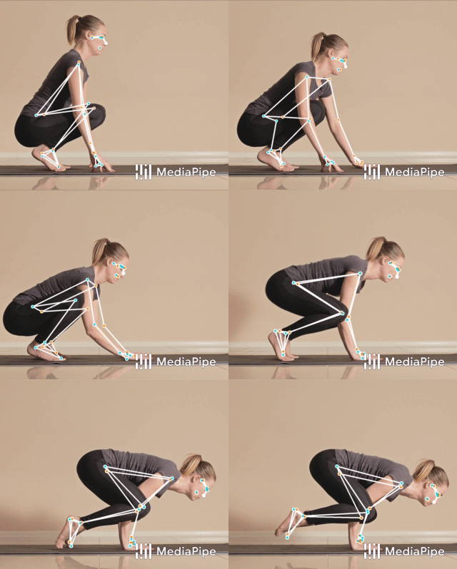
BlazePose results on yoga use-cases

Acknowledgments
Special thanks to all our team members who worked on the tech with us: Fan Zhang, Artsiom Ablavatski, Yury Kartynnik, Tyler Zhu, Karthik Raveendran, Andrei Vakunov, Andrei Tkachenka, Marat Dukhan, Tyler Mullen, Gregory Karpiak, Suril Shah, Buck Bourdon, Jiuqiang Tang, Ming Guang Yong, Chuo-Ling Chang, Esha Uboweja, Siarhei Kazakou, Andrei Kulik, Matsvei Zhdanovich, and Matthias Grundmann.

Source: Google AI Blog


REALM: Integrating Retrieval into Language Representation Models

Recent advances in natural language processing have largely built upon the power of unsupervised pre-training, which trains general purpose language representation models using a large amount of text, without human annotations or labels. These pre-trained models, such as BERT and RoBERTa, have been shown to memorize a surprising amount of world knowledge, such as “the birthplace of Francesco Bartolomeo Conti”, “the developer of JDK” and “the owner of Border TV”. While the ability to encode knowledge is especially important for certain natural language processing tasks such as question answering, information retrieval and text generation, these models memorize knowledge implicitly — i.e., world knowledge is captured in an abstract way in the model weights — making it difficult to determine what knowledge has been stored and where it is kept in the model. Furthermore, the storage space, and hence the accuracy of the model, is limited by the size of the network. To capture more world knowledge, the standard practice is to train ever-larger networks, which can be prohibitively slow or expensive.

Instead, what if there was a method for pre-training that could access knowledge explicitly, e.g., by referencing an additional large external text corpus, in order to achieve accurate results without increasing the model size or complexity?  For example, a sentence found in an external document collection, "Francesco Bartolomeo Conti was born in Florence," could be referenced by the model to determine the birthplace of the musician, rather than relying on the model's opaque ability to access the knowledge stored in its own parameters. The ability to retrieve text containing explicit knowledge such as this would improve the efficiency of pre-training while enabling the model to perform well on knowledge-intensive tasks without using billions of parameters.

In “REALM: Retrieval-Augmented Language Model Pre-Training”, accepted at the 2020 International Conference on Machine Learning, we share a novel paradigm for language model pre-training, which augments a language representation model with a knowledge retriever, allowing REALM models to retrieve textual world knowledge explicitly from raw text documents, instead of memorizing all the knowledge in the model parameters. We have also open sourced the REALM codebase to demonstrate how one can train the retriever and the language representation jointly.

Background: Pre-training Language Representation Models
To understand how standard language representation models memorize world knowledge, one should first review how these models are pre-trained. Since the invention of BERT, the fill-in-the-blank task, called masked language modeling, has been widely used for pre-training language representation models. Given any text with certain words masked out, the task is to fill back the missing words. An example of this task looks like:

I am so thirsty. I need to __ water.

During pre-training, a model will go over a large number of examples and adjust the parameters in order to predict the missing words (answer: drink, in the above example). Interestingly, the fill-in-the-blank task makes the model memorize certain facts about the world. For example, the knowledge of Einstein's birthplace is required to fill the missing word in the following example:

Einstein was a __-born scientist. (answer: German)

However, because the world knowledge captured by the model is stored in the model weights, it is abstract, making it difficult to understand what information is stored.

Our Proposal: Retrieval-Augmented Language Representation Model Pre-training
In contrast to standard language representation models, REALM augments the language representation model with a knowledge retriever that first retrieves another piece of text from an external document collection as the supporting knowledge — in our experiments, we use the Wikipedia text corpus — and then feeds this supporting text as well as the original text into a language representation model.

The key intuition of REALM is that a retrieval system should improve the model's ability to fill in missing words. Therefore, a retrieval that provides more context for filling the missing words should be rewarded. If the retrieved information does not help the model make its predictions, it should be discouraged, making room for better retrievals.

How does one train a knowledge retriever, given that only unlabeled text is available during pre-training? It turns out that one can use the task of filling words to train the knowledge retriever indirectly, without any human annotations. Assume the input of the query is:

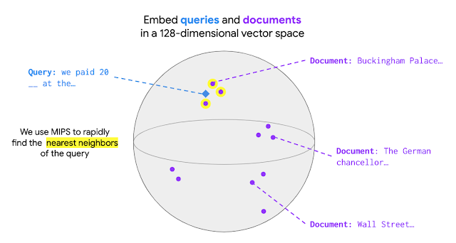
We paid twenty __ at the Buckingham Palace gift shop.

Filling the missing word (answer:pounds) in this sentence without retrieval can be tricky, as the model would need to have implicitly stored knowledge of the country in which the Buckingham Palace is located and the associated currency, as well as make the connection between the two. It would be easier for the model to fill in the missing word if it was presented with a passage that explicitly connects some of the necessary knowledge, retrieved from an external corpus.

In this example, the retriever would be rewarded for retrieving the following sentence.

Buckingham Palace is the London residence of the British monarchy.

Since the retrieval step needs to add more context, there may be multiple retrieval targets that could be helpful in filling the missing word, for example, “The official currency of the United Kingdom is the Pound.” The whole process is demonstrated in the next figure:

Computational Challenges for REALM
Scaling REALM pre-training such that models can retrieve knowledge from millions of documents is challenging. In REALM, the selection of the best document is formulated as maximum inner product search (MIPS). To perform retrieval, MIPS models need to first encode all of the documents in the collection, such that each document has a corresponding document vector. When an input arrives, it is encoded as a query vector. In MIPS, given a query, the document in the collection that has the maximum inner product value between its document vector and the query vector is retrieved, as shown in the following figure:

In REALM, we use the ScaNN package to conduct MIPS efficiently, which makes finding the maximum inner product value relatively cheap, given that the document vectors are pre-computed. However, if the model parameters were updated during training, it is typically necessary to re-encode the document vectors for the entire collection of documents. To address the computational challenges, we structure the retriever so that the computation performed for each document can be cached and asynchronously updated. We also found that updating document vectors every 500 training steps, instead of every step, is able to achieve good performance and make training tractable.

Applying REALM to Open-domain Question Answering
We evaluate the effectiveness of REALM by applying it to open-domain question answering (Open-QA), one of the most knowledge-intensive tasks in natural language processing. The goal of the task is to answer questions, such as “What is the angle of the equilateral triangle?”

In standard question answering tasks (e.g., SQuAD or Natural Questions), the supporting document is provided as part of input, so a model only needs to look up the answer in the given document. In Open-QA, there are no given documents, so that Open-QA models need to look up the knowledge by themselves — this makes Open-QA an excellent task to examine the effectiveness of REALM.

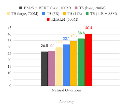
The following figure shows the results on the OpenQA version of Natural Question. We mainly compared our results with T5, another approach that trains models without annotated supporting documents. From the figure, one can clearly see that REALM pre-training generates very powerful Open-QA models, and even outperforms the much larger T5 (11B) model by almost 4 points, using only a fraction of the parameters (300M).

Conclusion
The release of REALM has helped drive interest in developing end-to-end retrieval-augmented models, including a recent retrieval-augmented generative model. We look forward to the possibility of extending this line of work in several ways, including 1) applying REALM-like methods to new applications that require knowledge-intensive reasoning and interpretable provenance (beyond Open-QA), and 2) exploring the benefits of retrieving other forms of knowledge, such as images, knowledge graph structures, or even text in other languages. We are also excited to see what the research community does with the open source REALM codebase!

Acknowledgements
This work has been a collaborative effort involving Kelvin Guu, Kenton Lee, Zora Tung, Panupong Pasupat and Ming-Wei Chang.

Source: Google AI Blog


On-device Supermarket Product Recognition


One of the greatest challenges faced by users who are visually impaired is identifying packaged foods, both in a grocery store and also in their kitchen cupboard at home. This is because many foods share the same packaging, such as boxes, tins, bottles and jars, and only differ in the text and imagery printed on the label. However, the ubiquity of smart mobile devices provides an opportunity to address such challenges using machine learning (ML).

In recent years, there have been significant improvements in the accuracy of on-device neural networks for various perception tasks. When coupled with the increased computing power in modern smartphones, it is now possible for many vision tasks to yield high performance while running entirely on a mobile device. The development of on-device models such as MnasNet and MobileNets (based on resource-aware architecture search) in combination with on-device indexing allows one to run a full computer vision system, such as labeled product recognition, entirely on-device, in real time.

Leveraging developments such as these, we recently released Lookout, an Android app that uses computer vision to make the physical world more accessible for users who are visually impaired. When the user aims their smartphone camera at the product, Lookout identifies it and speaks aloud the brand name and product size. To accomplish this, Lookout includes a supermarket product detection and recognition model with an on-device product index, along with MediaPipe object tracking and an optical character recognition model. The resulting architecture is efficient enough to run in real-time entirely on-device.

Why On-Device?
A completely on-device system has the benefit of being low latency and with no reliance on network connectivity. However, this means that for a product recognition system to be truly useful to the users, it must have a on-device database with good product coverage. These requirements drive the design of the datasets used by Lookout, which consist of two million popular products chosen dynamically according to the user’s geographic location.

Traditional Solutions
Product recognition using computer vision has traditionally been solved using local image features extracted by, for example, the SIFT algorithm. These non ML-based approaches provide fairly reliable matching but are storage intensive per index image (typically ranging from 10KB to 40KB per image) and are less robust to poor lighting and blur in images. Additionally, the local nature of these descriptors means that it typically does not capture more global aspects of the product’s appearance.

An alternative approach that has a number of advantages would be to use ML and run an optical character recognition (OCR) system over the query image and database images to extract the text present on the product packaging. The text on the query image can be matched to the database using N-Grams to be robust to OCR errors such as spelling mistakes, misrecognitions, failed recognition of words on product packaging. N-Grams can also allow for partial match between query document and index document using measures such as Jaccard similarity coefficient, as opposed to requiring an exact match. However, with OCR, the index document size can grow very large since one would need to store N-Grams for product packaging text along with other signals like TF-IDF. Furthermore, the reliability of the matches is a concern with the OCR+N-Gram approach since it can easily over trigger in situations where there are a lot of common words present on the packaging of two different products.

In contrast to both the SIFT and OCR+N-Gram methods, our neural network-based approach, which generates a global descriptor (i.e., an embedding) for each image, requires only 64 bytes, significantly reducing the storage requirements from the 10-40KB per image needed for each SIFT feature index entry, or the few KBs per image for the less reliable OCR+N-gram approach. With fewer bytes consumed for each index image, more products can be included as a part of the index, yielding more complete product coverage and a better overall user experience.

Design
The Lookout system consists of a frame cache, frame selector, detector, object tracker, embedder, index searcher, OCR, scorer and result presenter.
Product recognition pipeline internal architecture.
  • Frame cache
    The frame cache manages the lifecycle of the input camera frames in the pipeline. It efficiently delivers the data, including YUV/RGB/gray images, as requested by the other model components and manages the data life cycle to avoid duplicated conversions for the same camera frame requested by multiple components.
  • Frame selector
    When a user points the camera viewfinder towards a product, a lightweight IMU-based frame selector is run as a prefiltering stage. It selects the frames that best match a certain quality criterion (e.g., balanced image quality and latency) from the continuously incoming image stream, based on the jitter as measured by the angular rotation rate (deg/sec). This approach minimizes energy consumption by selectively processing only the high quality image frames and skipping the blurry frames.
  • Detector
    Each selected frame is then passed to a product detector model, which proposes regions of interest(a.k.a. Detection bounding boxes) in the frames. The detector model architecture is a single-shot detector with an MnasNet backbone that strikes a balance between high quality and low latency.
  • Object tracker
    MediaPipe Box tracking is used to track the detected box in real-time, and plays an important role in filling the gap between the detection of different objects and reducing the detection frequency, thus reducing energy consumption. The object tracker also maintains an object map in which each object is assigned a unique object ID during runtime, which are later used by the result presenter to differentiate between objects and to avoid repeating the announcement of a single object. For each detection result, the tracker either registers a new object in the map or updates an existing object with the detection bounding box, using the Intersection over Union (IoU) between existing object bounding boxes with the detection result.
  • Embedder
    The regions of interest (ROIs) from the detector are sent to the embedder model, which then computes a 64-dimension embedding. The embedder model is initially trained from a large classification model (i.e., the teacher model, based on NASNet), which spans tens of thousands of classes. An embedding layer is added in the model to project the input image into an ‘embedding space’, i.e., a vector space where two points being close means that the images they represent are visually similar (e.g., two images show the same product). Analyzing only the embeddings ensures that the model is flexible and does not need to be retrained every time it is to be expanded to new products. However, because the teacher model is too large to be used directly on-device, the embeddings it generates are used to train a smaller, mobile-friendly student model that learns to map the input images to the same points in the embedding space as the teacher network. Finally, we apply principal component analysis (PCA) to reduce the dimensionality of the embedding vectors from 256 to 64, streamlining the embeddings for storing on-device.
  • Index searcher
    The index searcher performs KNN search over a pre-built, compatible ScaNN index using a query embedding. As a result, it returns the top-ranked index documents containing their metadata, such as product names, packaging size, etc. To reduce the index lookup latency, all embeddings are k-means clustered into clusters. At query time, the relevant clusters of data are loaded in memory for the actual distance computation. To reduce the index size without sacrificing quality, we use product quantization at indexing time.
  • OCR
    OCR is executed on the ROI for each camera frame in order to extract additional information, such as packet size, product flavor variant, etc. Whereas traditional solutions used the OCR result for index searching, here we only use it for scoring. A proper scoring algorithm informed by the OCR text assists the scorer (below) in determining the correct result and improves the precision, especially in the case where multiple products have similar packages.
  • Scorer
    The scorer takes the input from the embeddings (with index results) and the OCR module and scores each of the previously retrieved index documents (embeddings and metadata retrieved via the index searcher). The top result after scoring is used as the final recognition from the system.
  • Result presenter
    Result presenter takes in all the results above, and surfaces the results to users by speaking the product name via text-to-speech service.
Early experiments with on-device product recognition in a Swiss supermarket.
Conclusion/Future Work
The on-device system outlined here can be used to enable a spectrum of new in-store experiences, including the display of detailed product information (nutritional facts, allergens, etc.), customer ratings, product comparisons, smart shopping lists, price tracking, and more. We are excited to explore some of these future applications, while continuing research into advancing the quality and robustness of the underlying on-device models.

Acknowledgements
The work described here was authored by Abhanshu Sharma, Chao Chen, Lukas Mach, Matt Sharifi, Matteo Agosti, Sasa Petrovic and Tom Binder. This work wouldn’t have been possible without the support and help we received from Alec Go, Alessandro Bissacco, Cédric Deltheil, Eunyoung Kim, Haoran Qi, Jeff Gilbert and Mingxing Tan.

Source: Google AI Blog


MediaPipe Iris: Real-time Iris Tracking & Depth Estimation

A wide range of real-world applications, including computational photography (e.g., portrait mode and glint reflections) and augmented reality effects (e.g., virtual avatars) rely on estimating eye position by tracking the iris. Once accurate iris tracking is available, we show that it is possible to determine the metric distance from the camera to the user — without the use of a dedicated depth sensor. This, in-turn, can improve a variety of use cases, ranging from computational photography, over virtual try-on of properly sized glasses and hats to usability enhancements that adopt the font size depending on the viewer’s distance.

Iris tracking is a challenging task to solve on mobile devices, due to limited computing resources, variable light conditions and the presence of occlusions, such as hair or people squinting. Often, sophisticated specialized hardware is employed, limiting the range of devices on which the solution could be applied.

FaceMesh can be adopted to drive virtual avatars (middle). By additionally employing iris tracking (right), the avatar’s liveliness is significantly enhanced.
An example of eye re-coloring enabled by MediaPipe Iris.

Today, we announce the release of MediaPipe Iris, a new machine learning model for accurate iris estimation. Building on our work on MediaPipe Face Mesh, this model is able to track landmarks involving the iris, pupil and the eye contours using a single RGB camera, in real-time, without the need for specialized hardware. Through use of iris landmarks, the model is also able to determine the metric distance between the subject and the camera with relative error less than 10% without the use of depth sensor. Note that iris tracking does not infer the location at which people are looking, nor does it provide any form of identity recognition. Thanks to the fact that this system is implemented in MediaPipe — an open source cross-platform framework for researchers and developers to build world-class ML solutions and applications — it can run on most modern mobile phones, desktops, laptops and even on the web.

Usability prototype for far-sighted individuals: observed font size remains constant independent of the device distance from the user.

An ML Pipeline for Iris Tracking
The first step in the pipeline leverages our previous work on 3D Face Meshes, which uses high-fidelity facial landmarks to generate a mesh of the approximate face geometry. From this mesh, we isolate the eye region in the original image for use in the iris tracking model. The problem is then divided into two parts: eye contour estimation and iris location. We designed a multi-task model consisting of a unified encoder with a separate component for each task, which allowed us to use task-specific training data.

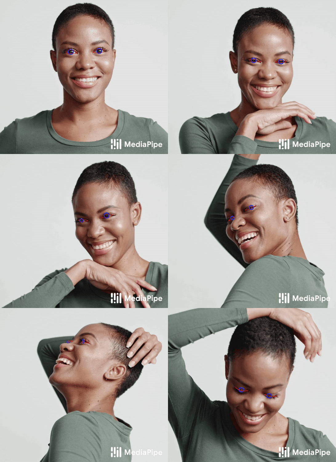
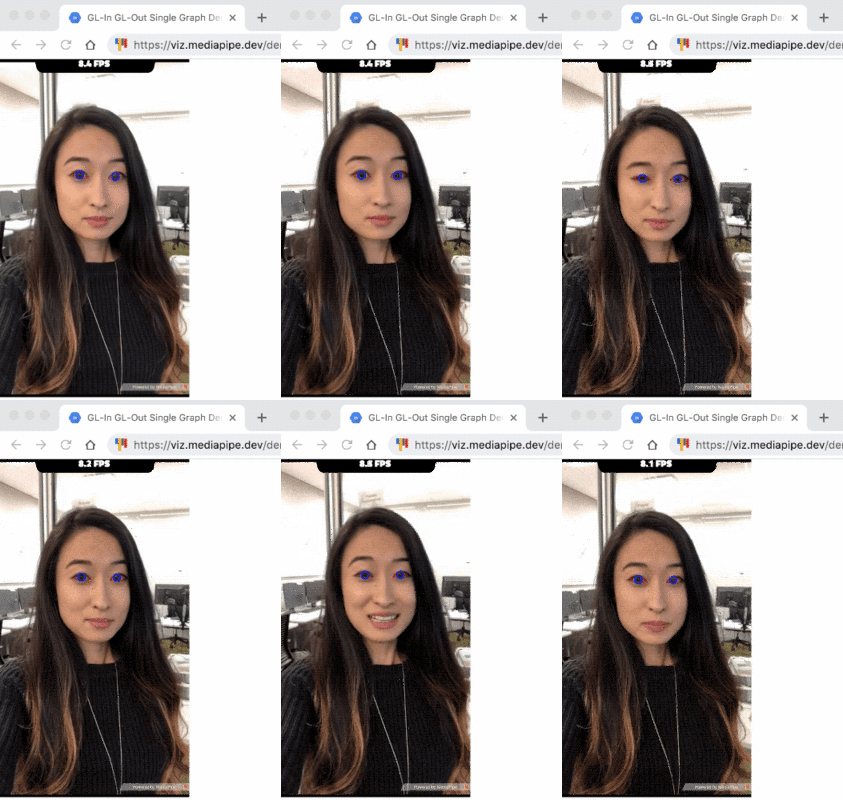
Examples of iris (blue) and eyelid (red) tracking.

To train the model from the cropped eye region, we manually annotated ~50k images, representing a variety of illumination conditions and head poses from geographically diverse regions, as shown below.

Eye region annotated with eyelid (red) and iris (blue) contours.
Cropped eye regions form the input to the model, which predicts landmarks via separate components.

Depth-from-Iris: Depth Estimation from a Single Image
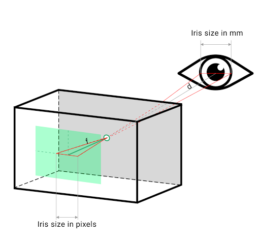
Our iris-tracking model is able to determine the metric distance of a subject to the camera with less than 10% error, without requiring any specialized hardware. This is done by relying on the fact that the horizontal iris diameter of the human eye remains roughly constant at 11.7±0.5 mm across a wide population [1, 2, 3, 4], along with some simple geometric arguments. For illustration, consider a pinhole camera model projecting onto a sensor of square pixels. The distance to a subject can be estimated from facial landmarks by using the focal length of the camera, which can be obtained using camera capture APIs or directly from the EXIF metadata of a captured image, along with other camera intrinsic parameters. Given the focal length, the distance from the subject to the camera is directly proportional to the physical size of the subject’s eye, as visualized below.

The distance of the subject (d) can be computed from the focal length (f) and the size of the iris using similar triangles.
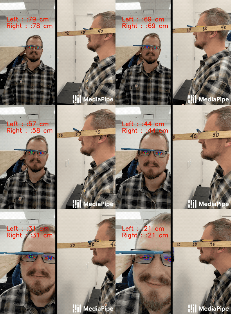
Left: MediaPipe Iris predicting metric distance in cm on a Pixel 2 from iris tracking alone, without the use of a depth sensor. Right: Ground-truth depth.

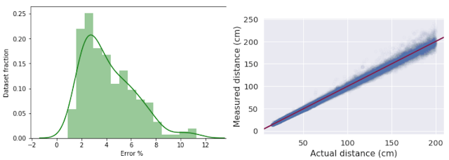
In order to quantify the accuracy of the method, we compared it to the depth sensor on an iPhone 11 by collecting front-facing, synchronized video and depth images on over 200 participants. We experimentally verified the error of the iPhone 11 depth sensor to be < 2% for distances up to 2 meters, using a laser ranging device. Our evaluation shows that our approach for depth estimation using iris size has a mean relative error of 4.3% and standard deviation of 2.4%. We tested our approach on participants with and without eyeglasses (not accounting for contact lenses on participants) and found that eyeglasses increase the mean relative error slightly to 4.8% (standard deviation 3.1%). We did not test this approach on participants with any eye diseases (like arcus senilis or pannus). Considering MediaPipe Iris requires no specialized hardware, these results suggest it may be possible to obtain metric depth from a single image on devices with a wide range of cost-points.

Histogram of estimation errors (left) and comparison of actual to estimated distance by iris (right).

Release of MediaPipe Iris
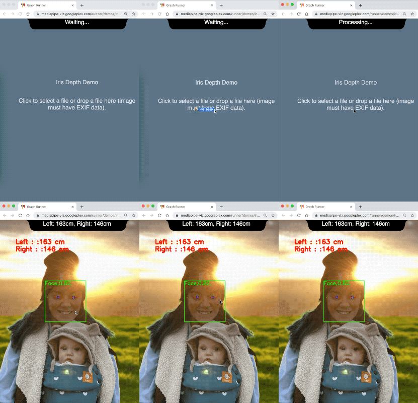
We are releasing the iris and depth estimation models as a cross-platform MediaPipe pipeline that can run on desktop, mobile and the web. As described in our recent Google Developer Blog post on MediaPipe on the web, we leverage WebAssembly and XNNPACK to run our Iris ML pipeline locally in the browser, without any data being sent to the cloud.

Using MediaPipe’s WASM stack, you can run the models locally in your browser! Left: Iris tracking. Right: Depth from Iris computed just from a photo with EXIF data. Iris tracking can be tried out here and iris depth measurements here.

Future Directions
We plan to extend our MediaPipe Iris model with even more stable tracking for lower error and deploy it for accessibility use cases. We strongly believe in sharing code that enables reproducible research, rapid experimentation, and development of new ideas in different areas. In our documentation and the accompanying Model Card, we detail the intended uses, limitations and model fairness to ensure that use of these models aligns with Google’s AI Principles. Note, that any form of surveillance or identification is explicitly out of scope and not enabled by this technology. We hope that providing this iris perception functionality to the wider research and development community will result in an emergence of creative use cases, stimulating responsible new applications and new research avenues.

For more ML solutions from MediaPipe, please see our solutions page and Google Developer blog for the latest updates.

Acknowledgements
We would like to thank Artsiom Ablavatski, Andrei Tkachenka, Buck Bourdon, Ivan Grishchenko and Gregory Karpiak for support in model evaluation and data collection; Yury Kartynnik, Valentin Bazarevsky, Artsiom Ablavatski for developing the mesh technology; Aliaksandr Shyrokau and the annotation team for their diligence to data preparation; Vidhya Navalpakkam, Tomer, Tomer Shekel, Kai Kohlhoff for their domain expertise, Fan Zhang, Esha Uboweja, Tyler Mullen, Michael Hays and Chuo-Ling Chang for help to integrate the model to MediaPipe; Matthias Grundmann, Florian Schroff and Ming Guang Yong for continuous help for building this technology.

Source: Google AI Blog


Live HDR+ and Dual Exposure Controls on Pixel 4 and 4a


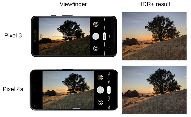
High dynamic range (HDR) imaging is a method for capturing scenes with a wide range of brightness, from deep shadows to bright highlights. On Pixel phones, the engine behind HDR imaging is HDR+ burst photography, which involves capturing a rapid burst of deliberately underexposed images, combining them, and rendering them in a way that preserves detail across the range of tones. Until recently, one challenge with HDR+ was that it could not be computed in real time (i.e., at 30 frames per second), which prevented the viewfinder from matching the final result. For example, bright white skies in the viewfinder might appear blue in the HDR+ result.

Starting with Pixel 4 and 4a, we have improved the viewfinder using a machine-learning-based approximation to HDR+, which we call Live HDR+. This provides a real-time preview of the final result, making HDR imaging more predictable. We also created dual exposure controls, which generalize the classic “exposure compensation” slider into two controls for separately adjusting the rendition of shadows and highlights. Together, Live HDR+ and dual exposure controls provide HDR imaging with real-time creative control.
Live HDR+ on Pixel 4 and 4a helps the user compose their shot with a WYSIWYG viewfinder that closely resembles the final result. You can see individual images here. Photos courtesy of Florian Kainz.
The HDR+ Look
When the user presses the shutter in the Pixel camera app, it captures 3-15 underexposed images. These images are aligned and merged to reduce noise in the shadows, producing a 14-bit intermediate “linear RGB image” with pixel values proportional to the scene brightness. What gives HDR+ images their signature look is the "tone mapping" of this image, reducing the range to 8 bits and making it suitable for display.

Consider the backlit photo of a motorcyclist, below. While the linear RGB image contains detail in both the dark motorcycle and bright sky, the dynamic range is too high to see it. The simplest method to reveal more detail is to apply a “global curve”, remapping all pixels with a particular brightness to some new value. However, for an HDR scene with details in both shadows and highlights, no single curve is satisfactory.
>Different ways to tone-map a linear RGB image. (a) The original, “un-tone-mapped” image. (b) Global curve optimizing for the sky. (c) Global curve optimizing for the subject. (d) HDR+, which preserves details everywhere. In the 2D histogram, brighter areas indicate where more pixels of a given input brightness are mapped to the same output. The overlapping shapes show that the relationship cannot be modeled using a single curve. Photo courtesy of Nicholas Wilson.
In contrast to applying a single curve, HDR+ uses a local tone mapping algorithm to ensure that the final result contains detail everywhere, while keeping edges and textures looking natural. Effectively, this applies a different curve to different regions, depending on factors such as overall brightness, local texture, and amount of noise. Unfortunately, HDR+ is too slow to run live in the viewfinder, requiring an alternative approach for Live HDR+.

Local Curve Approximation for Live HDR+
Using a single tone curve does not produce a satisfying result for the entire image — but how about for a small region? Consider the small red patch in the figure below. Although the patch includes both shadows and highlights, the relationship between input and output brightness follows a smooth curve. Furthermore, the curve varies gradually. For the blue patch, shifted ten pixels to the right, both the image content and curve are similar. But while the curve approximation works well for small patches, it breaks down for larger patches. For the larger yellow patch, the input/output relationship is more complicated, and not well approximated by a single curve.
(a) Input and HDR+ result. (b) The effect of HDR+ on a small patch (red) is approximately a smooth curve. (c) The relationship is nearly identical for the nearby blue patch. (d) However, if the patch is too big, a single curve will no longer provide a good fit.
To address this challenge, we divide the input image into “tiles” of size roughly equal to the red patch in the figure above, and approximate HDR+ using a curve for each tile. Since these curves vary gradually, blending between curves is a good way to approximate the optimal curve at any pixel. To render a pixel we apply the curves from each of the four nearest tiles, then blend the results according to the distances to the respective tile centers.

Compared to HDR+, this algorithm is particularly well suited for GPUs. Since the tone mapping of each pixel can be computed independently, the algorithm can also be parallelized. Moreover, the representation is memory-efficient: only a small number of tiles is enough to represent HDR+ local tone mapping for the viewfinder.

To compute local curves, we use a machine learning algorithm called HDRnet, a deep neural network that predicts, from a linear image, per-tile curves that approximate the HDR+ look of that image. It's also fast, due to its compact architecture and the way that low-resolution input images can be used to predict the curves for the high-resolution viewfinder. We train HDRnet on thousands of images to ensure it works well on all kinds of scenes.
HDRnet vs. HDR+ on a challenging scene with extreme brights and darks. The results are very similar at viewfinder resolution. Photo courtesy of Nicholas Wilson.
Dual Exposure Controls
HDR+ is designed to produce pleasing HDR images automatically, without the need for manual controls or post-processing. But sometimes the HDR+ rendition may not match the photographer’s artistic vision. While image editing tools are a partial remedy, HDR images can be challenging to edit, because some decisions are effectively baked into the final JPG. To maximize latitude for editing, it’s possible to save RAW images for each shot (an option in the app). However, this process takes the photographer out of the moment and requires expertise with RAW editing tools as well as additional storage.

Another approach to artistic control is to provide it live in the viewfinder. Many photographers are familiar with the exposure compensation slider, which brightens or darkens the image. But overall brightness is not expressive enough for HDR photography. At a minimum two controls are needed in order to control the highlights and shadows separately.

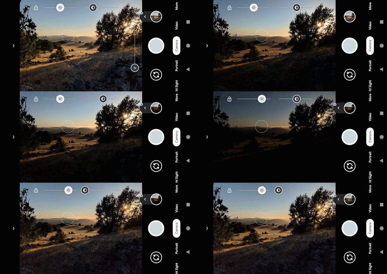
To address this, we introduce dual exposure controls. When the user taps on the Live HDR+ viewfinder, two sliders appear. The "Brightness" slider works like traditional exposure compensation, changing the overall exposure. This slider is used to recover more detail in bright skies, or intentionally blow out the background and make the subject more visible. The "Shadows" slider affects only dark areas — it operates by changing the tone mapping, not the exposure. This slider is most useful for high-contrast scenes, letting the user boost shadows to reveal details, or suppress them to create a silhouette.
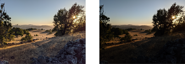
Screen capture of dual exposure controls in action on an outdoor HDR scene with HDR+ results below. You can see individual images here. Photos courtesy of Florian Kainz.
Here are some of the dramatic renditions we were able to achieve using dual exposure controls.
Different renditions using Dual Exposure Controls. You can see individual images here. Photo credits: Jiawen Chen, Florian Kainz, Alexander Schiffhauer.
Dual Exposure Controls gives you the flexibility to capture dramatically different versions of the same subject. They are not limited to tough HDR scenes, so don’t be afraid to experiment with different subjects and lighting. You may be surprised at how much these sliders will change how you shoot!

Acknowledgements
Live HDR+ and Dual Exposure Controls is the result of a collaboration between Google Research, Android, Hardware, and UX Design teams. Key contributors include: Francois Bleibel, Sean Callanan, Yulun Chang, Eric Chen, Michelle Chen, Kourosh Derakshan, Ryan Geiss, Zhijun He, Joy Hsu, Liz Koh, Marc Levoy, Chia-Kai Liang, Diane Liang, Timothy Lin, Gaurav Malik, Hossein Mohtasham, Nandini Mukherjee, Sushil Nath, Gabriel Nava, Karl Rasche, YiChang Shih, Daniel Solomon, Gary Sun, Kelly Tsai, Sung-fang Tsai, Ted Tsai, Ruben Velarde, Lida Wang, Tianfan Xue, Junlan Yang.

Source: Google AI Blog