Tag Archives: datasets

Introducing CVSS: A Massively Multilingual Speech-to-Speech Translation Corpus

Automatic translation of speech from one language to speech in another language, called speech-to-speech translation (S2ST), is important for breaking down the communication barriers between people speaking different languages. Conventionally, automatic S2ST systems are built with a cascade of automatic speech recognition (ASR), text-to-text machine translation (MT), and text-to-speech (TTS) synthesis sub-systems, so that the system overall is text-centric. Recently, work on S2ST that doesn’t rely on intermediate text representation is emerging, such as end-to-end direct S2ST (e.g., Translatotron) and cascade S2ST based on learned discrete representations of speech (e.g., Tjandra et al.). While early versions of such direct S2ST systems obtained lower translation quality compared to cascade S2ST models, they are gaining traction as they have the potential both to reduce translation latency and compounding errors, and to better preserve paralinguistic and non-linguistic information from the original speech, such as voice, emotion, tone, etc. However, such models usually have to be trained on datasets with paired S2ST data, but the public availability of such corpora is extremely limited.

To foster research on such a new generation of S2ST, we introduce a Common Voice-based Speech-to-Speech translation corpus, or CVSS, which includes sentence-level speech-to-speech translation pairs from 21 languages into English. Unlike existing public corpora, CVSS can be directly used for training such direct S2ST models without any extra processing. In “CVSS Corpus and Massively Multilingual Speech-to-Speech Translation”, we describe the dataset design and development, and demonstrate the effectiveness of the corpus through training of baseline direct and cascade S2ST models and showing performance of a direct S2ST model that approaches that of a cascade S2ST model.

Building CVSS
CVSS is directly derived from the CoVoST 2 speech-to-text (ST) translation corpus, which is further derived from the Common Voice speech corpus. Common Voice is a massively multilingual transcribed speech corpus designed for ASR in which the speech is collected by contributors reading text content from Wikipedia and other text corpora. CoVoST 2 further provides professional text translation for the original transcript from 21 languages into English and from English into 15 languages. CVSS builds on these efforts by providing sentence-level parallel speech-to-speech translation pairs from 21 languages into English (shown in the table below).

To facilitate research with different focuses, two versions of translation speech in English are provided in CVSS, both are synthesized using state-of-the-art TTS systems, with each version providing unique value that doesn’t exist in other public S2ST corpora:

  • CVSS-C: All the translation speech is in a single canonical speaker’s voice. Despite being synthetic, the speech is highly natural, clean, and consistent in speaking style. These properties ease the modeling of the target speech and enable trained models to produce high quality translation speech suitable for general user-facing applications where speech quality is of higher importance than accurately reproducing the speakers' voices.
  • CVSS-T: The translation speech captures the voice from the corresponding source speech. Each S2ST pair has a similar voice on the two sides, despite being in different languages. Because of this, the dataset is suitable for building models where accurate voice preservation is desired, such as for movie dubbing.

Together with the source speech, the two S2ST datasets contain 1,872 and 1,937 hours of speech, respectively.

Source
Language    
Code     Source
  speech (X)  
CVSS-C
  target speech (En)  
CVSS-T
  target speech (En)  
French fr 309.3 200.3 222.3
German de 226.5 137.0 151.2
Catalan ca 174.8 112.1 120.9
Spanish es 157.6 94.3 100.2
Italian it 73.9 46.5 49.2
Persian fa 58.8 29.9 34.5
Russian ru 38.7 26.9 27.4
Chinese zh 26.5 20.5 22.1
Portuguese     pt 20.0 10.4 11.8
Dutch nl 11.2 7.3 7.7
Estonian et 9.0 7.3 7.1
Mongolian mn 8.4 5.1 5.7
Turkish tr 7.9 5.4 5.7
Arabic ar 5.8 2.7 3.1
Latvian lv 4.9 2.6 3.1
Swedish sv 4.3 2.3 2.8
Welsh cy 3.6 1.9 2.0
Tamil ta 3.1 1.7 2.0
Indonesian id 3.0 1.6 1.7
Japanese ja 3.0 1.7 1.8
Slovenian sl 2.9 1.6 1.9
Total 1,153.2 719.1 784.2
Amount of source and target speech of each X-En pair in CVSS (hours).

In addition to translation speech, CVSS also provides normalized translation text matching the pronunciation in the translation speech (on numbers, currencies, acronyms, etc., see data samples below, e.g., where “100%” is normalized as “one hundred percent” or “King George II” is normalized as “king george the second”), which can benefit both model training as well as standardizing the evaluation.

CVSS is released under the Creative Commons Attribution 4.0 International (CC BY 4.0) license and it can be freely downloaded online.

Data Samples

Example 1:
Source audio (French)   
Source transcript (French)    Le genre musical de la chanson est entièrement le disco.
CVSS-C translation audio (English)   
CVSS-T translation audio (English)   
Translation text (English)    The musical genre of the song is 100% Disco.
Normalized translation text (English)        the musical genre of the song is one hundred percent disco
   
   
Example 2:
Source audio (Chinese)       
Source transcript (Chinese)        弗雷德里克王子,英国王室成员,为乔治二世之孙,乔治三世之幼弟。
CVSS-C translation audio (English)       
CVSS-T translation audio (English)       
Translation text (English)        Prince Frederick, member of British Royal Family, Grandson of King George II, brother of King George III.
Normalized translation text (English)        prince frederick member of british royal family grandson of king george the second brother of king george the third

Baseline Models
On each version of CVSS, we trained a baseline cascade S2ST model as well as two baseline direct S2ST models and compared their performance. These baselines can be used for comparison in future research.

Cascade S2ST: To build strong cascade S2ST baselines, we trained an ST model on CoVoST 2, which outperforms the previous states of the art by +5.8 average BLEU on all 21 language pairs (detailed in the paper) when trained on the corpus without using extra data. This ST model is connected to the same TTS models used for constructing CVSS to compose very strong cascade S2ST baselines (ST → TTS).

Direct S2ST: We built two baseline direct S2ST models using Translatotron and Translatotron 2. When trained from scratch with CVSS, the translation quality from Translatotron 2 (8.7 BLEU) approaches that of the strong cascade S2ST baseline (10.6 BLEU). Moreover, when both use pre-training the gap decreases to only 0.7 BLEU on ASR transcribed translation. These results verify the effectiveness of using CVSS to train direct S2ST models.

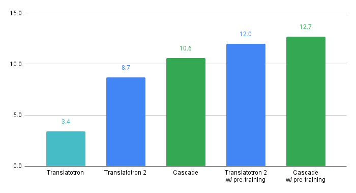
Translation quality of baseline direct and cascade S2ST models built on CVSS-C, measured by BLEU on ASR transcription from speech translation. The pre-training was done on CoVoST 2 without other extra data sets.

Conclusion
We have released two versions of multilingual-to-English S2ST datasets, CVSS-C and CVSS-T, each with about 1.9K hours of sentence-level parallel S2ST pairs, covering 21 source languages. The translation speech in CVSS-C is in a single canonical speaker’s voice, while the same in CVSS-T is in voices transferred from the source speech. Each of these datasets provides unique value not existing in other public S2ST corpora.

We built baseline multilingual direct S2ST models and cascade S2ST models on both datasets, which can be used for comparison in future works. To build strong cascade S2ST baselines, we trained an ST model on CoVoST 2, which outperforms the previous states of the art by +5.8 average BLEU when trained on the corpus without extra data. Nevertheless, the performance of the direct S2ST models approaches the strong cascade baselines when trained from scratch, and with only 0.7 BLEU difference on ASR transcribed translation when utilized pre-training. We hope this work helps accelerate the research on direct S2ST.

Acknowledgments
We acknowledge the volunteer contributors and the organizers of the Common Voice and LibriVox projects for their contribution and collection of recordings, the creators of Common Voice, CoVoST, CoVoST 2, Librispeech and LibriTTS corpora for their previous work. The direct contributors to the CVSS corpus and the paper include Ye Jia, Michelle Tadmor Ramanovich, Quan Wang, Heiga Zen. We also thank Ankur Bapna, Yiling Huang, Jason Pelecanos, Colin Cherry, Alexis Conneau, Yonghui Wu, Hadar Shemtov and Françoise Beaufays for helpful discussions and support.

Source: Google AI Blog


Training Machine Learning Models More Efficiently with Dataset Distillation

For a machine learning (ML) algorithm to be effective, useful features must be extracted from (often) large amounts of training data. However, this process can be made challenging due to the costs associated with training on such large datasets, both in terms of compute requirements and wall clock time. The idea of distillation plays an important role in these situations by reducing the resources required for the model to be effective. The most widely known form of distillation is model distillation (a.k.a. knowledge distillation), where the predictions of large, complex teacher models are distilled into smaller models.

An alternative option to this model-space approach is dataset distillation [1, 2], in which a large dataset is distilled into a synthetic, smaller dataset. Training a model with such a distilled dataset can reduce the required memory and compute. For example, instead of using all 50,000 images and labels of the CIFAR-10 dataset, one could use a distilled dataset consisting of only 10 synthesized data points (1 image per class) to train an ML model that can still achieve good performance on the unseen test set.

Top: Natural (i.e., unmodified) CIFAR-10 images. Bottom: Distilled dataset (1 image per class) on CIFAR-10 classification task. Using only these 10 synthetic images as training data, a model can achieve test set accuracy of ~51%.

In “Dataset Meta-Learning from Kernel Ridge Regression'', published in ICLR 2021, and “Dataset Distillation with Infinitely Wide Convolutional Networks”, presented at NeurIPS 2021, we introduce two novel dataset distillation algorithms, Kernel Inducing Points (KIP) and Label Solve (LS), which optimize datasets using the loss function arising from kernel regression (a classical machine learning algorithm that fits a linear model to features defined through a kernel). Applying the KIP and LS algorithms, we obtain very efficient distilled datasets for image classification, reducing the datasets to 1, 10, or 50 data points per class while still obtaining state-of-the-art results on a number of benchmark image classification datasets. Additionally, we are also excited to release our distilled datasets to benefit the wider research community.

Methodology
One of the key theoretical insights of deep neural networks (DNN) in recent years has been that increasing the width of DNNs results in more regular behavior that makes them easier to understand. As the width is taken to infinity, DNNs trained by gradient descent converge to the familiar and simpler class of models arising from kernel regression with respect to the neural tangent kernel (NTK), a kernel that measures input similarity by computing dot products of gradients of the neural network. Thanks to the Neural Tangents library, neural kernels for various DNN architectures can be computed in a scalable manner.

We utilized the above infinite-width limit theory of neural networks to tackle dataset distillation. Dataset distillation can be formulated as a two-stage optimization process: an “inner loop” that trains a model on learned data, and an “outer loop” that optimizes the learned data for performance on natural (i.e., unmodified) data. The infinite-width limit replaces the inner loop of training a finite-width neural network with a simple kernel regression. With the addition of a regularizing term, the kernel regression becomes a kernel ridge-regression (KRR) problem. This is a highly valuable outcome because the kernel ridge regressor (i.e., the predictor from the algorithm) has an explicit formula in terms of its training data (unlike a neural network predictor), which means that one can easily optimize the KRR loss function during the outer loop.

The original data labels can be represented by one-hot vectors, i.e., the true label is given a value of 1 and all other labels are given values of 0. Thus, an image of a cat would have the label “cat” assigned a 1 value, while the labels for “dog” and “horse” would be 0. The labels we use involve a subsequent mean-centering step, where we subtract the reciprocal of the number of classes from each component (so 0.1 for 10-way classification) so that the expected value of each label component across the dataset is normalized to zero.

While the labels for natural images appear in this standard form, the labels for our learned distilled datasets are free to be optimized for performance. Having obtained the kernel ridge regressor from the inner loop, the KRR loss function in the outer loop computes the mean-square error between the original labels of natural images and the labels predicted by the kernel ridge regressor. KIP optimizes the support data (images and possibly labels) by minimizing the KRR loss function through gradient-based methods. The Label Solve algorithm directly solves for the set of support labels that minimizes the KRR loss function, generating a unique dense label vector for each (natural) support image.

Example of labels obtained by label solving. Left and Middle: Sample images with possible labels listed below. The raw, one-hot label is shown in blue and the final LS generated dense label is shown in orange. Right: The covariance matrix between original labels and learned labels. Here, 500 labels were distilled from the CIFAR-10 dataset. A test accuracy of 69.7% is achieved using these labels for kernel ridge-regression.

Distributed Computation
For simplicity, we focus on architectures that consist of convolutional neural networks with pooling layers. Specifically, we focus on the so-called “ConvNet” architecture and its variants because it has been featured in other dataset distillation studies. We used a slightly modified version of ConvNet that has a simple architecture given by three blocks of convolution, ReLu, and 2x2 average pooling and then a final linear readout layer, with an additional 3x3 convolution and ReLu layer prepended (see our GitHub for precise details).

ConvNet architecture used in DC/DSA. Ours has an additional 3x3 Conv and ReLu prepended.

To compute the neural kernels needed in our work, we used the Neural Tangents library.

The first stage of this work, in which we applied KRR, focused on fully-connected networks, whose kernel elements are cheap to compute. But a hurdle facing neural kernels for models with convolutional layers plus pooling is that the computation of each kernel element between two images scales as the square of the number of input pixels (due to the capturing of pixel-pixel correlations by the kernel). So, for the second stage of this work, we needed to distribute the computation of the kernel elements and their gradients across many devices.

Distributed computation for large scale metalearning.

We invoke a client-server model of distributed computation in which a server distributes independent workloads to a large pool of client workers. A key part of this is to divide the backpropagation step in a way that is computationally efficient (explained in detail in the paper).

We accomplish this using the open-source tools Courier (part of DeepMind’s Launchpad), which allows us to distribute computations across GPUs working in parallel, and JAX, for which novel usage of the jax.vjp function enables computationally efficient gradients. This distributed framework allows us to utilize hundreds of GPUs per distillation of the dataset, for both the KIP and LS algorithms. Given the compute required for such experiments, we are releasing our distilled datasets to benefit the wider research community.

Examples
Our first set of distilled images above used KIP to distill CIFAR-10 down to 1 image per class while keeping the labels fixed. Next, in the below figure, we compare the test accuracy of training on natural MNIST images, KIP distilled images with labels fixed, and KIP distilled images with labels optimized. We highlight that learning the labels provides an effective, albeit mysterious benefit to distilling datasets. Indeed the resulting set of images provides the best test performance (for infinite-width networks) despite being less interpretable.

MNIST dataset distillation with trainable and non-trainable labels. Top: Natural MNIST data. Middle: Kernel Inducing Point distilled data with fixed labels. Bottom: Kernel Inducing Point distilled data with learned labels.

Results
Our distilled datasets achieve state-of-the-art performance on benchmark image classification datasets, improving performance beyond previous state-of-the-art models that used convolutional architectures, Dataset Condensation (DC) and Dataset Condensation with Differentiable Siamese Augmentation (DSA). In particular, for CIFAR-10 classification tasks, a model trained on a dataset consisting of only 10 distilled data entries (1 image / class, 0.02% of the whole dataset) achieves a 64% test set accuracy. Here, learning labels and an additional image preprocessing step leads to a significant increase in performance beyond the 50% test accuracy shown in our first figure (see our paper for details). With 500 images (50 images / class, 1% of the whole dataset), the model reaches 80% test set accuracy. While these numbers are with respect to neural kernels (using the KRR infinite width limit), these distilled datasets can be used to train finite-width neural networks as well. In particular, for 10 data points on CIFAR-10, a finite-width ConvNet neural network achieves 50% test accuracy with 10 images and 68% test accuracy using 500 images, which are still state-of-the-art results. We provide a simple Colab notebook demonstrating this transfer to a finite-width neural network.

Dataset distillation using Kernel Inducing Points (KIP) with a convolutional architecture outperforms prior state-of-the-art models (DC/DSA) on all benchmark settings on image classification tasks. Label Solve (LS, middle columns) while only distilling information in the labels could often (e.g. CIFAR-10 10, 50 data points per class) outperform prior state-of-the-art models as well.

In some cases, our learned datasets are more effective than a natural dataset one hundred times larger in size.

Conclusion
We believe that our work on dataset distillation opens up many interesting future directions. For instance, our algorithms KIP and LS have demonstrated the effectiveness of using learned labels, an area that remains relatively underexplored. Furthermore, we expect that utilizing efficient kernel approximation methods can help to reduce computational burden and scale up to larger datasets. We hope this work encourages researchers to explore other applications of dataset distillation, including neural architecture search and continual learning, and even potential applications to privacy.

Anyone interested in the KIP and LS learned datasets for further analysis is encouraged to check out our papers [ICLR 2021, NeurIPS 2021] and open-sourced code and datasets available on Github.

Acknowledgement
This project was done in collaboration with Zhourong Chen, Roman Novak and Lechao Xiao. We would like to acknowledge special thanks to Samuel S. Schoenholz, who proposed and helped develop the overall strategy for our distributed KIP learning methodology.


1Now at DeepMind.  

Source: Google AI Blog


RLDS: An Ecosystem to Generate, Share, and Use Datasets in Reinforcement Learning

Most reinforcement learning (RL) and sequential decision making algorithms require an agent to generate training data through large amounts of interactions with their environment to achieve optimal performance. This is highly inefficient, especially when generating those interactions is difficult, such as collecting data with a real robot or by interacting with a human expert. This issue can be mitigated by reusing external sources of knowledge, for example, the RL Unplugged Atari dataset, which includes data of a synthetic agent playing Atari games.

However, there are very few of these datasets and a variety of tasks and ways of generating data in sequential decision making (e.g., expert data or noisy demonstrations, human or synthetic interactions, etc.), making it unrealistic and not even desirable for the whole community to work on a small number of representative datasets because these will never be representative enough. Moreover, some of these datasets are released in a form that only works with certain algorithms, which prevents researchers from reusing this data. For example, rather than including the sequence of interactions with the environment, some datasets provide a set of random interactions, making it impossible to reconstruct the temporal relation between them, while others are released in slightly different formats, which can introduce subtle bugs that are very difficult to identify.

In this context, we introduce Reinforcement Learning Datasets (RLDS), and release a suite of tools for recording, replaying, manipulating, annotating and sharing data for sequential decision making, including offline RL, learning from demonstrations, or imitation learning. RLDS makes it easy to share datasets without any loss of information (e.g., keeping the sequence of interactions instead of randomizing them) and to be agnostic to the underlying original format, enabling users to quickly test new algorithms on a wider range of tasks. Additionally, RLDS provides tools for collecting data generated by either synthetic agents (EnvLogger) or humans (RLDS Creator), as well as for inspecting and manipulating the collected data. Ultimately, integration with TensorFlow Datasets (TFDS) facilitates the sharing of RL datasets with the research community.

With RLDS, users can record interactions between an agent and an environment in a lossless and standard format. Then, they can use and transform this data to feed different RL or Sequential Decision Making algorithms, or to perform data analysis.

Dataset Structure
Algorithms in RL, offline RL, or imitation learning may consume data in very different formats, and, if the format of the dataset is unclear, it's easy to introduce bugs caused by misinterpretations of the underlying data. RLDS makes the data format explicit by defining the contents and the meaning of each of the fields of the dataset, and provides tools to re-align and transform this data to fit the format required by any algorithm implementation. In order to define the data format, RLDS takes advantage of the inherently standard structure of RL datasets — i.e., sequences (episodes) of interactions (steps) between agents and environments, where agents can be, for example, rule-based/automation controllers, formal planners, humans, animals, or a combination of these. Each of these steps contains the current observation, the action applied to the current observation, the reward obtained as a result of applying action, and the discount obtained together with reward. Steps also include additional information to indicate whether the step is the first or last of the episode, or if the observation corresponds to a terminal state. Each step and episode may also contain custom metadata that can be used to store environment-related or model-related data.

Producing the Data
Researchers produce datasets by recording the interactions with an environment made by any kind of agent. To maintain its usefulness, raw data is ideally stored in a lossless format by recording all the information that is produced, keeping the temporal relation between the data items (e.g., ordering of steps and episodes), and without making any assumption on how the dataset is going to be used in the future. For this, we release EnvLogger, a software library to log agent-environment interactions in an open format.

EnvLogger is an environment wrapper that records agent–environment interactions and saves them in long-term storage. Although EnvLogger is seamlessly integrated in the RLDS ecosystem, we designed it to be usable as a stand-alone library for greater modularity.

As in most machine learning settings, collecting human data for RL is a time consuming and labor intensive process. The common approach to address this is to use crowd-sourcing, which requires user-friendly access to environments that may be difficult to scale to large numbers of participants. Within the RLDS ecosystem, we release a web-based tool called RLDS Creator, which provides a universal interface to any human-controllable environment through a browser. Users can interact with the environments, e.g., play the Atari games online, and the interactions are recorded and stored such that they can be loaded back later using RLDS for analysis or to train agents.

Sharing the Data
Datasets are often onerous to produce, and sharing with the wider research community not only enables reproducibility of former experiments, but also accelerates research as it makes it easier to run and validate new algorithms on a range of scenarios. For that purpose, RLDS is integrated with TensorFlow Datasets (TFDS), an existing library for sharing datasets within the machine learning community. Once a dataset is part of TFDS, it is indexed in the global TFDS catalog, making it accessible to any researcher by using tfds.load(name_of_dataset), which loads the data either in Tensorflow or in Numpy formats.

TFDS is independent of the underlying format of the original dataset, so any existing dataset with RLDS-compatible format can be used with RLDS, even if it was not originally generated with EnvLogger or RLDS Creator. Also, with TFDS, users keep ownership and full control over their data and all datasets include a citation to credit the dataset authors.

Consuming the Data
Researchers can use the datasets in order to analyze, visualize or train a variety of machine learning algorithms, which, as noted above, may consume data in different formats than how it has been stored. For example, some algorithms, like R2D2 or R2D3, consume full episodes; others, like Behavioral Cloning or ValueDice, consume batches of randomized steps. To enable this, RLDS provides a library of transformations for RL scenarios. These transformations have been optimized, taking into account the nested structure of the RL datasets, and they include auto-batching to accelerate some of these operations. Using those optimized transformations, RLDS users have full flexibility to easily implement some high level functionalities, and the pipelines developed are reusable across RLDS datasets. Example transformations include statistics across the full dataset for selected step fields (or sub-fields) or flexible batching respecting episode boundaries. You can explore the existing transformations in this tutorial and see more complex real examples in this Colab.

Available Datasets
At the moment, the following datasets (compatible with RLDS) are in TFDS:

Our team is committed to quickly expanding this list in the near future and external contributions of new datasets to RLDS and TFDS are welcomed.

Conclusion
The RLDS ecosystem not only improves reproducibility of research in RL and sequential decision making problems, but also enables new research by making it easier to share and reuse data. We hope the capabilities offered by RLDS will initiate a trend of releasing structured RL datasets, holding all the information and covering a wider range of agents and tasks.

Acknowledgements
Besides the authors of this post, this work has been done by Google Research teams in Paris and Zurich in Collaboration with Deepmind. In particular by Sertan Girgin, Damien Vincent, Hanna Yakubovich, Daniel Kenji Toyama, Anita Gergely, Piotr Stanczyk, Raphaël Marinier, Jeremiah Harmsen, Olivier Pietquin and Nikola Momchev. We also want to thank the collaboration of other engineers and researchers who provided feedback and contributed to the project. In particular, George Tucker, Sergio Gomez, Jerry Li, Caglar Gulcehre, Pierre Ruyssen, Etienne Pot, Anton Raichuk, Gabriel Dulac-Arnold, Nino Vieillard, Matthieu Geist, Alexandra Faust, Eugene Brevdo, Tom Granger, Zhitao Gong, Toby Boyd and Tom Small.

Source: Google AI Blog


GoEmotions: A Dataset for Fine-Grained Emotion Classification

Emotions are a key aspect of social interactions, influencing the way people behave and shaping relationships. This is especially true with language — with only a few words, we're able to express a wide variety of subtle and complex emotions. As such, it’s been a long-term goal among the research community to enable machines to understand context and emotion, which would, in turn, enable a variety of applications, including empathetic chatbots, models to detect harmful online behavior, and improved customer support interactions.

In the past decade, the NLP research community has made available several datasets for language-based emotion classification. The majority of those are constructed manually and cover targeted domains (news headlines, movie subtitles, and even fairy tales) but tend to be relatively small, or focus only on the six basic emotions (anger, surprise, disgust, joy, fear, and sadness) that were proposed in 1992. While these emotion datasets enabled initial explorations into emotion classification, they also highlighted the need for a large-scale dataset over a more extensive set of emotions that could facilitate a broader scope of future potential applications.

In “GoEmotions: A Dataset of Fine-Grained Emotions”, we describe GoEmotions, a human-annotated dataset of 58k Reddit comments extracted from popular English-language subreddits and labeled with 27 emotion categories . As the largest fully annotated English language fine-grained emotion dataset to date, we designed the GoEmotions taxonomy with both psychology and data applicability in mind. In contrast to the basic six emotions, which include only one positive emotion (joy), our taxonomy includes 12 positive, 11 negative, 4 ambiguous emotion categories and 1 “neutral”, making it widely suitable for conversation understanding tasks that require a subtle differentiation between emotion expressions.

We are releasing the GoEmotions dataset along with a detailed tutorial that demonstrates the process of training a neural model architecture (available on TensorFlow Model Garden) using GoEmotions and applying it for the task of suggesting emojis based on conversational text. In the GoEmotions Model Card we explore additional uses for models built with GoEmotions, as well as considerations and limitations for using the data.

This text expresses several emotions at once, including excitement, approval and gratitude.
This text expresses relief, a complex emotion conveying both positive and negative sentiment.
This text conveys remorse, a complex emotion that is expressed frequently but is not captured by simple models of emotion.

Building the Dataset
Our goal was to build a large dataset, focused on conversational data, where emotion is a critical component of the communication. Because the Reddit platform offers a large, publicly available volume of content that includes direct user-to-user conversation, it is a valuable resource for emotion analysis. So, we built GoEmotions using Reddit comments from 2005 (the start of Reddit) to January 2019, sourced from subreddits with at least 10k comments, excluding deleted and non-English comments.

To enable building broadly representative emotion models, we applied data curation measures to ensure the dataset does not reinforce general, nor emotion-specific, language biases. This was particularly important because Reddit has a known demographic bias leaning towards young male users, which is not reflective of a globally diverse population. The platform also introduces a skew towards toxic, offensive language. To address these concerns, we identified harmful comments using predefined terms for offensive/adult and vulgar content, and for identity and religion, which we used for data filtering and masking. We additionally filtered the data to reduce profanity, limit text length, and balance for represented emotions and sentiments. To avoid over-representation of popular subreddits and to ensure the comments also reflect less active subreddits, we also balanced the data among subreddit communities.

We created a taxonomy seeking to jointly maximize three objectives: (1) provide the greatest coverage of the emotions expressed in Reddit data; (2) provide the greatest coverage of types of emotional expressions; and (3) limit the overall number of emotions and their overlap. Such a taxonomy allows data-driven fine-grained emotion understanding, while also addressing potential data sparsity for some emotions.

Establishing the taxonomy was an iterative process to define and refine the emotion label categories. During the data labeling stages, we considered a total of 56 emotion categories. From this sample, we identified and removed emotions that were scarcely selected by raters, had low interrater agreement due to similarity to other emotions, or were difficult to detect from text. We also added emotions that were frequently suggested by raters and were well represented in the data. Finally, we refined emotion category names to maximize interpretability, leading to high interrater agreement, with 94% of examples having at least two raters agreeing on at least 1 emotion label.

The published GoEmotions dataset includes the taxonomy presented below, and was fully collected through a final round of data labeling where both the taxonomy and rating standards were pre-defined and fixed.

GoEmotions taxonomy: Includes 28 emotion categories, including “neutral”.

Data Analysis and Results
Emotions are not distributed uniformly in the GoEmotions dataset. Importantly, the high frequency of positive emotions reinforces our motivation for a more diverse emotion taxonomy than that offered by the canonical six basic emotions.

To validate that our taxonomic choices match the underlying data, we conduct principal preserved component analysis (PPCA), a method used to compare two datasets by extracting linear combinations of emotion judgments that exhibit the highest joint variability across two sets of raters. It therefore helps us uncover dimensions of emotion that have high agreement across raters. PPCA was used before to understand principal dimensions of emotion recognition in video and speech, and we use it here to understand the principal dimensions of emotion in text.

We find that each component is significant (with p-values < 1.5e-6 for all dimensions), indicating that each emotion captures a unique part of the data. This is not trivial, since in previous work on emotion recognition in speech, only 12 out of 30 dimensions of emotion were found to be significant.

We examine the clustering of the defined emotions based on correlations among rater judgments. With this approach, two emotions will cluster together when they are frequently co-selected by raters. We find that emotions that are related in terms of their sentiment (negative, positive and ambiguous) cluster together, despite no predefined notion of sentiment in our taxonomy, indicating the quality and consistency of the ratings. For example, if one rater chose "excitement" as a label for a given comment, it is more likely that another rater would choose a correlated sentiment, such as "joy", rather than, say, "fear". Perhaps surprisingly, all ambiguous emotions clustered together, and they clustered more closely with positive emotions.

Similarly, emotions that are related in terms of their intensity, such as joy and excitement, nervousness and fear, sadness and grief, annoyance and anger, are also closely correlated.

Our paper provides additional analyses and modeling experiments using GoEmotions.

Future Work: Alternatives to Human-Labeling
While GoEmotions offers a large set of human-annotated emotion data, additional emotion datasets exist that use heuristics for automatic weak-labeling. The dominant heuristic uses emotion-related Twitter tags as emotion categories, which allows one to inexpensively generate large datasets. But this approach is limited for multiple reasons: the language used on Twitter is demonstrably different than many other language domains, thus limiting the applicability of the data; tags are human generated, and, when used directly, are prone to duplication, overlap, and other taxonomic inconsistencies; and the specificity of this approach to Twitter limits its applications to other language corpora.

We propose an alternative, and more easily available heuristic in which emojis embedded in user conversation serve as a proxy for emotion categories. This approach can be applied to any language corpora containing a reasonable occurence of emojis, including many that are conversational. Because emojis are more standardized and less sparse than Twitter-tags, they present fewer inconsistencies.

Note that both of the proposed approaches — using Twitter tags and using emojis — are not directly aimed at emotion understanding, but rather at variants of conversational expression. For example, in the conversation below, ? conveys gratitude, ? conveys a celebratory expression, and ? is a literal replacement for ‘present’. Similarly, while many emojis are associated with emotion-related expressions, emotions are subtle and multi-faceted, and in many cases no one emoji can truly capture the full complexity of an emotion. Moreover, emojis capture varying expressions beyond emotions. For these reasons, we consider them as expressions rather than emotions.

This type of data can be valuable for building expressive conversational agents, as well as for suggesting contextual emojis, and is a particularly interesting area of future work.

Conclusion
The GoEmotions dataset provides a large, manually annotated, dataset for fine-grained emotion prediction. Our analysis demonstrates the reliability of the annotations and high coverage of the emotions expressed in Reddit comments. We hope that GoEmotions will be a valuable resource to language-based emotion researchers, and will allow practitioners to build creative emotion-driven applications, addressing a wide range of user emotions.

Acknowledgements
This blog presents research done by Dora Demszky (while interning at Google), Dana Alon (previously Movshovitz-Attias), Jeongwoo Ko, Alan Cowen, Gaurav Nemade, and Sujith Ravi. We thank Peter Young for his infrastructure and open sourcing contributions. We thank Erik Vee, Ravi Kumar, Andrew Tomkins, Patrick Mcgregor, and the Learn2Compress team for support and sponsorship of this research project.

Source: Google AI Blog


Announcing WIT: A Wikipedia-Based Image-Text Dataset

Multimodal visio-linguistic models rely on rich datasets in order to model the relationship between images and text. Traditionally, these datasets have been created by either manually captioning images, or crawling the web and extracting the alt-text as the caption. While the former approach tends to result in higher quality data, the intensive manual annotation process limits the amount of data that can be created. On the other hand, the automated extraction approach can lead to bigger datasets, but these require either heuristics and careful filtering to ensure data quality or scaling-up models to achieve strong performance. An additional shortcoming of existing datasets is the dearth of coverage in non-English languages. This naturally led us to ask: Can one overcome these limitations and create a high-quality, large-sized, multilingual dataset with a variety of content?

Today we introduce the Wikipedia-Based Image Text (WIT) Dataset, a large multimodal dataset, created by extracting multiple different text selections associated with an image from Wikipedia articles and Wikimedia image links. This was accompanied by rigorous filtering to only retain high quality image-text sets. As detailed in “WIT: Wikipedia-based Image Text Dataset for Multimodal Multilingual Machine Learning”, presented at SIGIR ‘21, this resulted in a curated set of 37.5 million entity-rich image-text examples with 11.5 million unique images across 108 languages. The WIT dataset is available for download and use under the Creative Commons license. We are also excited to announce that we are hosting a competition with the WIT dataset in Kaggle in collaboration with Wikimedia Research and other external collaborators.

Dataset   Images     Text     Contextual Text     Languages  
Flickr30K 32K 158K - < 8
SBU Captions     1M 1M - 1
MS-COCO 330K 1.5M - < 4; 7 (test only)
CC-3M
CC-12M
3.3M
12M
3.3M
12M
-
-
1
1
WIT 11.5M 37.5M ~119M 108
WIT’s increased language coverage and larger size relative to previous datasets.

The unique advantages of the WIT dataset are:

  1. Size: WIT is the largest multimodal dataset of image-text examples that is publicly available.
  2. Multilingual: With 108 languages, WIT has 10x or more languages than any other dataset.
  3. Contextual information: Unlike typical multimodal datasets, which have only one caption per image, WIT includes many page-level and section-level contextual information.
  4. Real world entities: Wikipedia, being a broad knowledge-base, is rich with real world entities that are represented in WIT.
  5. Challenging test set: In our recent work accepted at EMNLP, all state-of-the-art models demonstrated significantly lower performance on WIT vs. traditional evaluation sets (e.g., ~30 point drop in recall).

Generating the Dataset
The main goal of WIT was to create a large dataset without sacrificing on quality or coverage of concepts. Thus, we started by leveraging the largest online encyclopedia available today: Wikipedia.

For an example of the depth of information available, consider the Wikipedia page for Half Dome (Yosemite National Park, CA). As shown below, the article has numerous interesting text captions and relevant contextual information for the image, such as the page title, main page description, and other contextual information and metadata.

Example wikipedia page with various image-associated text selections and contexts we can extract. From the Wikipedia page for Half Dome : Photo by DAVID ILIFF. License: CC BY-SA 3.0.
Example of the Wikipedia page for this specific image of Half Dome. From the Wikipedia page for Half Dome : Photo by DAVID ILIFF. License: CC BY-SA 3.0.

We started by selecting Wikipedia pages that have images, then extracted various image-text associations and surrounding contexts. To further refine the data, we performed a rigorous filtering process to ensure data quality. This included text-based filtering to ensure caption availability, length and quality (e.g., by removing generic default filler text); image-based filtering to ensure each image is a certain size with permissible licensing; and finally, image-and-text-entity–based filtering to ensure suitability for research (e.g., excluding those classified as hate speech). We further randomly sampled image-caption sets for evaluation by human editors, who overwhelmingly agreed that 98% of the samples had good image-caption alignment.

Highly Multilingual
With data in 108 languages, WIT is the first large-scale, multilingual, multimodal dataset.

# of Image-Text Sets   Unique Languages   # of Images   Unique Languages  
> 1M 9 > 1M 6
500K - 1M 10 500K - 1M 12
  100K - 500K   36   100K - 500K   35
50K - 100K 15 50K - 100K 17
14K - 50K 38 13K - 50K 38
WIT: coverage statistics across languages.
Example of an image that is present in more than a dozen Wikipedia pages across >12 languages. From the Wikipedia page for Wolfgang Amadeus Mozart.

The First Contextual Image-Text Dataset
Most multimodal datasets only offer a single text caption (or multiple versions of a similar caption) for the given image. WIT is the first dataset to provide contextual information, which can help researchers model the effect of context on image captions as well as the choice of images.

WIT dataset example showing image-text data and additional contextual information.

In particular, key textual fields of WIT that may be useful for research include:

  • Text captions: WIT offers three different kinds of image captions. This includes the (potentially context influenced) “Reference description”, the (likely context independent) “Attribution description” and “Alt-text description”.
  • Contextual information: This includes the page title, page description, URL and local context about the Wikipedia section including the section title and text.

WIT has broad coverage across these different fields, as shown below.

Image-Text Fields of WIT     Train Val Test Total / Unique
Rows / Tuples   37.1M     261.8K     210.7K   37.6M
Unique Images 11.4M 58K 57K 11.5M
Reference Descriptions 16.9M 150K 104K   17.2M / 16.7M  
Attribution Descriptions 34.8M 193K 200K 35.2M / 10.9M
Alt-Text 5.3M 29K 29K 5.4M / 5.3M
Context Texts - - - 119.8M
Key fields of WIT include both text captions and contextual information.

A High-Quality Training Set and a Challenging Evaluation Benchmark
The broad coverage of diverse concepts in Wikipedia means that the WIT evaluation sets serve as a challenging benchmark, even for state-of-the-art models. We found that for image-text retrieval, the mean recall scores for traditional datasets were in the 80s, whereas for the WIT test set, it was in the 40s for well-resourced languages and in the 30s for the under-resourced languages. We hope this in turn can help researchers to build stronger, more robust models.

WIT Dataset and Competition with Wikimedia and Kaggle
Additionally, we are happy to announce that we are partnering with Wikimedia Research and a few external collaborators to organize a competition with the WIT test set. We are hosting this competition in Kaggle. The competition is an image-text retrieval task. Given a set of images and text captions, the task is to retrieve the appropriate caption(s) for each image.

To enable research in this area, Wikipedia has kindly made available images at 300-pixel resolution and a Resnet-50–based image embeddings for most of the training and the test dataset. Kaggle will be hosting all this image data in addition to the WIT dataset itself and will provide colab notebooks. Further, the competitors will have access to a discussion forum in Kaggle in order to share code and collaborate. This enables anyone interested in multimodality to get started and run experiments easily. We are excited and looking forward to what will result from the WIT dataset and the Wikipedia images in the Kaggle platform.

Conclusion
We believe that the WIT dataset will aid researchers in building better multimodal multilingual models and in identifying better learning and representation techniques, ultimately leading to improved Machine Learning models in real-world tasks over visio-linguistic data. For any questions, please contact [email protected]. We would love to hear about how you are using the WIT dataset.

Acknowledgements
We would like to thank our co-authors in Google Research: Jiecao Chen, Michael Bendersky and Marc Najork. We thank Beer Changpinyo, Corinna Cortes, Joshua Gang, Chao Jia, Ashwin Kakarla, Mike Lee, Zhen Li, Piyush Sharma, Radu Soricut, Ashish Vaswani, Yinfei Yang, and our reviewers for their insightful feedback and comments.

We thank Miriam Redi and Leila Zia from Wikimedia Research for collaborating with us on the competition and providing image pixels and image embedding data. We thank Addison Howard and Walter Reade for helping us host this competition in Kaggle. We also thank Diane Larlus (Naver Labs Europe (NLE)), Yannis Kalantidis (NLE), Stéphane Clinchant (NLE), Tiziano Piccardi Ph.D. student at EPFL, Lucie-Aimée Kaffee PhD student at University of Southampton and Yacine Jernite (Hugging Face) for their valuable contribution towards the competition.

Source: Google AI Blog


The C4_200M Synthetic Dataset for Grammatical Error Correction

Grammatical error correction (GEC) attempts to model grammar and other types of writing errors in order to provide grammar and spelling suggestions, improving the quality of written output in documents, emails, blog posts and even informal chats. Over the past 15 years, there has been a substantial improvement in GEC quality, which can in large part be credited to recasting the problem as a "translation" task. When introduced in Google Docs, for example, this approach resulted in a significant increase in the number of accepted grammar correction suggestions.

One of the biggest challenges for GEC models, however, is data sparsity. Unlike other natural language processing (NLP) tasks, such as speech recognition and machine translation, there is very limited training data available for GEC, even for high-resource languages like English. A common remedy for this is to generate synthetic data using a range of techniques, from heuristic-based random word- or character-level corruptions to model-based approaches. However, such methods tend to be simplistic and do not reflect the true distribution of error types from actual users.

In “Synthetic Data Generation for Grammatical Error Correction with Tagged Corruption Models”, presented at the EACL 16th Workshop on Innovative Use of NLP for Building Educational Applications, we introduce tagged corruption models. Inspired by the popular back-translation data synthesis technique for machine translation, this approach enables the precise control of synthetic data generation, ensuring diverse outputs that are more consistent with the distribution of errors seen in practice. We used tagged corruption models to generate a new 200M sentence dataset, which we have released in order to provide researchers with realistic pre-training data for GEC. By integrating this new dataset into our training pipeline, we were able to significantly improve on GEC baselines.

Tagged Corruption Models
The idea behind applying a conventional corruption model to GEC is to begin with a grammatically correct sentence and then to “corrupt” it by adding errors. A corruption model can be easily trained by switching the source and target sentences in existing GEC datasets, a method that previous studies have shown that can be very effective for generating improved GEC datasets.

A conventional corruption model generates an ungrammatical sentence (red) given a clean input sentence (green).

The tagged corruption model that we propose builds on this idea by taking a clean sentence as input along with an error type tag that describes the kind of error one wishes to reproduce. It then generates an ungrammatical version of the input sentence that contains the given error type. Choosing different error types for different sentences increases the diversity of corruptions compared to a conventional corruption model.

Tagged corruption models generate corruptions (red) for the clean input sentence (green) depending on the error type tag. A determiner error may lead to dropping the “a”, whereas a noun-inflection error may produce the incorrect plural “sheeps”.

To use this model for data generation we first randomly selected 200M clean sentences from the C4 corpus, and assigned an error type tag to each sentence such that their relative frequencies matched the error type tag distribution of the small development set BEA-dev. Since BEA-dev is a carefully curated set that covers a wide range of different English proficiency levels, we expect its tag distribution to be representative for writing errors found in the wild. We then used a tagged corruption model to synthesize the source sentence.

Synthetic data generation with tagged corruption models. The clean C4 sentences (green) are paired with the corrupted sentences (red) in the synthetic GEC training corpus. The corrupted sentences are generated using a tagged corruption model by following the error type frequencies in the development set (bar chart).

Results
In our experiments, tagged corruption models outperformed untagged corruption models on two standard development sets (CoNLL-13 and BEA-dev) by more than three F0.5-points (a standard metric in GEC research that combines precision and recall with more weight on precision), advancing the state-of-the-art on the two widely used academic test sets, CoNLL-14 and BEA-test.

In addition, the use of tagged corruption models not only yields gains on standard GEC test sets, it is also able to adapt GEC systems to the proficiency levels of users. This could be useful, for example, because the error tag distribution for native English writers often differs significantly from the distributions for non-native English speakers. For example, native speakers tend to make more punctuation and spelling mistakes, whereas determiner errors (e.g., missing or superfluous articles, like “a”, “an” or “the”) are more common in text from non-native writers.

Conclusion
Neural sequence models are notoriously data-hungry, but the availability of annotated training data for grammatical error correction is rare. Our new C4_200M corpus is a synthetic dataset containing diverse grammatical errors, which yields state-of-the-art performance when used to pre-train GEC systems. By releasing the dataset we hope to provide GEC researchers with a valuable resource to train strong baseline systems.

Source: Google AI Blog


Mapping Africa’s Buildings with Satellite Imagery

An accurate record of building footprints is important for a range of applications, from population estimation and urban planning to humanitarian response and environmental science. After a disaster, such as a flood or an earthquake, authorities need to estimate how many households have been affected. Ideally there would be up-to-date census information for this, but in practice such records may be out of date or unavailable. Instead, data on the locations and density of buildings can be a valuable alternative source of information.

A good way to collect such data is through satellite imagery, which can map the distribution of buildings across the world, particularly in areas that are isolated or difficult to access. However, detecting buildings with computer vision methods in some environments can be a challenging task. Because satellite imaging involves photographing the earth from several hundred kilometres above the ground, even at high resolution (30–50 cm per pixel), a small building or tent shelter occupies only a few pixels. The task is even more difficult for informal settlements, or rural areas where buildings constructed with natural materials can visually blend into the surroundings. There are also many types of natural and artificial features that can be easily confused with buildings in overhead imagery.

Objects that can confuse computer vision models for building identification (clockwise from top left) pools, rocks, enclosure walls and shipping containers.

In “Continental-Scale Building Detection from High-Resolution Satellite Imagery”, we address these challenges, using new methods for detecting buildings that work in rural and urban settings across different terrains, such as savannah, desert, and forest, as well as informal settlements and refugee facilities. We use this building detection model to create the Open Buildings dataset, a new open-access data resource containing the locations and footprints of 516 million buildings with coverage across most of the African continent. The dataset will support several practical, scientific and humanitarian applications, ranging from disaster response or population mapping to planning services such as new medical facilities or studying human impact on the natural environment.

Model Development
We built a training dataset for the building detection model by manually labelling 1.75 million buildings in 100k images. The figure below shows some examples of how we labelled images in the training data, taking into account confounding characteristics of different areas across the African continent. In rural areas, for example, it was necessary to identify different types of dwelling places and to disambiguate them from natural features, while in urban areas we needed to develop labelling policies for dense and contiguous structures.

(1) Example of a compound containing both dwelling places as well as smaller outbuildings such as grain stores. (2) Example of a round, thatched-roof structure that can be difficult for a model to distinguish from trees, and where it is necessary to use cues from pathways, clearings and shadows to disambiguate. (3) Example of several contiguous buildings for which the boundaries cannot be easily distinguished.

We trained the model to detect buildings in a bottom-up way, first by classifying each pixel as building or non-building, and then grouping these pixels together into individual instances. The detection pipeline was based on the U-Net model, which is commonly used in satellite image analysis. One advantage of U-Net is that it is a relatively compact architecture, and so can be applied to large quantities of imaging data without a heavy compute burden. This is critical, because the final task of applying this to continental-scale satellite imagery means running the model on many billions of image tiles.

Example of segmenting buildings in satellite imagery. Left: Source image; Center: Semantic segmentation, with each pixel assigned a confidence score that it is a building vs. non-building; Right: Instance segmentation, obtained by thresholding and grouping together connected components.

Initial experiments with the basic model had low precision and recall, for example due to the variety of natural and artificial features with building-like appearance. We found a number of methods that improved performance. One was the use of mixup as a regularisation method, where random training images are blended together by taking a weighted average. Though mixup was originally proposed for image classification, we modified it to be used for semantic segmentation. Regularisation is important in general for this building segmentation task, because even with 100k training images, the training data do not capture the full variation of terrain, atmospheric and lighting conditions that the model is presented with at test time, and hence, there is a tendency to overfit. This is mitigated by mixup as well as random augmentation of training images.

Another method that we found to be effective was the use of unsupervised self-training. We prepared a set of 100 million satellite images from across Africa, and filtered these to a subset of 8.7 million images that mostly contained buildings. This dataset was used for self-training using the Noisy Student method, in which the output of the best building detection model from the previous stage is used as a ‘teacher’ to then train a ‘student’ model that makes similar predictions from augmented images. In practice, we found that this reduced false positives and sharpened the detection output. The student model gave higher confidence to buildings and lower confidence to background.

Difference in model output between the student and teacher models for a typical image. In panel (d), red areas are those that the student model finds more likely to be buildings than the teacher model, and blue areas more likely to be background.

One problem that we faced initially was that our model had a tendency to create “blobby” detections, without clearly delineated edges and with a tendency for neighbouring buildings to be merged together. To address this, we applied another idea from the original U-Net paper, which is to use distance weighting to adapt the loss function to emphasise the importance of making correct predictions near boundaries. During training, distance weighting places greater emphasis at the edges by adding weight to the loss — particularly where there are instances that nearly touch. For building detection, this encourages the model to correctly identify the gaps in between buildings, which is important so that many close structures are not merged together. We found that the original U-Net distance weighting formulation was helpful but slow to compute. So, we developed an alternative based on Gaussian convolution of edges, which was both faster and more effective.

Distance weighting schemes to emphasise nearby edges: U-Net (left) and Gaussian convolution of edges (right).

Our technical report has more details on each of these methods.

Results
We evaluated the performance of the model on several different regions across the continent, in different categories: urban, rural, and medium-density. In addition, with the goal of preparing for potential humanitarian applications, we tested the model on regions with displaced persons and refugee settlements. Precision and recall did vary between regions, so achieving consistent performance across the continent is an ongoing challenge.

Precision-recall curves, measured at 0.5 intersection-over-union threshold.

When visually inspecting the detections for low-scoring regions, we noted various causes. In rural areas, label errors were problematic. For example, single buildings within a mostly-empty area can be difficult for labellers to spot. In urban areas, the model had a tendency to split large buildings into separate instances. The model also underperformed in desert terrain, where buildings were hard to distinguish against the background.

We carried out an ablation study to understand which methods contributed most to the final performance, measured in mean average precision (mAP). Distance weighting, mixup and the use of ImageNet pre-training were the biggest factors for the performance of the supervised learning baseline. The ablated models that did not use these methods had a mAP difference of -0.33, -0.12 and -0.07 respectively. Unsupervised self-training gave a further significant boost of +0.06 mAP.

Ablation study of training methods. The first row shows the mAP performance of the best model combined with self-training, and the second row shows the best model with supervised learning only (the baseline). By disabling each training optimization from the baseline in turn, we observe the impact on mAP test performance. Distance weighting has the most significant effect.

Generating the Open Buildings Dataset
To create the final dataset, we applied our best building detection model to satellite imagery across the African continent (8.6 billion image tiles covering 19.4 million km2, 64% of the continent), which resulted in the detection of 516M distinct structures.

Each building’s outline was simplified as a polygon and associated with a Plus Code, which is a geographic identifier made up of numbers and letters, akin to a street address, and useful for identifying buildings in areas that don’t have formal addressing systems. We also include confidence scores and guidance on suggested thresholds to achieve particular precision levels.

The sizes of the structures vary as shown below, tending towards small footprints. The inclusion of small structures is important, for example, to support analyses of informal settlements or refugee facilities.

Distribution of building footprint sizes.

The data is freely available and we look forward to hearing how it is used. In the future, we may add new features and regions, depending on usage and feedback.

Acknowledgements
This work is part of our AI for Social Good efforts and was led by Google Research, Ghana. Thanks to the co-authors of this work: Wojciech Sirko, Sergii Kashubin, Marvin Ritter, Abigail Annkah, Yasser Salah Edine Bouchareb, Yann Dauphin, Daniel Keysers, Maxim Neumann and Moustapha Cisse. We are grateful to Abdoulaye Diack, Sean Askay, Ruth Alcantara and Francisco Moneo for help with coordination. Rob Litzke, Brian Shucker, Yan Mayster and Michelina Pallone provided valuable assistance with geo infrastructure.

Source: Google AI Blog


A Dataset for Studying Gender Bias in Translation

Advances on neural machine translation (NMT) have enabled more natural and fluid translations, but they still can reflect the societal biases and stereotypes of the data on which they're trained. As such, it is an ongoing goal at Google to develop innovative techniques to reduce gender bias in machine translation, in alignment with our AI Principles.

One research area has been using context from surrounding sentences or passages to improve gender accuracy. This is a challenge because traditional NMT methods translate sentences individually, but gendered information is not always explicitly stated in each individual sentence. For example, in the following passage in Spanish (a language where subjects aren’t always explicitly mentioned), the first sentence refers explicitly to Marie Curie as the subject, but the second one doesn't explicitly mention the subject. In isolation, this second sentence could refer to a person of any gender. When translating to English, however, a pronoun needs to be picked, and the information needed for an accurate translation is in the first sentence.

Spanish Text Translation to English
Marie Curie nació en Varsovia. Fue la primera persona en recibir dos premios Nobel en distintas especialidades. Marie Curie was born in Warsaw. She was the first person to receive two Nobel Prizes in different specialties.

Advancing translation techniques beyond single sentences requires new metrics for measuring progress and new datasets with the most common context-related errors. Adding to this challenge is the fact that translation errors related to gender (such as picking the correct pronoun or having gender agreement) are particularly sensitive, because they may directly refer to people and how they self identify.

To help facilitate progress against the common challenges on contextual translation (e.g., pronoun drop, gender agreement and accurate possessives), we are releasing the Translated Wikipedia Biographies dataset, which can be used to evaluate the gender bias of translation models. Our intent with this release is to support long-term improvements on ML systems focused on pronouns and gender in translation by providing a benchmark in which translations’ accuracy can be measured pre- and post-model changes.

A Source of Common Translation Errors
Because they are well-written, geographically diverse, contain multiple sentences, and refer to subjects in the third person (and so contain plenty of pronouns), Wikipedia biographies offer a high potential for common translation errors associated with gender. These often occur when articles refer to a person explicitly in early sentences of a paragraph, but there is no explicit mention of the person in later sentences. Some examples:

Translation Error     Text     Translation
Pro-drop in Spanish → English    Marie Curie nació en Varsovia. Recibió el Premio Nobel en 1903 y en 1911.     Marie Curie was born in Warsaw. He received the Nobel Prize in 1903 and in 1911.

Neutral possessives in Spanish → English    Marie Curie nació en Varsovia. Su carrera profesional fue desarrollada en Francia.     Marie Curie was born in Warsaw. His professional career was developed in France.

Gender agreement in English → German    Marie Curie was born in Warsaw. The distinguished scientist received the Nobel Prize in 1903 and in 1911.     Marie Curie wurde in Varsovia geboren. Der angesehene Wissenschaftler erhielt 1903 und 1911 den Nobelpreis.

Gender agreement in English → Spanish     Marie Curie was born in Warsaw. The distinguished scientist received the Nobel Prize in 1903 and in 1911.     Marie Curie nació en Varsovia. El distinguido científico recibió el Premio Nobel en 1903 y en 1911.

Building the Dataset
The Translated Wikipedia Biographies dataset has been designed to analyze common gender errors in machine translation, such as those illustrated above. Each instance of the dataset represents a person (identified in the biographies as feminine or masculine), a rock band or a sports team (considered genderless). Each instance is represented by a long text translation of 8 to 15 connected sentences referring to that central subject (the person, rock band, or sports team). Articles are written in native English and have been professionally translated to Spanish and German. For Spanish, translations were optimized for pronoun-drop, so the same set could be used to analyze pro-drop (Spanish → English) and gender agreement (English → Spanish).

The dataset was built by selecting a group of instances that has equal representation across geographies and genders. To do this, we extracted biographies from Wikipedia according to occupation, profession, job and/or activity. To ensure an unbiased selection of occupations, we chose nine occupations that represented a range of stereotypical gender associations (either feminine, masculine, or neither) based on Wikipedia statistics. Then, to mitigate any geography-based bias, we divided all these instances based on geographical diversity. For each occupation category, we looked to have one candidate per region (using regions from census.gov as a proxy of geographical diversity). When an instance was associated with a region, we checked that the selected person had a relevant relationship with a country that belongs to a designated region (nationality, place of birth, lived for a big portion of their life, etc.). By using this criteria, the dataset contains entries about individuals from more than 90 countries and all regions of the world.

Although gender is non-binary, we focused on having equal representation of “feminine” and “masculine” entities. It's worth mentioning that because the entities are represented as such on Wikipedia, the set doesn't include individuals that identify as non-binary, as, unfortunately, there are not enough instances currently represented in Wikipedia to accurately reflect the non-binary community. To label each instance as "feminine" or "masculine" we relied on the biographical information from Wikipedia, which contained gender-specific references to the person (she, he, woman, son, father, etc.).

After applying all these filters, we randomly selected an instance for each occupation-region-gender triplet. For each occupation, there are two biographies (one masculine and one feminine), for each of the seven geographic regions.

Finally, we added 12 instances with no gender. We picked rock bands and sports teams because they are usually referred to by non-gendered third person pronouns (such as “it” or singular “they”). The purpose of including these instances is to study over triggering, i.e., when models learn that they are rewarded for producing gender-specific pronouns, leading them to produce these pronouns in cases where they shouldn't.

Results and Applications
This dataset enables a new method of evaluation for gender bias reduction in machine translations (introduced in a previous post). Because each instance refers to a subject with a known gender, we can compute the accuracy of the gender-specific translations that refer to this subject. This computation is easier when translating into English (cases of languages with pro-drop or neutral pronouns) since computation is mainly based on gender-specific pronouns in English. In these cases, the gender datasets have resulted in a 67% reduction in errors on context-aware models vs. previous models. As mentioned before, the neutral entities have allowed us to discover cases of over triggering like the usage of feminine or masculine pronouns to refer to genderless entities. This new dataset also enables new research directions into the performance of different models across types of occupations or geographic regions.

As an example, the dataset allowed us to discover the following improvements in an excerpt of the translated biography of Marie Curie from Spanish.

Translation result with the previous NMT model.
Translation result with the new contextual model.

Conclusion
This Translated Wikipedia Biographies dataset is the result of our own studies and work on identifying biases associated with gender and machine translation. This set focuses on a specific problem related to gender bias and doesn't aim to cover the whole problem. It's worth mentioning that by releasing this dataset, we don't aim to be prescriptive in determining what's the optimal approach to address gender bias. This contribution aims to foster progress on this challenge across the global research community.

Acknowledgements
The datasets were built with help from Anja Austermann, Melvin Johnson, Michelle Linch, Mengmeng Niu, Mahima Pushkarna, Apu Shah, Romina Stella, and Kellie Webster.

Source: Google AI Blog


RxR: A Multilingual Benchmark for Navigation Instruction Following

A core challenge in machine learning (ML) is to build agents that can navigate complex human environments in response to spoken or written commands. While today’s agents, including robots, can often navigate complicated environments, they cannot yet understand navigation goals expressed in natural language, such as, “Go past the brown double doors that are closed to your right and stand behind the chair at the head of the table.”

This challenge, referred to as vision-and-language navigation (VLN), demands a sophisticated understanding of spatial language. For example, the ability to identify the position “behind the chair at the head of the table requires finding the table, identifying which part of the table is considered to be the “head”, finding the chair closest to the head, identifying the area behind this chair and so on. While people can follow these instructions easily, these challenges cannot be easily solved with current ML-based methods, requiring systems that can better connect language to the physical world it describes.

To help spur progress in this area, we are excited to introduce Room-Across-Room (RxR), a new dataset for VLN. Described in “Room-Across-Room: Multilingual Vision-and-Language Navigation with Dense Spatiotemporal Grounding”, RxR is the first multilingual dataset for VLN, containing 126,069 human-annotated navigation instructions in three typologically diverse languages — English, Hindi and Telugu. Each instruction describes a path through a photorealistic simulator populated with indoor environments from the Matterport3D dataset, which includes 3D captures of homes, offices and public buildings. To track progress on VLN, we are also announcing the RxR Challenge, a competition that encourages the machine learning community to train and evaluate their own instruction following agents on RxR instructions.

Language Instruction
en-US Starting next to the long dining room table, turn so the table is to your right. Walk towards the glass double doors. When you reach the mat before the doors, turn immediately left and walk down the stairs. When you reach the bottom of the stairs, walk through the open doors to your left and continue through the art exhibit with the tub to your right hand side. Down the length of the table until you reach the small step at the end of the room before you reach the tub and stop.
  
hi-IN अभी हमारे बायीं ओर एक बड़ा मेज़ है कुछ कुर्सियाँ हैं और कुछ दीपक मेज़ के ऊपर रखे हैं। उलटी दिशा में घूम जाएँ और सिधा चलें। अभी हमारे दायीं ओर एक गोल मेज़ है वहां से सीधा बढ़ें और सामने एक शीशे का बंद दरवाज़ा है उससे पहले बायीं ओर एक सीढ़ी है उससे निचे उतरें। निचे उतरने के बाद दायीं ओर मुड़े और एक भूरे रंग के दरवाज़े से अंदर प्रवेश करें और सीधा चलें। अभी हमारे दायीं ओर एक बड़ा मेज़ है और दो कुर्सियां राखी हैं सीधा आगे बढ़ें। हमारे सामने एक पानी का कल है और सामने तीन कुर्सियां दिवार के पास रखी हैं यहीं पर ठहर जाएँ।
  
te-IN ఉన్న చోటు నుండి వెనకకు తిరిగి, నేరుగా వెళ్తే, మీ ముందర ఒక బల్ల ఉంటుంది. దాన్ని దాటుకొని ఎడమవైపుకి తిరిగితే, మీ ముందర మెట్లు ఉంటాయి. వాటిని పూర్తిగా దిగండి. ఇప్పుడు మీ ముందర రెండు తెరిచిన ద్వారాలు ఉంటాయి. ఎడమవైపు ఉన్న ద్వారం గుండా బయటకు వెళ్ళి, నేరుగా నడవండి. ఇప్పుడు మీ కుడివైపున పొడవైన బల్ల ఉంటుంది. దాన్ని దాటుకొని ముందరే ఉన్న మెట్ల వద్దకు వెళ్ళి ఆగండి.

Examples of English, Hindi and Telugu navigation instructions from the RxR dataset. Each navigation instruction describes the same path.

Pose Traces
In addition to navigation instructions and paths, RxR also includes a new, more detailed multimodal annotation called a pose trace. Inspired by the mouse traces captured in the Localized Narratives dataset, pose traces provide dense groundings between language, vision and movement in a rich 3D setting. To generate navigation instructions, we ask guide annotators to move along a path in the simulator while narrating the path based on the surroundings. The pose trace is a record of everything the guide sees along the path, time-aligned with the words in the navigation instructions. These traces are then paired with pose traces from follower annotators, who are tasked with following the intended path by listening to the guide’s audio, thereby validating the quality of the navigation instructions. Pose traces implicitly capture notions of landmark selection and visual saliency, and represent a play-by-play account of how to solve the navigation instruction generation task (for guides) and the navigation instruction following task (for followers).

Example English navigation instruction in the RxR dataset. Words in the instruction text (right) are color-coded to align with the pose trace (left) that illustrates the movements and visual percepts of the guide annotator as they move through the environment describing the path.
The same RxR example with words in the navigation instruction aligned to 360° images along the path. The parts of the scene the guide annotator observed are highlighted; parts of the scene ignored by the annotator are faded. Red and yellow boxes highlight some of the close alignments between the textual instructions and the annotator's visual cues. The red cross indicates the next direction the annotator moved.

Scale
In total, RxR contains almost 10 million words, making it around 10 times larger than existing datasets, such as R2R and Touchdown/Retouchdown. This is important because, in comparison to tasks based on static image and text data, language tasks that require learning through movement or interaction with an environment typically suffer from a lack of large-scale training data. RxR also addresses known biases in the construction of the paths that have arisen in other datasets, such as R2R in which all paths have similar lengths and take the shortest route to the goal. In contrast, the paths in RxR are on average longer and less predictable, making them more challenging to follow and encouraging models trained on the dataset to place greater emphasis on the role of language in the task. The size, scope and detail of RxR will expand the frontier for research on grounded language learning while reducing the dominance of high resource languages such as English.

Left: RxR is an order of magnitude larger than similar existing datasets. Right: Compared to R2R, the paths in RxR are typically longer and less predictable, making them more challenging to follow.

Baselines
To better characterize and understand the RxR dataset, we trained a variety of agents on RxR using our open source framework VALAN, and language representations from the multilingual BERT model. We found that results were improved by including follower annotations as well as guide annotations during training, and that independently trained monolingual agents outperformed a single multilingual agent.

Conceptually, evaluation of these agents is straightforward — did the agent follow the intended path? Empirically, we measure the similarity between the path taken by the VLN agent and the reference path using NDTW, a normalized measure of path fidelity that ranges between 100 (perfect correspondence) and 0 (completely wrong). The average score for the follower annotators across all three languages is 79.5, due to natural variation between similar paths. In contrast, the best model (a composite of three independently trained monolingual agents, one for each language) achieved an NDTW score on the RxR test set of 41.5. While this is much better than random (15.4), it remains far below human performance. Although advances in language modeling continue to rapidly erode the headroom for improvement in text-only language understanding benchmarks such as GLUE and SuperGLUE, benchmarks like RxR that connect language to the physical world offer substantial room for improvement.

Results for our multilingual and monolingual instruction following agents on the RxR test-standard split. While performance is much better than a random walk, there remains considerable headroom to reach human performance on this task.

Competition
To encourage further research in this area, we are launching the RxR Challenge, an ongoing competition for the machine learning community to develop computational agents that can follow natural language navigation instructions. To take part, participants upload the navigation paths taken by their agent in response to the provided RxR test instructions. In the most difficult setting (reported here and in the paper), all the test environments are previously unseen. However, we also allow for settings in which the agent is either trained in or explores the test environments in advance. For more details and the latest results please visit the challenge website.

PanGEA
We are also releasing the custom web-based annotation tool that we developed to collect the RxR dataset. The Panoramic Graph Environment Annotation toolkit (PanGEA), is a lightweight and customizable codebase for collecting speech and text annotations in panoramic graph environments, such as Matterport3D and StreetLearn. It includes speech recording and virtual pose tracking, as well as tooling to align the resulting pose trace with a manual transcript. For more details please visit the PanGEA github page.

Acknowledgements
The authors would like to thank Roma Patel, Eugene Ie and Jason Baldridge for their contributions to this research. We would also like to thank all the annotators, Sneha Kudugunta for analyzing the Telugu annotations, and Igor Karpov, Ashwin Kakarla and Christina Liu for their tooling and annotation support for this project, Austin Waters and Su Wang for help with image features, and Daphne Luong for executive support for the data collection.

Source: Google AI Blog


From MLPerf to MLCommons: moving machine learning forward

Today, the community of machine learning researchers and engineers behind the MLPerf benchmark is launching an open engineering consortium called MLCommons. For us, this is the next step in a journey that started almost three years ago.


Early in 2018, we gathered a group of industry researchers and academics who had published work on benchmarking machine learning (ML), in a conference room to propose the creation of an industry standard benchmark to measure ML performance. Everyone had doubts: creating an industry standard is challenging under the best conditions and ML was (and is) a poorly understood stochastic process running on extremely diverse software and hardware. Yet, we all agreed to try.

Together, along with a growing community of researchers and academics, we created a new benchmark called MLPerf. The effort took off. MLPerf is now an industry standard with over 2,000 submitted results and multiple benchmarks suites that span systems from smartphones to supercomputers. Over that time, the fastest result submitted to MLPerf for training the classic ML network ResNet improved by over 13x.

We created MLPerf because we believed in three principles:
  • Machine learning has tremendous potential: Already, machine learning helps billions of people find and understand information through tools like Google’s search engine and translation service. Active research in machine learning could one day save millions of lives through improvements in healthcare and automotive safety.
  • Transforming machine learning from promising research into wide-spread industrial practice requires investment in common infrastructure -- especially metrics: Much like computing in the ‘80s, real innovation is mixed with hype and adopting new ideas is slow and cumbersome. We need good metrics to identify the best ideas, and good infrastructure to make adoption of new techniques fast and easy.
  • Developing common infrastructure is best done by an open, fast-moving collaboration: We need the vision of academics and the resources of industry. We need the agility of startups and the scale of leading tech companies. Working together, a diverse community can develop new ideas, launch experiments, and rapidly iterate to arrive at shared solutions.
Our belief in the principles behind MLPerf has only gotten stronger, and we are excited to be part of the next step for the MLPerf community with the launch of MLCommons.

MLCommons aims to accelerate machine learning to benefit everyone. MLCommons will build a a common set of tools for ML practitioners including:
  • Benchmarks to measure progress: MLCommons will leverage MLPerf to measure speed, but also expand benchmarking other aspects of ML such as accuracy and algorithmic efficiency. ML models continue to increase in size and consequently cost. Sustaining growth in capability will require learning how to do more (accuracy) with less (efficiency).
  • Public datasets to fuel research: MLCommons new People’s Speech project seeks to develop a public dataset that, in addition to being larger than any other public speech dataset by more than an order of magnitude, better reflects diverse languages and accents. Public datasets drive machine learning like nothing else; consider ImageNet’s impact on the field of computer vision. 
  • Best practices to accelerate development: MLCommons will make it easier to develop and deploy machine learning solutions by fostering consistent best practices. For instance, MLCommons’ MLCube project provides a common container interface for machine learning models to make them easier to share, experiment with (including benchmark), develop, and ultimately deploy.
Google believes in the potential of machine learning, the importance of common infrastructure, and the power of open, collaborative development. Our leadership in co-founding, and deep support in sustaining, MLPerf and MLCommons has echoed our involvement in other efforts like TensorFlow and NNAPI. Together with the MLCommons community, we can improve machine learning to benefit everyone.

Want to get involved? Learn more at mlcommons.org.


By Peter Mattson – ML Metrics, Naveen Kumar – ML Performance, and Cliff Young – Google Brain