Tag Archives: Acoustic Modeling

In search of a generalizable method for source-free domain adaptation

Deep learning has recently made tremendous progress in a wide range of problems and applications, but models often fail unpredictably when deployed in unseen domains or distributions. Source-free domain adaptation (SFDA) is an area of research that aims to design methods for adapting a pre-trained model (trained on a “source domain”) to a new “target domain”, using only unlabeled data from the latter.

Designing adaptation methods for deep models is an important area of research. While the increasing scale of models and training datasets has been a key ingredient to their success, a negative consequence of this trend is that training such models is increasingly computationally expensive, out of reach for certain practitioners and also harmful for the environment. One avenue to mitigate this issue is through designing techniques that can leverage and reuse already trained models for tackling new tasks or generalizing to new domains. Indeed, adapting models to new tasks is widely studied under the umbrella of transfer learning.

SFDA is a particularly practical area of this research because several real-world applications where adaptation is desired suffer from the unavailability of labeled examples from the target domain. In fact, SFDA is enjoying increasing attention [1, 2, 3, 4]. However, albeit motivated by ambitious goals, most SFDA research is grounded in a very narrow framework, considering simple distribution shifts in image classification tasks.

In a significant departure from that trend, we turn our attention to the field of bioacoustics, where naturally-occurring distribution shifts are ubiquitous, often characterized by insufficient target labeled data, and represent an obstacle for practitioners. Studying SFDA in this application can, therefore, not only inform the academic community about the generalizability of existing methods and identify open research directions, but can also directly benefit practitioners in the field and aid in addressing one of the biggest challenges of our century: biodiversity preservation.

In this post, we announce “In Search for a Generalizable Method for Source-Free Domain Adaptation”, appearing at ICML 2023. We show that state-of-the-art SFDA methods can underperform or even collapse when confronted with realistic distribution shifts in bioacoustics. Furthermore, existing methods perform differently relative to each other than observed in vision benchmarks, and surprisingly, sometimes perform worse than no adaptation at all. We also propose NOTELA, a new simple method that outperforms existing methods on these shifts while exhibiting strong performance on a range of vision datasets. Overall, we conclude that evaluating SFDA methods (only) on the commonly-used datasets and distribution shifts leaves us with a myopic view of their relative performance and generalizability. To live up to their promise, SFDA methods need to be tested on a wider range of distribution shifts, and we advocate for considering naturally-occurring ones that can benefit high-impact applications.


Distribution shifts in bioacoustics

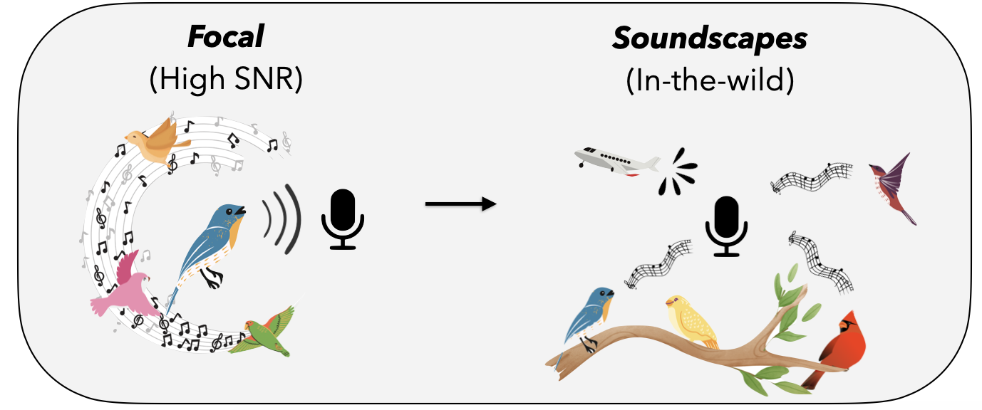
Naturally-occurring distribution shifts are ubiquitous in bioacoustics. The largest labeled dataset for bird songs is Xeno-Canto (XC), a collection of user-contributed recordings of wild birds from across the world. Recordings in XC are “focal”: they target an individual captured in natural conditions, where the song of the identified bird is at the foreground. For continuous monitoring and tracking purposes, though, practitioners are often more interested in identifying birds in passive recordings (“soundscapes”), obtained through omnidirectional microphones. This is a well-documented problem that recent work shows is very challenging. Inspired by this realistic application, we study SFDA in bioacoustics using a bird species classifier that was pre-trained on XC as the source model, and several “soundscapes” coming from different geographical locations — Sierra Nevada (S. Nevada); Powdermill Nature Reserve, Pennsylvania, USA; Hawai’i; Caples Watershed, California, USA; Sapsucker Woods, New York, USA (SSW); and Colombia — as our target domains.

This shift from the focalized to the passive domain is substantial: the recordings in the latter often feature much lower signal-to-noise ratio, several birds vocalizing at once, and significant distractors and environmental noise, like rain or wind. In addition, different soundscapes originate from different geographical locations, inducing extreme label shifts since a very small portion of the species in XC will appear in a given location. Moreover, as is common in real-world data, both the source and target domains are significantly class imbalanced, because some species are significantly more common than others. In addition, we consider a multi-label classification problem since there may be several birds identified within each recording, a significant departure from the standard single-label image classification scenario where SFDA is typically studied.

Illustration of the "focal → soundscapes" shift. In the focalized domain, recordings are typically composed of a single bird vocalization in the foreground, captured with high signal-to-noise ratio (SNR), though there may be other birds vocalizing in the background. On the other hand, soundscapes contain recordings from omnidirectional microphones and can be composed of multiple birds vocalizing simultaneously, as well as environmental noises from insects, rain, cars, planes, etc.

Audio files                 Focal domain
     
           Soundscape domain1
     
Spectogram images                 
Illustration of the distribution shift from the focal domain (left) to the soundscape domain (right), in terms of the audio files (top) and spectrogram images (bottom) of a representative recording from each dataset. Note that in the second audio clip, the bird song is very faint; a common property in soundscape recordings where bird calls aren’t at the “foreground”. Credits: Left: XC recording by Sue Riffe (CC-BY-NC license). Right: Excerpt from a recording made available by Kahl, Charif, & Klinck. (2022) "A collection of fully-annotated soundscape recordings from the Northeastern United States" [link] from the SSW soundscape dataset (CC-BY license).

State-of-the-art SFDA models perform poorly on bioacoustics shifts

As a starting point, we benchmark six state-of-the-art SFDA methods on our bioacoustics benchmark, and compare them to the non-adapted baseline (the source model). Our findings are surprising: without exception, existing methods are unable to consistently outperform the source model on all target domains. In fact, they often underperform it significantly.

As an example, Tent, a recent method, aims to make models produce confident predictions for each example by reducing the uncertainty of the model's output probabilities. While Tent performs well in various tasks, it doesn't work effectively for our bioacoustics task. In the single-label scenario, minimizing entropy forces the model to choose a single class for each example confidently. However, in our multi-label scenario, there's no such constraint that any class should be selected as being present. Combined with significant distribution shifts, this can cause the model to collapse, leading to zero probabilities for all classes. Other benchmarked methods like SHOT, AdaBN, Tent, NRC, DUST and Pseudo-Labelling, which are strong baselines for standard SFDA benchmarks, also struggle with this bioacoustics task.
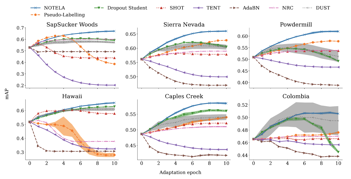
Evolution of the test mean average precision (mAP), a standard metric for multilabel classification, throughout the adaptation procedure on the six soundscape datasets. We benchmark our proposed NOTELA and Dropout Student (see below), as well as SHOT, AdaBN, Tent, NRC, DUST and Pseudo-Labelling. Aside from NOTELA, all other methods fail to consistently improve the source model.

Introducing NOisy student TEacher with Laplacian Adjustment (NOTELA)

Nonetheless, a surprisingly positive result stands out: the less celebrated Noisy Student principle appears promising. This unsupervised approach encourages the model to reconstruct its own predictions on some target dataset, but under the application of random noise. While noise may be introduced through various channels, we strive for simplicity and use model dropout as the only noise source: we therefore refer to this approach as Dropout Student (DS). In a nutshell, it encourages the model to limit the influence of individual neurons (or filters) when making predictions on a specific target dataset.

DS, while effective, faces a model collapse issue on various target domains. We hypothesize this happens because the source model initially lacks confidence in those target domains. We propose improving DS stability by using the feature space directly as an auxiliary source of truth. NOTELA does this by encouraging similar pseudo-labels for nearby points in the feature space, inspired by NRC's method and Laplacian regularization. This simple approach is visualized below, and consistently and significantly outperforms the source model in both audio and visual tasks.

NOTELA in action. The audio recordings are forwarded through the full model to obtain a first set of predictions, which are then refined through Laplacian regularization, a form of post-processing based on clustering nearby points. Finally, the refined predictions are used as targets for the noisy model to reconstruct.

Conclusion

The standard artificial image classification benchmarks have inadvertently limited our understanding of the true generalizability and robustness of SFDA methods. We advocate for broadening the scope and adopt a new assessment framework that incorporates naturally-occurring distribution shifts from bioacoustics. We also hope that NOTELA serves as a robust baseline to facilitate research in that direction. NOTELA’s strong performance perhaps points to two factors that can lead to developing more generalizable models: first, developing methods with an eye towards harder problems and second, favoring simple modeling principles. However, there is still future work to be done to pinpoint and comprehend existing methods’ failure modes on harder problems. We believe that our research represents a significant step in this direction, serving as a foundation for designing SFDA methods with greater generalizability.


Acknowledgements

One of the authors of this post, Eleni Triantafillou, is now at Google DeepMind. We are posting this blog post on behalf of the authors of the NOTELA paper: Malik Boudiaf, Tom Denton, Bart van Merriënboer, Vincent Dumoulin*, Eleni Triantafillou* (where * denotes equal contribution). We thank our co-authors for the hard work on this paper and the rest of the Perch team for their support and feedback.


1Note that in this audio clip, the bird song is very faint; a common property in soundscape recordings where bird calls aren’t at the “foreground”. 

Source: Google AI Blog


SoundStorm: Efficient parallel audio generation

The recent progress in generative AI unlocked the possibility of creating new content in several different domains, including text, vision and audio. These models often rely on the fact that raw data is first converted to a compressed format as a sequence of tokens. In the case of audio, neural audio codecs (e.g., SoundStream or EnCodec) can efficiently compress waveforms to a compact representation, which can be inverted to reconstruct an approximation of the original audio signal. Such a representation consists of a sequence of discrete audio tokens, capturing the local properties of sounds (e.g., phonemes) and their temporal structure (e.g., prosody). By representing audio as a sequence of discrete tokens, audio generation can be performed with Transformer-based sequence-to-sequence models — this has unlocked rapid progress in speech continuation (e.g., with AudioLM), text-to-speech (e.g., with SPEAR-TTS), and general audio and music generation (e.g., AudioGen and MusicLM). Many generative audio models, including AudioLM, rely on auto-regressive decoding, which produces tokens one by one. While this method achieves high acoustic quality, inference (i.e., calculating an output) can be slow, especially when decoding long sequences.

To address this issue, in “SoundStorm: Efficient Parallel Audio Generation”, we propose a new method for efficient and high-quality audio generation. SoundStorm addresses the problem of generating long audio token sequences by relying on two novel elements: 1) an architecture adapted to the specific nature of audio tokens as produced by the SoundStream neural codec, and 2) a decoding scheme inspired by MaskGIT, a recently proposed method for image generation, which is tailored to operate on audio tokens. Compared to the autoregressive decoding approach of AudioLM, SoundStorm is able to generate tokens in parallel, thus decreasing the inference time by 100x for long sequences, and produces audio of the same quality and with higher consistency in voice and acoustic conditions. Moreover, we show that SoundStorm, coupled with the text-to-semantic modeling stage of SPEAR-TTS, can synthesize high-quality, natural dialogues, allowing one to control the spoken content (via transcripts), speaker voices (via short voice prompts) and speaker turns (via transcript annotations), as demonstrated by the examples below:


Input: Text (transcript used to drive the audio generation in bold)        Something really funny happened to me this morning. | Oh wow, what? | Well, uh I woke up as usual. | Uhhuh | Went downstairs to have uh breakfast. | Yeah | Started eating. Then uh 10 minutes later I realized it was the middle of the night. | Oh no way, that's so funny!        I didn't sleep well last night. | Oh, no. What happened? | I don't know. I I just couldn't seem to uh to fall asleep somehow, I kept tossing and turning all night. | That's too bad. Maybe you should uh try going to bed earlier tonight or uh maybe you could try reading a book. | Yeah, thanks for the suggestions, I hope you're right. | No problem. I I hope you get a good night's sleep
         
Input: Audio prompt         
         
Output: Audio prompt + generated audio              


SoundStorm design

In our previous work on AudioLM, we showed that audio generation can be decomposed into two steps: 1) semantic modeling, which generates semantic tokens from either previous semantic tokens or a conditioning signal (e.g., a transcript as in SPEAR-TTS, or a text prompt as in MusicLM), and 2) acoustic modeling, which generates acoustic tokens from semantic tokens. With SoundStorm we specifically address this second, acoustic modeling step, replacing slower autoregressive decoding with faster parallel decoding.

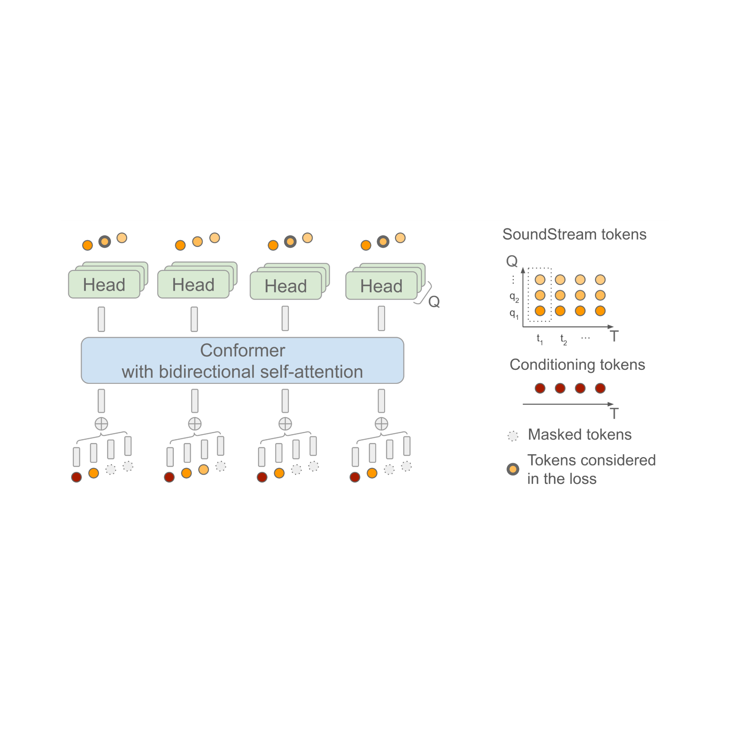
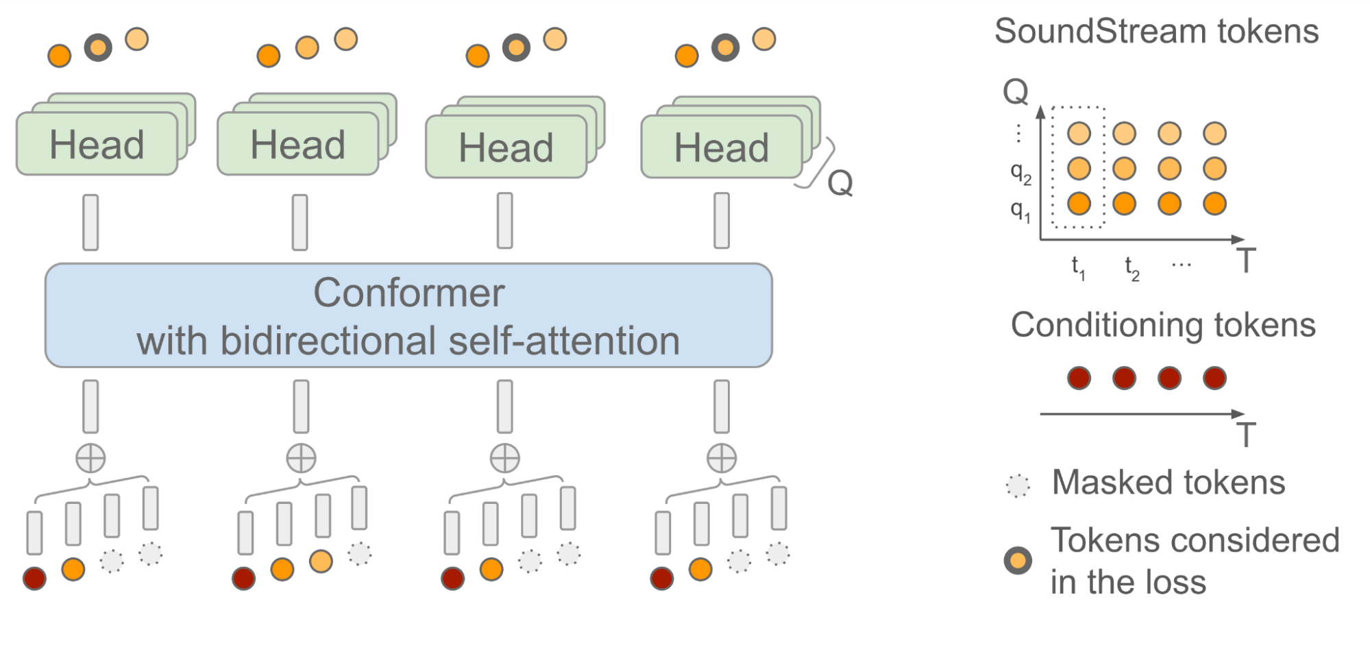
SoundStorm relies on a bidirectional attention-based Conformer, a model architecture that combines a Transformer with convolutions to capture both local and global structure of a sequence of tokens. Specifically, the model is trained to predict audio tokens produced by SoundStream given a sequence of semantic tokens generated by AudioLM as input. When doing this, it is important to take into account the fact that, at each time step t, SoundStream uses up to Q tokens to represent the audio using a method known as residual vector quantization (RVQ), as illustrated below on the right. The key intuition is that the quality of the reconstructed audio progressively increases as the number of generated tokens at each step goes from 1 to Q.

At inference time, given the semantic tokens as input conditioning signal, SoundStorm starts with all audio tokens masked out, and fills in the masked tokens over multiple iterations, starting from the coarse tokens at RVQ level q = 1 and proceeding level-by-level with finer tokens until reaching level q = Q.

There are two crucial aspects of SoundStorm that enable fast generation: 1) tokens are predicted in parallel during a single iteration within a RVQ level and, 2) the model architecture is designed in such a way that the complexity is only mildly affected by the number of levels Q. To support this inference scheme, during training a carefully designed masking scheme is used to mimic the iterative process used at inference.

SoundStorm model architecture. T denotes the number of time steps and Q the number of RVQ levels used by SoundStream. The semantic tokens used as conditioning are time-aligned with the SoundStream frames.

Measuring SoundStorm performance

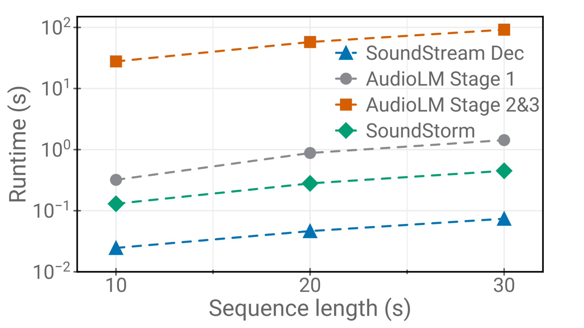
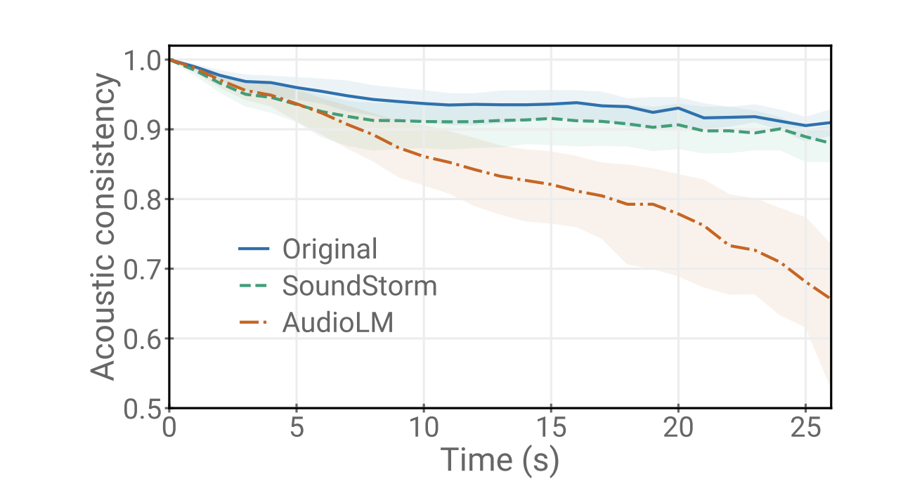
We demonstrate that SoundStorm matches the quality of AudioLM's acoustic generator, replacing both AudioLM's stage two (coarse acoustic model) and stage three (fine acoustic model). Furthermore, SoundStorm produces audio 100x faster than AudioLM's hierarchical autoregressive acoustic generator (top half below) with matching quality and improved consistency in terms of speaker identity and acoustic conditions (bottom half below).

Runtimes of SoundStream decoding, SoundStorm and different stages of AudioLM on a TPU-v4.
Acoustic consistency between the prompt and the generated audio. The shaded area represents the inter-quartile range.

Safety and risk mitigation

We acknowledge that the audio samples produced by the model may be influenced by the unfair biases present in the training data, for instance in terms of represented accents and voice characteristics. In our generated samples, we demonstrate that we can reliably and responsibly control speaker characteristics via prompting, with the goal of avoiding unfair biases. A thorough analysis of any training data and its limitations is an area of future work in line with our responsible AI Principles.

In turn, the ability to mimic a voice can have numerous malicious applications, including bypassing biometric identification and using the model for the purpose of impersonation. Thus, it is crucial to put in place safeguards against potential misuse: to this end, we have verified that the audio generated by SoundStorm remains detectable by a dedicated classifier using the same classifier as described in our original AudioLM paper. Hence, as a component of a larger system, we believe that SoundStorm would be unlikely to introduce additional risks to those discussed in our earlier papers on AudioLM and SPEAR-TTS. At the same time, relaxing the memory and computational requirements of AudioLM would make research in the domain of audio generation more accessible to a wider community. In the future, we plan to explore other approaches for detecting synthesized speech, e.g., with the help of audio watermarking, so that any potential product usage of this technology strictly follows our responsible AI Principles.


Conclusion

We have introduced SoundStorm, a model that can efficiently synthesize high-quality audio from discrete conditioning tokens. When compared to the acoustic generator of AudioLM, SoundStorm is two orders of magnitude faster and achieves higher temporal consistency when generating long audio samples. By combining a text-to-semantic token model similar to SPEAR-TTS with SoundStorm, we can scale text-to-speech synthesis to longer contexts and generate natural dialogues with multiple speaker turns, controlling both the voices of the speakers and the generated content. SoundStorm is not limited to generating speech. For example, MusicLM uses SoundStorm to synthesize longer outputs efficiently (as seen at I/O).


Acknowledgments

The work described here was authored by Zalán Borsos, Matt Sharifi, Damien Vincent, Eugene Kharitonov, Neil Zeghidour and Marco Tagliasacchi. We are grateful for all discussions and feedback on this work that we received from our colleagues at Google.

Source: Google AI Blog


The BirdCLEF 2023 Challenge: Pushing the frontiers of biodiversity monitoring

Worldwide bird populations are declining at an alarming rate, with approximately 48% of existing bird species known or suspected to be experiencing population declines. For instance, the U.S. and Canada have reported 29% fewer birds since 1970.

Effective monitoring of bird populations is essential for the development of solutions that promote conservation. Monitoring allows researchers to better understand the severity of the problem for specific bird populations and evaluate whether existing interventions are working. To scale monitoring, bird researchers have started analyzing ecosystems remotely using bird sound recordings instead of physically in-person via passive acoustic monitoring. Researchers can gather thousands of hours of audio with remote recording devices, and then use machine learning (ML) techniques to process the data. While this is an exciting development, existing ML models struggle with tropical ecosystem audio data due to higher bird species diversity and overlapping bird sounds.

Annotated audio data is needed to understand model quality in the real world. However, creating high-quality annotated datasets — especially for areas with high biodiversity — can be expensive and tedious, often requiring tens of hours of expert analyst time to annotate a single hour of audio. Furthermore, existing annotated datasets are rare and cover only a small geographic region, such as Sapsucker Woods or the Peruvian rainforest. Thousands of unique ecosystems in the world still need to be analyzed.

In an effort to tackle this problem, over the past 3 years, we've hosted ML competitions on Kaggle in partnership with specialized organizations focused on high-impact ecologies. In each competition, participants are challenged with building ML models that can take sounds from an ecology-specific dataset and accurately identify bird species by sound. The best entries can train reliable classifiers with limited training data. Last year’s competition focused on Hawaiian bird species, which are some of the most endangered in the world.


The 2023 BirdCLEF ML competition

This year we partnered with The Cornell Lab of Ornithology's K. Lisa Yang Center for Conservation Bioacoustics and NATURAL STATE to host the 2023 BirdCLEF ML competition focused on Kenyan birds. The total prize pool is $50,000, the entry deadline is May 17, 2023, and the final submission deadline is May 24, 2023. See the competition website for detailed information on the dataset to be used, timelines, and rules.

Kenya is home to over 1,000 species of birds, covering a wide range of ecosystems, from the savannahs of the Maasai Mara to the Kakamega rainforest, and even alpine regions on Kilimanjaro and Mount Kenya. Tracking this vast number of species with ML can be challenging, especially with minimal training data available for many species.

NATURAL STATE is working in pilot areas around Northern Mount Kenya to test the effect of various management regimes and states of degradation on bird biodiversity in rangeland systems. By using the ML algorithms developed within the scope of this competition, NATURAL STATE will be able to demonstrate the efficacy of this approach in measuring the success and cost-effectiveness of restoration projects. In addition, the ability to cost-effectively monitor the impact of restoration efforts on biodiversity will allow NATURAL STATE to test and build some of the first biodiversity-focused financial mechanisms to channel much-needed investment into the restoration and protection of this landscape upon which so many people depend. These tools are necessary to scale this cost-effectively beyond the project area and achieve their vision of restoring and protecting the planet at scale.

In previous competitions, we used metrics like the F1 score, which requires choosing specific detection thresholds for the models. This requires significant effort, and makes it difficult to assess the underlying model quality: A bad thresholding strategy on a good model may underperform. This year we are using a threshold-free model quality metric: class mean average precision. This metric treats each bird species output as a separate binary classifier to compute an average AUC score for each, and then averages these scores. Switching to an uncalibrated metric should increase the focus on core model quality by removing the need to choose a specific detection threshold.


How to get started

This will be the first Kaggle competition where participants can use the recently launched Kaggle Models platform that provides access to over 2,300 public, pre-trained models, including most of the TensorFlow Hub models. This new resource will have deep integrations with the rest of Kaggle, including Kaggle notebook, datasets, and competitions.

If you are interested in participating in this competition, a great place to get started quickly is to use our recently open-sourced Bird Vocalization Classifier model that is available on Kaggle Models. This global bird embedding and classification model provides output logits for more than 10k bird species and also creates embedding vectors that can be used for other tasks. Follow the steps shown in the figure below to use the Bird Vocalization Classifier model on Kaggle.

To try the model on Kaggle, navigate to the model here. 1) Click “New Notebook”; 2) click on the "Copy Code" button to copy the example lines of code needed to load the model; 3) click on the "Add Model" button to add this model as a data source to your notebook; and 4) paste the example code in the editor to load the model.

Alternatively, the competition starter notebook includes the model and extra code to more easily generate a competition submission.

We invite the research community to consider participating in the BirdCLEF competition. As a result of this effort, we hope that it will be easier for researchers and conservation practitioners to survey bird population trends and build effective conservation strategies.


Acknowledgements

Compiling these extensive datasets was a major undertaking, and we are very thankful to the many domain experts who helped to collect and manually annotate the data for this competition. Specifically, we would like to thank (institutions and individual contributors in alphabetic order): Julie Cattiau and Tom Denton on the Brain team, Maximilian Eibl and Stefan Kahl at Chemnitz University of Technology, Stefan Kahl and Holger Klinck from the K. Lisa Yang Center for Conservation Bioacoustics at the Cornell Lab of Ornithology, Alexis Joly and Henning Müller at LifeCLEF, Jonathan Baillie from NATURAL STATE, Hendrik Reers, Alain Jacot and Francis Cherutich from OekoFor GbR, and Willem-Pier Vellinga from xeno-canto. We would also like to thank Ian Davies from the Cornell Lab of Ornithology for allowing us to use the hero image in this post.

Source: Google AI Blog


AudioLM: a Language Modeling Approach to Audio Generation

Generating realistic audio requires modeling information represented at different scales. For example, just as music builds complex musical phrases from individual notes, speech combines temporally local structures, such as phonemes or syllables, into words and sentences. Creating well-structured and coherent audio sequences at all these scales is a challenge that has been addressed by coupling audio with transcriptions that can guide the generative process, be it text transcripts for speech synthesis or MIDI representations for piano. However, this approach breaks when trying to model untranscribed aspects of audio, such as speaker characteristics necessary to help people with speech impairments recover their voice, or stylistic components of a piano performance.

In “AudioLM: a Language Modeling Approach to Audio Generation”, we propose a new framework for audio generation that learns to generate realistic speech and piano music by listening to audio only. Audio generated by AudioLM demonstrates long-term consistency (e.g., syntax in speech, melody in music) and high fidelity, outperforming previous systems and pushing the frontiers of audio generation with applications in speech synthesis or computer-assisted music. Following our AI Principles, we've also developed a model to identify synthetic audio generated by AudioLM.

From Text to Audio Language Models
In recent years, language models trained on very large text corpora have demonstrated their exceptional generative abilities, from open-ended dialogue to machine translation or even common-sense reasoning. They have further shown their capacity to model other signals than texts, such as natural images. The key intuition behind AudioLM is to leverage such advances in language modeling to generate audio without being trained on annotated data.

However, some challenges need to be addressed when moving from text language models to audio language models. First, one must cope with the fact that the data rate for audio is significantly higher, thus leading to much longer sequences — while a written sentence can be represented by a few dozen characters, its audio waveform typically contains hundreds of thousands of values. Second, there is a one-to-many relationship between text and audio. This means that the same sentence can be rendered by different speakers with different speaking styles, emotional content and recording conditions.

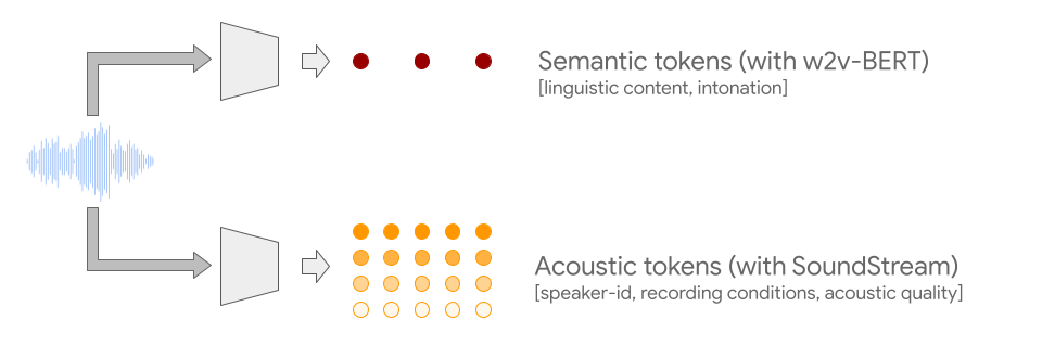
To overcome both challenges, AudioLM leverages two kinds of audio tokens. First, semantic tokens are extracted from w2v-BERT, a self-supervised audio model. These tokens capture both local dependencies (e.g., phonetics in speech, local melody in piano music) and global long-term structure (e.g., language syntax and semantic content in speech, harmony and rhythm in piano music), while heavily downsampling the audio signal to allow for modeling long sequences.

However, audio reconstructed from these tokens demonstrates poor fidelity. To overcome this limitation, in addition to semantic tokens, we rely on acoustic tokens produced by a SoundStream neural codec, which capture the details of the audio waveform (such as speaker characteristics or recording conditions) and allow for high-quality synthesis. Training a system to generate both semantic and acoustic tokens leads simultaneously to high audio quality and long-term consistency.

Training an Audio-Only Language Model
AudioLM is a pure audio model that is trained without any text or symbolic representation of music. AudioLM models an audio sequence hierarchically, from semantic tokens up to fine acoustic tokens, by chaining several Transformer models, one for each stage. Each stage is trained for the next token prediction based on past tokens, as one would train a text language model. The first stage performs this task on semantic tokens to model the high-level structure of the audio sequence.

In the second stage, we concatenate the entire semantic token sequence, along with the past coarse acoustic tokens, and feed both as conditioning to the coarse acoustic model, which then predicts the future tokens. This step models acoustic properties such as speaker characteristics in speech or timbre in music.

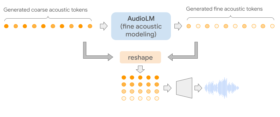
In the third stage, we process the coarse acoustic tokens with the fine acoustic model, which adds even more detail to the final audio. Finally, we feed acoustic tokens to the SoundStream decoder to reconstruct a waveform.

After training, one can condition AudioLM on a few seconds of audio, which enables it to generate consistent continuation. In order to showcase the general applicability of the AudioLM framework, we consider two tasks from different audio domains:

  • Speech continuation, where the model is expected to retain the speaker characteristics, prosody and recording conditions of the prompt while producing new content that is syntactically correct and semantically consistent.
  • Piano continuation, where the model is expected to generate piano music that is coherent with the prompt in terms of melody, harmony and rhythm.

In the video below, you can listen to examples where the model is asked to continue either speech or music and generate new content that was not seen during training. As you listen, note that everything you hear after the gray vertical line was generated by AudioLM and that the model has never seen any text or musical transcription, but rather just learned from raw audio. We release more samples on this webpage.

To validate our results, we asked human raters to listen to short audio clips and decide whether it is an original recording of human speech or a synthetic continuation generated by AudioLM. Based on the ratings collected, we observed a 51.2% success rate, which is not statistically significantly different from the 50% success rate achieved when assigning labels at random. This means that speech generated by AudioLM is hard to distinguish from real speech for the average listener.

Our work on AudioLM is for research purposes and we have no plans to release it more broadly at this time. In alignment with our AI Principles, we sought to understand and mitigate the possibility that people could misinterpret the short speech samples synthesized by AudioLM as real speech. For this purpose, we trained a classifier that can detect synthetic speech generated by AudioLM with very high accuracy (98.6%). This shows that despite being (almost) indistinguishable to some listeners, continuations generated by AudioLM are very easy to detect with a simple audio classifier. This is a crucial first step to help protect against the potential misuse of AudioLM, with future efforts potentially exploring technologies such as audio “watermarking”.

Conclusion
We introduce AudioLM, a language modeling approach to audio generation that provides both long-term coherence and high audio quality. Experiments on speech generation show not only that AudioLM can generate syntactically and semantically coherent speech without any text, but also that continuations produced by the model are almost indistinguishable from real speech by humans. Moreover, AudioLM goes well beyond speech and can model arbitrary audio signals such as piano music. This encourages the future extensions to other types of audio (e.g., multilingual speech, polyphonic music, and audio events) as well as integrating AudioLM into an encoder-decoder framework for conditioned tasks such as text-to-speech or speech-to-speech translation.

Acknowledgments
The work described here was authored by Zalán Borsos, Raphaël Marinier, Damien Vincent, Eugene Kharitonov, Olivier Pietquin, Matt Sharifi, Olivier Teboul, David Grangier, Marco Tagliasacchi and Neil Zeghidour. We are grateful for all discussions and feedback on this work that we received from our colleagues at Google.

Source: Google AI Blog


Separating Birdsong in the Wild for Classification

Birds are all around us, and just by listening, we can learn many things about our environment. Ecologists use birds to understand food systems and forest health — for example, if there are more woodpeckers in a forest, that means there’s a lot of dead wood. Because birds communicate and mark territory with songs and calls, it’s most efficient to identify them by ear. In fact, experts may identify up to 10x as many birds by ear as by sight.

In recent years, autonomous recording units (ARUs) have made it easy to capture thousands of hours of audio in forests that could be used to better understand ecosystems and identify critical habitat. However, manually reviewing the audio data is very time consuming, and experts in birdsong are rare. But an approach based on machine learning (ML) has the potential to greatly reduce the amount of expert review needed for understanding a habitat.

However, ML-based audio classification of bird species can be challenging for several reasons. For one, birds often sing over one another, especially during the “dawn chorus” when many birds are most active. Also, there aren’t clear recordings of individual birds to learn from — almost all of the available training data is recorded in noisy outdoor conditions, where other sounds from the wind, insects, and other environmental sources are often present. As a result, existing birdsong classification models struggle to identify quiet, distant and overlapping vocalizations. Additionally, some of the most common species often appear unlabeled in the background of training recordings for less common species, leading models to discount the common species. These difficult cases are very important for ecologists who want to identify endangered or invasive species using automated systems.

To address the general challenge of training ML models to automatically separate audio recordings without access to examples of isolated sounds, we recently proposed a new unsupervised method called mixture invariant training (MixIT) in our paper, “Unsupervised Sound Separation Using Mixture Invariant Training”. Moreover, in our new paper, “Improving Bird Classification with Unsupervised Sound Separation,” we use MixIT training to separate birdsong and improve species classification. We found that including the separated audio in the classification improves precision and classification quality on three independent soundscape datasets. We are also happy to announce the open-source release of the birdsong separation models on GitHub.

Bird Song Audio Separation
MixIT learns to separate single-channel recordings into multiple individual tracks, and can be trained entirely with noisy, real-world recordings. To train the separation model, we create a “mixture of mixtures” (MoM) by mixing together two real-world recordings. The separation model then learns to take the MoM apart into many channels to minimize a loss function that uses the two original real-world recordings as ground-truth references. The loss function uses these references to group the separated channels such that they can be mixed back together to recreate the two original real-world recordings. Since there’s no way to know how the different sounds in the MoM were grouped together in the original recordings, the separation model has no choice but to separate the individual sounds themselves, and thus learns to place each singing bird in a different output audio channel, also separate from wind and other background noise.

We trained a new MixIT separation model using birdsong recordings from Xeno-Canto and the Macaulay Library. We found that for separating birdsong, this new model outperformed a MixIT separation model trained on a large amount of general audio from the AudioSet dataset. We measure the quality of the separation by mixing two recordings together, applying separation, and then remixing the separated audio channels such that they reconstruct the original two recordings. We measure the signal-to-noise ratio (SNR) of the remixed audio relative to the original recordings. We found that the model trained specifically for birds achieved 6.1 decibels (dB) better SNR than the model trained on AudioSet (10.5 dB vs 4.4 dB). Subjectively, we also found many examples where the system worked incredibly well, separating very difficult to distinguish calls in real-world data.

The following videos demonstrate separation of birdsong from two different regions (Caples and the High Sierras). The videos show the mel-spectrogram of the mixed audio (a 2D image that shows the frequency content of the audio over time) and highlight the audio separated into different tracks.

High Sierras
  
Caples

Classifying Bird Species
To classify birds in real-world audio captured with ARUs, we first split the audio into five-second segments and then create a mel-spectrogram of each segment. We then train an EfficientNet classifier to identify bird species from the mel-spectrogram images, training on audio from Xeno-Canto and the Macaulay Library. We trained two separate classifiers, one for species in the Sierra Nevada mountains and one for upstate New York. Note that these classifiers are not trained on separated audio; that’s an area for future improvement.

We also introduced some new techniques to improve classifier training. Taxonomic training asks the classifier to provide labels for each level of the species taxonomy (genus, family, and order), which allows the model to learn groupings of species before learning the sometimes-subtle differences between similar species. Taxonomic training also allows the model to benefit from expert information about the taxonomic relationships between different species. We also found that random low-pass filtering was helpful for simulating distant sounds during training: As an audio source gets further away, the high-frequency parts fade away before the low-frequency parts. This was particularly effective for identifying species from the High Sierras region, where bird songs cover very long distances, unimpeded by trees.

Classifying Separated Audio
We found that separating audio with the new MixIT model before classification improved the classifier performance on three independent real-world datasets. The separation was particularly successful for identification of quiet and background birds, and in many cases helped with overlapping vocalizations as well.

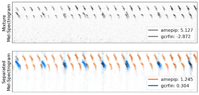
Top: A mel-spectrogram of two birds, an American pipit (amepip) and gray-crowned rosy finch (gcrfin), from the Sierra Nevadas. The legend shows the log-probabilities for the two species given by the pre-trained classifiers. Higher values indicate more confidence, and values greater than -1.0 are usually correct classifications. Bottom: A mel-spectrogram for the automatically separated audio, with the classifier log probabilities from the separated channels. Note that the classifier only identifies the gcrfin once the audio is separated.
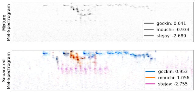
Top: A complex mixture with three vocalizations: A golden-crowned kinglet (gockin), mountain chickadee (mouchi), and Steller’s jay (stejay). Bottom: Separation into three channels, with classifier log probabilities for the three species. We see good visual separation of the Steller’s jay (shown by the distinct pink marks), even though the classifier isn’t sure what it is.

The separation model does have some potential limitations. Occasionally we observe over-separation, where a single song is broken into multiple channels, which can cause misclassifications. We also notice that when multiple birds are vocalizing, the most prominent song often gets a lower score after separation. This may be due to loss of environmental context or other artifacts introduced by separation that do not appear during classifier training. For now, we get the best results by running the classifier on the separated channels and the original audio, and taking the maximum score for each species. We expect that further work will allow us to reduce over-separation and find better ways to combine separation and classification. You can see and hear more examples of the full system at our GitHub repo.

Future Directions
We are currently working with partners at the California Academy of Sciences to understand how habitat and species mix changes after prescribed fires and wildfires, applying these models to ARU audio collected over many years.

We also foresee many potential applications for the unsupervised separation models in ecology, beyond just birds. For example, the separated audio can be used to create better acoustic indices, which could measure ecosystem health by tracking the total activity of birds, insects, and amphibians without identifying particular species. Similar methods could also be adapted for use underwater to track coral reef health.

Acknowledgements
We would like to thank Mary Clapp, Jack Dumbacher, and Durrell Kapan from the California Academy of Sciences for providing extensive annotated soundscapes from the Sierra Nevadas. Stefan Kahl and Holger Klinck from the Cornell Lab of Ornithology provided soundscapes from Sapsucker Woods. Training data for both the separation and classification models came from Xeno-Canto and the Macaulay Library. Finally, we would like to thank Julie Cattiau, Lauren Harrell, Matt Harvey, and our co-author, John Hershey, from the Google Bioacoustics and Sound Separation teams.

Source: Google AI Blog


LEAF: A Learnable Frontend for Audio Classification

Developing machine learning (ML) models for audio understanding has seen tremendous progress over the past several years. Leveraging the ability to learn parameters from data, the field has progressively shifted from composite, handcrafted systems to today’s deep neural classifiers that are used to recognize speech, understand music, or classify animal vocalizations such as bird calls. However, unlike computer vision models, which can learn from raw pixels, deep neural networks for audio classification are rarely trained from raw audio waveforms. Instead, they rely on pre-processed data in the form of mel filterbanks — handcrafted mel-scaled spectrograms that have been designed to replicate some aspects of the human auditory response.

Although modeling mel filterbanks for ML tasks has been historically successful, it is limited by the inherent biases of fixed features: even though using a fixed mel-scale and a logarithmic compression works well in general, we have no guarantee that they provide the best representations for the task at hand. In particular, even though matching human perception provides good inductive biases for some application domains, e.g., speech recognition or music understanding, these biases may be detrimental to domains for which imitating the human ear is not important, such as recognizing whale calls. So, in order to achieve optimal performance, the mel filterbanks should be tailored to the task of interest, a tedious process that requires an iterative effort informed by expert domain knowledge. As a consequence, standard mel filterbanks are used for most audio classification tasks in practice, even though they are suboptimal. In addition, while researchers have proposed ML systems to address these problems, such as Time-Domain Filterbanks, SincNet and Wavegram, they have yet to match the performance of traditional mel filterbanks.

In “LEAF, A Fully Learnable Frontend for Audio Classification”, accepted at ICLR 2021, we present an alternative method for crafting learnable spectrograms for audio understanding tasks. LEarnable Audio Frontend (LEAF) is a neural network that can be initialized to approximate mel filterbanks, and then be trained jointly with any audio classifier to adapt to the task at hand, while only adding a handful of parameters to the full model. We show that over a wide range of audio signals and classification tasks, including speech, music and bird songs, LEAF spectrograms improve classification performance over fixed mel filterbanks and over previously proposed learnable systems. We have implemented the code in TensorFlow 2 and released it to the community through our GitHub repository.

Mel Filterbanks: Mimicking Human Perception of Sound
The first step in the traditional approach to creating a mel filterbank is to capture the sound’s time-variability by windowing, i.e., cutting the signal into short segments with fixed duration. Then, one performs filtering, by passing the windowed segments through a bank of fixed frequency filters, that replicate the human logarithmic sensitivity to pitch. Because we are more sensitive to variations in low frequencies than high frequencies, mel filterbanks give more importance to the low-frequency range of sounds. Finally, the audio signal is compressed to mimic the ear’s logarithmic sensitivity to loudness — a sound needs to double its power for a person to perceive an increase of 3 decibels.

LEAF loosely follows this traditional approach to mel filterbank generation, but replaces each of the fixed operations (i.e., the filtering layer, windowing layer, and compression function) by a learned counterpart. The output of LEAF is a time-frequency representation (a spectrogram) similar to mel filterbanks, but fully learnable. So, for example, while a mel filterbank uses a fixed scale for pitch, LEAF learns the scale that is best suited to the task of interest. Any model that can be trained using mel filterbanks as input features, can also be trained on LEAF spectrograms.

Diagram of computation of mel filterbanks compared to LEAF spectrograms.

While LEAF can be initialized randomly, it can also be initialized in a way that approximates mel filterbanks, which have been shown to be a better starting point. Then, LEAF can be trained with any classifier to adapt to the task of interest.

Left: Mel filterbanks for a person saying “wow”. Right: LEAF’s output for the same example, after training on a dataset of speech commands.

A Parameter-Efficient Alternative to Fixed Features
A potential downside of replacing fixed features that involve no learnable parameter with a trainable system is that it can significantly increase the number of parameters to optimize. To avoid this issue, LEAF uses Gabor convolution layers that have only two parameters per filter, instead of the ~400 parameters typical of a standard convolution layer. This way, even when paired with a small classifier, such as EfficientNetB0, the LEAF model only accounts for 0.01% of the total parameters.

Top: Unconstrained convolutional filters after training for audio event classification. Bottom: LEAF filters at convergence after training for the same task.

Performance
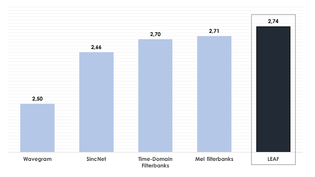
We apply LEAF to diverse audio classification tasks, including recognizing speech commands, speaker identification, acoustic scene recognition, identifying musical instruments, and finding birdsongs. On average, LEAF outperforms both mel filterbanks and previous learnable frontends, such as Time-Domain Filterbanks, SincNet and Wavegram. In particular, LEAF achieves a 76.9% average accuracy across the different tasks, compared to 73.9% for mel filterbanks. Moreover we show that LEAF can be trained in a multi-task setting, such that a single LEAF parametrization can work well across all these tasks. Finally, when combined with a large audio classifier, LEAF reaches state-of-the-art performance on the challenging AudioSet benchmark, with a 2.74 d-prime score.

D-prime score (the higher the better) of LEAF, mel filterbanks and previously proposed learnable spectrograms on the evaluation set of AudioSet.

Conclusion
The scope of audio understanding tasks keeps growing, from diagnosing dementia from speech to detecting humpback whale calls from underwater microphones. Adapting mel filterbanks to every new task can require a significant amount of hand-tuning and experimentation. In this context, LEAF provides a drop-in replacement for these fixed features, that can be trained to adapt to the task of interest, with minimal task-specific adjustments. Thus, we believe that LEAF can accelerate development of models for new audio understanding tasks.

Acknowledgements
We thank our co-authors, Olivier Teboul, Félix de Chaumont-Quitry and Marco Tagliasacchi. We also thank Dick Lyon, Vincent Lostanlen, Matt Harvey, and Alex Park for helpful discussions, and Julie Thomas for helping to design figures for this post.

Source: Google AI Blog


Improving End-to-End Models For Speech Recognition


Traditional automatic speech recognition (ASR) systems, used for a variety of voice search applications at Google, are comprised of an acoustic model (AM), a pronunciation model (PM) and a language model (LM), all of which are independently trained, and often manually designed, on different datasets [1]. AMs take acoustic features and predict a set of subword units, typically context-dependent or context-independent phonemes. Next, a hand-designed lexicon (the PM) maps a sequence of phonemes produced by the acoustic model to words. Finally, the LM assigns probabilities to word sequences. Training independent components creates added complexities and is suboptimal compared to training all components jointly. Over the last several years, there has been a growing popularity in developing end-to-end systems, which attempt to learn these separate components jointly as a single system. While these end-to-end models have shown promising results in the literature [2, 3], it is not yet clear if such approaches can improve on current state-of-the-art conventional systems.

Today we are excited to share “State-of-the-art Speech Recognition With Sequence-to-Sequence Models [4],” which describes a new end-to-end model that surpasses the performance of a conventional production system [1]. We show that our end-to-end system achieves a word error rate (WER) of 5.6%, which corresponds to a 16% relative improvement over a strong conventional system which achieves a 6.7% WER. Additionally, the end-to-end model used to output the initial word hypothesis, before any hypothesis rescoring, is 18 times smaller than the conventional model, as it contains no separate LM and PM.

Our system builds on the Listen-Attend-Spell (LAS) end-to-end architecture, first presented in [2]. The LAS architecture consists of 3 components. The listener encoder component, which is similar to a standard AM, takes the a time-frequency representation of the input speech signal, x, and uses a set of neural network layers to map the input to a higher-level feature representation, henc. The output of the encoder is passed to an attender, which uses henc to learn an alignment between input features x and predicted subword units {yn, … y0}, where each subword is typically a grapheme or wordpiece. Finally, the output of the attention module is passed to the speller (i.e., decoder), similar to an LM, that produces a probability distribution over a set of hypothesized words.
Components of the LAS End-to-End Model.
All components of the LAS model are trained jointly as a single end-to-end neural network, instead of as separate modules like conventional systems, making it much simpler.
Additionally, because the LAS model is fully neural, there is no need for external, manually designed components such as finite state transducers, a lexicon, or text normalization modules. Finally, unlike conventional models, training end-to-end models does not require bootstrapping from decision trees or time alignments generated from a separate system, and can be trained given pairs of text transcripts and the corresponding acoustics.

In [4], we introduce a variety of novel structural improvements, including improving the attention vectors passed to the decoder and training with longer subword units (i.e., wordpieces). In addition, we also introduce numerous optimization improvements for training, including the use of minimum word error rate training [5]. These structural and optimization improvements are what accounts for obtaining the 16% relative improvement over the conventional model.

Another exciting potential application for this research is multi-dialect and multi-lingual systems, where the simplicity of optimizing a single neural network makes such a model very attractive. Here data for all dialects/languages can be combined to train one network, without the need for a separate AM, PM and LM for each dialect/language. We find that these models work well on 7 english dialects [6] and 9 Indian languages [7], while outperforming a model trained separately on each individual language/dialect.

While we are excited by our results, our work is not done. Currently, these models cannot process speech in real time [8, 9], which is a strong requirement for latency-sensitive applications such as voice search. In addition, these models still compare negatively to production when evaluated on live production data. Furthermore, our end-to-end model is learned on 22,000 audio-text pair utterances compared to a conventional system that is typically trained on significantly larger corpora. In addition, our proposed model is not able to learn proper spellings for rarely used words such as proper nouns, which is normally performed with a hand-designed PM. Our ongoing efforts are focused now on addressing these challenges.

Acknowledgements
This work was done as a strong collaborative effort between Google Brain and Speech teams. Contributors include Tara Sainath, Rohit Prabhavalkar, Bo Li, Kanishka Rao, Shankar Kumar, Shubham Toshniwal, Michiel Bacchiani and Johan Schalkwyk from the Speech team; as well as Yonghui Wu, Patrick Nguyen, Zhifeng Chen, Chung-cheng Chiu, Anjuli Kannan, Ron Weiss and Navdeep Jaitly from the Google Brain team. The work is described in more detail in papers [4-11]

References
[1] G. Pundak and T. N. Sainath, “Lower Frame Rate Neural Network Acoustic Models," in Proc. Interspeech, 2016.

[2] W. Chan, N. Jaitly, Q. V. Le, and O. Vinyals, “Listen, attend and spell,” CoRR, vol. abs/1508.01211, 2015

[3] R. Prabhavalkar, K. Rao, T. N. Sainath, B. Li, L. Johnson, and N. Jaitly, “A Comparison of Sequence-to-sequence Models for Speech Recognition,” in Proc. Interspeech, 2017.

[4] C.C. Chiu, T.N. Sainath, Y. Wu, R. Prabhavalkar, P. Nguyen, Z. Chen, A. Kannan, R.J. Weiss, K. Rao, K. Gonina, N. Jaitly, B. Li, J. Chorowski and M. Bacchiani, “State-of-the-art Speech Recognition With Sequence-to-Sequence Models,” submitted to ICASSP 2018.

[5] R. Prabhavalkar, T.N. Sainath, Y. Wu, P. Nguyen, Z. Chen, C.C. Chiu and A. Kannan, “Minimum Word Error Rate Training for Attention-based Sequence-to-Sequence Models,” submitted to ICASSP 2018.

[6] B. Li, T.N. Sainath, K. Sim, M. Bacchiani, E. Weinstein, P. Nguyen, Z. Chen, Y. Wu and K. Rao, “Multi-Dialect Speech Recognition With a Single Sequence-to-Sequence Model” submitted to ICASSP 2018.

[7] S. Toshniwal, T.N. Sainath, R.J. Weiss, B. Li, P. Moreno, E. Weinstein and K. Rao, “End-to-End Multilingual Speech Recognition using Encoder-Decoder Models”, submitted to ICASSP 2018.

[8] T.N. Sainath, C.C. Chiu, R. Prabhavalkar, A. Kannan, Y. Wu, P. Nguyen and Z. Chen, “Improving the Performance of Online Neural Transducer Models”, submitted to ICASSP 2018.

[9] D. Lawson*, C.C. Chiu*, G. Tucker*, C. Raffel, K. Swersky, N. Jaitly. “Learning Hard Alignments with Variational Inference”, submitted to ICASSP 2018.

[10] T.N. Sainath, R. Prabhavalkar, S. Kumar, S. Lee, A. Kannan, D. Rybach, V. Schogol, P. Nguyen, B. Li, Y. Wu, Z. Chen and C.C. Chiu, “No Need for a Lexicon? Evaluating the Value of the Pronunciation Lexica in End-to-End Models,” submitted to ICASSP 2018.

[11] A. Kannan, Y. Wu, P. Nguyen, T.N. Sainath, Z. Chen and R. Prabhavalkar. “An Analysis of Incorporating an External Language Model into a Sequence-to-Sequence Model,” submitted to ICASSP 2018.