Tag Archives: Audio

LEAF: A Learnable Frontend for Audio Classification

Developing machine learning (ML) models for audio understanding has seen tremendous progress over the past several years. Leveraging the ability to learn parameters from data, the field has progressively shifted from composite, handcrafted systems to today’s deep neural classifiers that are used to recognize speech, understand music, or classify animal vocalizations such as bird calls. However, unlike computer vision models, which can learn from raw pixels, deep neural networks for audio classification are rarely trained from raw audio waveforms. Instead, they rely on pre-processed data in the form of mel filterbanks — handcrafted mel-scaled spectrograms that have been designed to replicate some aspects of the human auditory response.

Although modeling mel filterbanks for ML tasks has been historically successful, it is limited by the inherent biases of fixed features: even though using a fixed mel-scale and a logarithmic compression works well in general, we have no guarantee that they provide the best representations for the task at hand. In particular, even though matching human perception provides good inductive biases for some application domains, e.g., speech recognition or music understanding, these biases may be detrimental to domains for which imitating the human ear is not important, such as recognizing whale calls. So, in order to achieve optimal performance, the mel filterbanks should be tailored to the task of interest, a tedious process that requires an iterative effort informed by expert domain knowledge. As a consequence, standard mel filterbanks are used for most audio classification tasks in practice, even though they are suboptimal. In addition, while researchers have proposed ML systems to address these problems, such as Time-Domain Filterbanks, SincNet and Wavegram, they have yet to match the performance of traditional mel filterbanks.

In “LEAF, A Fully Learnable Frontend for Audio Classification”, accepted at ICLR 2021, we present an alternative method for crafting learnable spectrograms for audio understanding tasks. LEarnable Audio Frontend (LEAF) is a neural network that can be initialized to approximate mel filterbanks, and then be trained jointly with any audio classifier to adapt to the task at hand, while only adding a handful of parameters to the full model. We show that over a wide range of audio signals and classification tasks, including speech, music and bird songs, LEAF spectrograms improve classification performance over fixed mel filterbanks and over previously proposed learnable systems. We have implemented the code in TensorFlow 2 and released it to the community through our GitHub repository.

Mel Filterbanks: Mimicking Human Perception of Sound
The first step in the traditional approach to creating a mel filterbank is to capture the sound’s time-variability by windowing, i.e., cutting the signal into short segments with fixed duration. Then, one performs filtering, by passing the windowed segments through a bank of fixed frequency filters, that replicate the human logarithmic sensitivity to pitch. Because we are more sensitive to variations in low frequencies than high frequencies, mel filterbanks give more importance to the low-frequency range of sounds. Finally, the audio signal is compressed to mimic the ear’s logarithmic sensitivity to loudness — a sound needs to double its power for a person to perceive an increase of 3 decibels.

LEAF loosely follows this traditional approach to mel filterbank generation, but replaces each of the fixed operations (i.e., the filtering layer, windowing layer, and compression function) by a learned counterpart. The output of LEAF is a time-frequency representation (a spectrogram) similar to mel filterbanks, but fully learnable. So, for example, while a mel filterbank uses a fixed scale for pitch, LEAF learns the scale that is best suited to the task of interest. Any model that can be trained using mel filterbanks as input features, can also be trained on LEAF spectrograms.

Diagram of computation of mel filterbanks compared to LEAF spectrograms.

While LEAF can be initialized randomly, it can also be initialized in a way that approximates mel filterbanks, which have been shown to be a better starting point. Then, LEAF can be trained with any classifier to adapt to the task of interest.

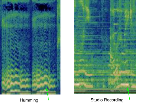
Left: Mel filterbanks for a person saying “wow”. Right: LEAF’s output for the same example, after training on a dataset of speech commands.

A Parameter-Efficient Alternative to Fixed Features
A potential downside of replacing fixed features that involve no learnable parameter with a trainable system is that it can significantly increase the number of parameters to optimize. To avoid this issue, LEAF uses Gabor convolution layers that have only two parameters per filter, instead of the ~400 parameters typical of a standard convolution layer. This way, even when paired with a small classifier, such as EfficientNetB0, the LEAF model only accounts for 0.01% of the total parameters.

Top: Unconstrained convolutional filters after training for audio event classification. Bottom: LEAF filters at convergence after training for the same task.

Performance
We apply LEAF to diverse audio classification tasks, including recognizing speech commands, speaker identification, acoustic scene recognition, identifying musical instruments, and finding birdsongs. On average, LEAF outperforms both mel filterbanks and previous learnable frontends, such as Time-Domain Filterbanks, SincNet and Wavegram. In particular, LEAF achieves a 76.9% average accuracy across the different tasks, compared to 73.9% for mel filterbanks. Moreover we show that LEAF can be trained in a multi-task setting, such that a single LEAF parametrization can work well across all these tasks. Finally, when combined with a large audio classifier, LEAF reaches state-of-the-art performance on the challenging AudioSet benchmark, with a 2.74 d-prime score.

D-prime score (the higher the better) of LEAF, mel filterbanks and previously proposed learnable spectrograms on the evaluation set of AudioSet.

Conclusion
The scope of audio understanding tasks keeps growing, from diagnosing dementia from speech to detecting humpback whale calls from underwater microphones. Adapting mel filterbanks to every new task can require a significant amount of hand-tuning and experimentation. In this context, LEAF provides a drop-in replacement for these fixed features, that can be trained to adapt to the task of interest, with minimal task-specific adjustments. Thus, we believe that LEAF can accelerate development of models for new audio understanding tasks.

Acknowledgements
We thank our co-authors, Olivier Teboul, Félix de Chaumont-Quitry and Marco Tagliasacchi. We also thank Dick Lyon, Vincent Lostanlen, Matt Harvey, and Alex Park for helpful discussions, and Julie Thomas for helping to design figures for this post.

Source: Google AI Blog


Lyra: A New Very Low-Bitrate Codec for Speech Compression

Connecting to others online via voice and video calls is something that is increasingly a part of everyday life. The real-time communication frameworks, like WebRTC, that make this possible depend on efficient compression techniques, codecs, to encode (or decode) signals for transmission or storage. A vital part of media applications for decades, codecs allow bandwidth-hungry applications to efficiently transmit data, and have led to an expectation of high-quality communication anywhere at any time.

As such, a continuing challenge in developing codecs, both for video and audio, is to provide increasing quality, using less data, and to minimize latency for real-time communication. Even though video might seem much more bandwidth hungry than audio, modern video codecs can reach lower bitrates than some high-quality speech codecs used today. Combining low-bitrate video and speech codecs can deliver a high-quality video call experience even in low-bandwidth networks. Yet historically, the lower the bitrate for an audio codec, the less intelligible and more robotic the voice signal becomes. Furthermore, while some people have access to a consistent high-quality, high-speed network, this level of connectivity isn’t universal, and even those in well connected areas at times experience poor quality, low bandwidth, and congested network connections.

To solve this problem, we have created Lyra, a high-quality, very low-bitrate speech codec that makes voice communication available even on the slowest networks. To do this, we’ve applied traditional codec techniques while leveraging advances in machine learning (ML) with models trained on thousands of hours of data to create a novel method for compressing and transmitting voice signals.

Lyra Overview
The basic architecture of the Lyra codec is quite simple. Features, or distinctive speech attributes, are extracted from speech every 40ms and are then compressed for transmission. The features themselves are log mel spectrograms, a list of numbers representing the speech energy in different frequency bands, which have traditionally been used for their perceptual relevance because they are modeled after human auditory response. On the other end, a generative model uses those features to recreate the speech signal. In this sense, Lyra is very similar to other traditional parametric codecs, such as MELP.

However traditional parametric codecs, which simply extract from speech critical parameters that can then be used to recreate the signal at the receiving end, achieve low bitrates, but often sound robotic and unnatural. These shortcomings have led to the development of a new generation of high-quality audio generative models that have revolutionized the field by being able to not only differentiate between signals, but also generate completely new ones. DeepMind’s WaveNet was the first of these generative models that paved the way for many to come. Additionally, WaveNetEQ, the generative model-based packet-loss-concealment system currently used in Duo, has demonstrated how this technology can be used in real-world scenarios.

A New Approach to Compression with Lyra
Using these models as a baseline, we’ve developed a new model capable of reconstructing speech using minimal amounts of data. Lyra harnesses the power of these new natural-sounding generative models to maintain the low bitrate of parametric codecs while achieving high quality, on par with state-of-the-art waveform codecs used in most streaming and communication platforms today. The drawback of waveform codecs is that they achieve this high quality by compressing and sending over the signal sample-by-sample, which requires a higher bitrate and, in most cases, isn’t necessary to achieve natural sounding speech.

One concern with generative models is their computational complexity. Lyra avoids this issue by using a cheaper recurrent generative model, a WaveRNN variation, that works at a lower rate, but generates in parallel multiple signals in different frequency ranges that it later combines into a single output signal at the desired sample rate. This trick enables Lyra to not only run on cloud servers, but also on-device on mid-range phones in real time (with a processing latency of 90ms, which is in line with other traditional speech codecs). This generative model is then trained on thousands of hours of speech data and optimized, similarly to WaveNet, to accurately recreate the input audio.

Comparison with Existing Codecs
Since the inception of Lyra, our mission has been to provide the best quality audio using a fraction of the bitrate data of alternatives. Currently, the royalty-free open-source codec Opus, is the most widely used codec for WebRTC-based VOIP applications and, with audio at 32kbps, typically obtains transparent speech quality, i.e., indistinguishable from the original. However, while Opus can be used in more bandwidth constrained environments down to 6kbps, it starts to demonstrate degraded audio quality. Other codecs are capable of operating at comparable bitrates to Lyra (Speex, MELP, AMR), but each suffer from increased artifacts and result in a robotic sounding voice.

Lyra is currently designed to operate at 3kbps and listening tests show that Lyra outperforms any other codec at that bitrate and is compared favorably to Opus at 8kbps, thus achieving more than a 60% reduction in bandwidth. Lyra can be used wherever the bandwidth conditions are insufficient for higher-bitrates and existing low-bitrate codecs do not provide adequate quality.

Clean Speech
Original
Opus@6kbps
Lyra@3kbps
Speex@3kbps
Noisy Environment
Original
Opus@6kbps
Lyra@3kbps
Speex@3kbps


ReferenceOpus@6kbpsLyra@3kbps


Ensuring Fairness
As with any ML based system, the model must be trained to make sure that it works for everyone. We’ve trained Lyra with thousands of hours of audio with speakers in over 70 languages using open-source audio libraries and then verifying the audio quality with expert and crowdsourced listeners. One of the design goals of Lyra is to ensure universally accessible high-quality audio experiences. Lyra trains on a wide dataset, including speakers in a myriad of languages, to make sure the codec is robust to any situation it might encounter.

Societal Impact and Where We Go From Here
The implications of technologies like Lyra are far reaching, both in the short and long term. With Lyra, billions of users in emerging markets can have access to an efficient low-bitrate codec that allows them to have higher quality audio than ever before. Additionally, Lyra can be used in cloud environments enabling users with various network and device capabilities to chat seamlessly with each other. Pairing Lyra with new video compression technologies, like AV1, will allow video chats to take place, even for users connecting to the internet via a 56kbps dial-in modem.

Duo already uses ML to reduce audio interruptions, and is currently rolling out Lyra to improve audio call quality and reliability on very low bandwidth connections. We will continue to optimize Lyra’s performance and quality to ensure maximum availability of the technology, with investigations into acceleration via GPUs and TPUs. We are also beginning to research how these technologies can lead to a low-bitrate general-purpose audio codec (i.e., music and other non-speech use cases).

Acknowledgements
Thanks to everyone who made Lyra possible including Jan Skoglund, Felicia Lim, Michael Chinen, Bastiaan Kleijn, Tom Denton, Andrew Storus, Yero Yeh (Chrome Media), Henrik Lundin, Niklas Blum, Karl Wiberg (Google Duo), Chenjie Gu, Zach Gleicher, Norman Casagrande, Erich Elsen (DeepMind).

Source: Google AI Blog


Navigating Recorder Transcripts Easily, with Smart Scrolling

Last year we launched Recorder, a new kind of recording app that made audio recording smarter and more useful by leveraging on-device machine learning (ML) to transcribe the recording, highlight audio events, and suggest appropriate tags for titles. Recorder makes editing, sharing and searching through transcripts easier. Yet because Recorder can transcribe very long recordings (up to 18 hours!), it can still be difficult for users to find specific sections, necessitating a new solution to quickly navigate such long transcripts.

To increase the navigability of content, we introduce Smart Scrolling, a new ML-based feature in Recorder that automatically marks important sections in the transcript, chooses the most representative keywords from each section, and then surfaces those keywords on the vertical scrollbar, like chapter headings. The user can then scroll through the keywords or tap on them to quickly navigate to the sections of interest. The models used are lightweight enough to be executed on-device without the need to upload the transcript, thus preserving user privacy.

Smart Scrolling feature UX

Under the hood
The Smart Scrolling feature is composed of two distinct tasks. The first extracts representative keywords from each section and the second picks which sections in the text are the most informative and unique.

For each task, we utilize two different natural language processing (NLP) approaches: a distilled bidirectional transformer (BERT) model pre-trained on data sourced from a Wikipedia dataset, alongside a modified extractive term frequency–inverse document frequency (TF-IDF) model. By using the bidirectional transformer and the TF-IDF-based models in parallel for both the keyword extraction and important section identification tasks, alongside aggregation heuristics, we were able to harness the advantages of each approach and mitigate their respective drawbacks (more on this in the next section).

The bidirectional transformer is a neural network architecture that employs a self-attention mechanism to achieve context-aware processing of the input text in a non-sequential fashion. This enables parallel processing of the input text to identify contextual clues both before and after a given position in the transcript.

Bidirectional Transformer-based model architecture

The extractive TF-IDF approach rates terms based on their frequency in the text compared to their inverse frequency in the trained dataset, and enables the finding of unique representative terms in the text.

Both models were trained on publicly available conversational datasets that were labeled and evaluated by independent raters. The conversational datasets were from the same domains as the expected product use cases, focusing on meetings, lectures, and interviews, thus ensuring the same word frequency distribution (Zipf’s law).

Extracting Representative Keywords
The TF-IDF-based model detects informative keywords by giving each word a score, which corresponds to how representative this keyword is within the text. The model does so, much like a standard TF-IDF model, by utilizing the ratio of the number of occurrences of a given word in the text compared to the whole of the conversational data set, but it also takes into account the specificity of the term, i.e., how broad or specific it is. Furthermore, the model then aggregates these features into a score using a pre-trained function curve. In parallel, the bidirectional transformer model, which was fine tuned on the task of extracting keywords, provides a deep semantic understanding of the text, enabling it to extract precise context-aware keywords.

The TF-IDF approach is conservative in the sense that it is prone to finding uncommon keywords in the text (high bias), while the drawback for the bidirectional transformer model is the high variance of the possible keywords that can be extracted. But when used together, these two models complement each other, forming a balanced bias-variance tradeoff.

Once the keyword scores are retrieved from both models, we normalize and combine them by utilizing NLP heuristics (e.g., the weighted average), removing duplicates across sections, and eliminating stop words and verbs. The output of this process is an ordered list of suggested keywords for each of the sections.

Rating A Section’s Importance
The next task is to determine which sections should be highlighted as informative and unique. To solve this task, we again combine the two models mentioned above, which yield two distinct importance scores for each of the sections. We compute the first score by taking the TF-IDF scores of all the keywords in the section and weighting them by their respective number of appearances in the section, followed by a summation of these individual keyword scores. We compute the second score by running the section text through the bidirectional transformer model, which was also trained on the sections rating task. The scores from both models are normalized and then combined to yield the section score.

Smart Scrolling pipeline architecture

Some Challenges
A significant challenge in the development of Smart Scrolling was how to identify whether a section or keyword is important - what is of great importance to one person can be of less importance to another. The key was to highlight sections only when it is possible to extract helpful keywords from them.

To do this, we configured the solution to select the top scored sections that also have highly rated keywords, with the number of sections highlighted proportional to the length of the recording. In the context of the Smart Scrolling features, a keyword was more highly rated if it better represented the unique information of the section.

To train the model to understand this criteria, we needed to prepare a labeled training dataset tailored to this task. In collaboration with a team of skilled raters, we applied this labeling objective to a small batch of examples to establish an initial dataset in order to evaluate the quality of the labels and instruct the raters in cases where there were deviations from what was intended. Once the labeling process was complete we reviewed the labeled data manually and made corrections to the labels as necessary to align them with our definition of importance.

Using this limited labeled dataset, we ran automated model evaluations to establish initial metrics on model quality, which were used as a less-accurate proxy to the model quality, enabling us to quickly assess the model performance and apply changes in the architecture and heuristics. Once the solution metrics were satisfactory, we utilized a more accurate manual evaluation process over a closed set of carefully chosen examples that represented expected Recorder use cases. Using these examples, we tweaked the model heuristics parameters to reach the desired level of performance using a reliable model quality evaluation.

Runtime Improvements
After the initial release of Recorder, we conducted a series of user studies to learn how to improve the usability and performance of the Smart Scrolling feature. We found that many users expect the navigational keywords and highlighted sections to be available as soon as the recording is finished. Because the computation pipeline described above can take a considerable amount of time to compute on long recordings, we devised a partial processing solution that amortizes this computation over the whole duration of the recording. During recording, each section is processed as soon as it is captured, and then the intermediate results are stored in memory. When the recording is done, Recorder aggregates the intermediate results.

When running on a Pixel 5, this approach reduced the average processing time of an hour long recording (~9K words) from 1 minute 40 seconds to only 9 seconds, while outputting the same results.

Summary
The goal of Recorder is to improve users’ ability to access their recorded content and navigate it with ease. We have already made substantial progress in this direction with the existing ML features that automatically suggest title words for recordings and enable users to search recordings for sounds and text. Smart Scrolling provides additional text navigation abilities that will further improve the utility of Recorder, enabling users to rapidly surface sections of interest, even for long recordings.

Acknowledgments
Bin Zhang, Sherry Lin, Isaac Blankensmith, Henry Liu‎, Vincent Peng‎, Guilherme Santos‎, Tiago Camolesi, Yitong Lin, James Lemieux, Thomas Hall‎, Kelly Tsai‎, Benny Schlesinger, Dror Ayalon, Amit Pitaru, Kelsie Van Deman, Console Chen, Allen Su, Cecile Basnage, Chorong Johnston‎, Shenaz Zack, Mike Tsao, Brian Chen, Abhinav Rastogi, Tracy Wu, Yvonne Yang‎.

Source: Google AI Blog


The Machine Learning Behind Hum to Search

Melodies stuck in your head, often referred to as “earworms,” are a well-known and sometimes irritating phenomenon — once that earworm is there, it can be tough to get rid of it. Research has found that engaging with the original song, whether that’s listening to or singing it, will drive the earworm away. But what if you can’t quite recall the name of the song, and can only hum the melody?

Existing methods to match a hummed melody to its original polyphonic studio recording face several challenges. With lyrics, background vocals and instruments, the audio of a musical or studio recording can be quite different from a hummed tune. By mistake or design, when someone hums their interpretation of a song, often the pitch, key, tempo or rhythm may vary slightly or even significantly. That’s why so many existing approaches to query by humming match the hummed tune against a database of pre-existing melody-only or hummed versions of a song, instead of identifying the song directly. However, this type of approach often relies on a limited database that requires manual updates.

Launched in October, Hum to Search is a new fully machine-learned system within Google Search that allows a person to find a song using only a hummed rendition of it. In contrast to existing methods, this approach produces an embedding of a melody from a spectrogram of a song without generating an intermediate representation. This enables the model to match a hummed melody directly to the original (polyphonic) recordings without the need for a hummed or MIDI version of each track or for other complex hand-engineered logic to extract the melody. This approach greatly simplifies the database for Hum to Search, allowing it to constantly be refreshed with embeddings of original recordings from across the world — even the latest releases.

Background
Many existing music recognition systems convert an audio sample into a spectrogram before processing it, in order to find a good match. However, one challenge in recognizing a hummed melody is that a hummed tune often contains relatively little information, as illustrated by this hummed example of Bella Ciao. The difference between the hummed version and the same segment from the corresponding studio recording can be visualized using spectrograms, seen below:

Visualization of a hummed clip and a matching studio recording.

Given the image on the left, a model needs to locate the audio corresponding to the right-hand image from a collection of over 50M similar-looking images (corresponding to segments of studio recordings of other songs). To achieve this, the model has to learn to focus on the dominant melody, and ignore background vocals, instruments, and voice timbre, as well as differences stemming from background noise or room reverberations. To find by eye the dominant melody that might be used to match these two spectrograms, a person might look for similarities in the lines near the bottom of the above images.

Prior efforts to enable discovery of music, in particular in the context of recognizing recorded music being played in an environment such as a cafe or a club, demonstrated how machine learning might be applied to this problem. Now Playing, released to Pixel phones in 2017, uses an on-device deep neural network to recognize songs without the need for a server connection, and Sound Search further developed this technology to provide a server-based recognition service for faster and more accurate searching of over 100 million songs. The next challenge then was to leverage what was learned from these releases to recognize hummed or sung music from a similarly large library of songs.

Machine Learning Setup
The first step in developing Hum to Search was to modify the music-recognition models used in Now Playing and Sound Search to work with hummed recordings. In principle, many such retrieval systems (e.g., image recognition) work in a similar way. A neural network is trained with pairs of input (here pairs of hummed or sung audio with recorded audio) to produce embeddings for each input, which will later be used for matching to a hummed melody.

Training setup for the neural network

To enable humming recognition, the network should produce embeddings for which pairs of audio containing the same melody are close to each other, even if they have different instrumental accompaniment and singing voices. Pairs of audio containing different melodies should be far apart. In training, the network is provided such pairs of audio until it learns to produce embeddings with this property.

The trained model can then generate an embedding for a tune that is similar to the embedding of the song’s reference recording. Finding the correct song is then only a matter of searching for similar embeddings from a database of reference recordings computed from audio of popular music.

Training Data
Because training of the model required song pairs (recorded and sung), the first challenge was to obtain enough training data. Our initial dataset consisted of mostly sung music segments (very few of these contained humming). To make the model more robust, we augmented the audio during training, for example by varying the pitch or tempo of the sung input randomly. The resulting model worked well enough for people singing, but not for people humming or whistling.

To improve the model’s performance on hummed melodies we generated additional training data of simulated “hummed” melodies from the existing audio dataset using SPICE, a pitch extraction model developed by our wider team as part of the FreddieMeter project. SPICE extracts the pitch values from given audio, which we then use to generate a melody consisting of discrete audio tones. The very first version of this system transformed this original clip into these tones.

Generating hummed audio from sung audio

We later refined this approach by replacing the simple tone generator with a neural network that generates audio resembling an actual hummed or whistled tune. For example, the network generates this humming example or whistling example from the above sung clip.

As a final step, we compared training data by mixing and matching the audio samples. For example, if we had a similar clip from two different singers, we’d align those two clips with our preliminary models, and are therefore able to show the model an additional pair of audio clips that represent the same melody.

Machine Learning Improvements
When training the Hum to Search model, we started with a triplet loss function. This loss has been shown to perform well across a variety of classification tasks like images and recorded music. Given a pair of audio corresponding to the same melody (points R and P in embedding space, shown below), triplet loss would ignore certain parts of the training data derived from a different melody. This helps the machine improve learning behavior, either when it finds a different melody that is too ‘easy’ in that it is already far away from R and P (see point E) or because it is too hard in that, given the model's current state of learning, the audio ends up being too close to R — even though according to our data it represents a different melody (see point H).

Example audio segments visualized as points in embedding space

We’ve found that we could improve the accuracy of the model by taking these additional training data (points H and E) into account, namely by formulating a general notion of model confidence across a batch of examples: How sure is the model that all the data it has seen can be classified correctly, or has it seen examples that do not fit its current understanding? Based on this notion of confidence, we added a loss that drives model confidence towards 100% across all areas of the embedding space, which led to improvements in our model’s precision and recall.

The above changes, but in particular our variations, augmentations and superpositions of the training data, enabled the neural network model deployed in Google Search to recognize sung or hummed melodies. The current system reaches a high level of accuracy on a song database that contains over half a million songs that we are continually updating. This song corpus still has room to grow to include more of the world’s many melodies.

Hum to Search in the Google App

To try the feature, you can open the latest version of the Google app, tap the mic icon and say “what's this song?” or click the “Search a song” button, after which you can hum, sing, or whistle away! We hope that Hum to Search can help with that earworm of yours, or maybe just help you in case you want to find and playback a song without having to type its name.

Acknowledgements
The work described here was authored by Alex Tudor, Duc Dung Nguyen, Matej Kastelic‎, Mihajlo Velimirović‎, Stefan Christoph, Mauricio Zuluaga, Christian Frank, Dominik Roblek, and Matt Sharifi. We would like to deeply thank Krishna Kumar, Satyajeet Salgar and Blaise Aguera y Arcas for their ongoing support, as well as all the Google teams we've collaborated with to build the full Hum to Search product.

We would also like to thank all our colleagues at Google who donated clips of themselves singing or humming and therefore laid a foundation for this work, as well as Nick Moukhine‎ for building the Google-internal singing donation app. Finally, special thanks to Meghan Danks and Krishna Kumar for their feedback on earlier versions of this post.

Source: Google AI Blog


Improving Audio Quality in Duo with WaveNetEQ


Online calls have become an everyday part of life for millions of people by helping to streamline their work and connect them to loved ones. To transmit a call across the internet, the data from calls are split into short chunks, called packets. These packets make their way over the network from the sender to the receiver where they are reassembled to make continuous streams of video and audio. However, packets often arrive at the other end in the wrong order or at the wrong time, an issue generally referred to as jitter, and sometimes individual packets can be lost entirely. Issues such as these lead to lower call quality, since the receiver has to try and fill in the gaps, and are a pervasive problem for both audio and video transmission. For example, 99% of Google Duo calls need to deal with packet losses, excessive jitter or network delays. Of those calls, 20% lose more than 3% of the total audio duration due to network issues, and 10% of calls lose more than 8%.
Simplified diagram of network problems leading to packet loss, which needs to be counteracted by the receiver to allow reliable real-time communication.
In order to ensure reliable real-time communication, it is necessary to deal with packets that are missing when the receiver needs them. Specifically, if new audio is not provided continuously, glitches and gaps will be audible, but repeating the same audio over and over is not an ideal solution, as it produces artifacts and reduces the overall quality of the call. The process of dealing with the missing packets is called packet loss concealment (PLC). The receiver’s PLC module is responsible for creating audio (or video) to fill in the gaps created by packet losses, excessive jitter or temporary network glitches, all three of which result in an absence of data.

To address these audio issues, we present WaveNetEQ, a new PLC system now being used in Duo. WaveNetEQ is a generative model, based on DeepMind’s WaveRNN technology, that is trained using a large corpus of speech data to realistically continue short speech segments enabling it to fully synthesize the raw waveform of missing speech. Because Duo calls are end-to-end encrypted, all processing needs to be done on-device. The WaveNetEQ model is fast enough to run on a phone, while still providing state-of-the-art audio quality and more natural sounding PLC than other systems currently in use.

A New PLC System for Duo
Like many other web-based communication systems, Duo is based on the WebRTC open source project. To conceal the effects of packet loss, WebRTC’s NetEQ component uses signal processing methods, which analyze the speech and produce a smooth continuation that works very well for small losses (20ms or less), but does not sound good when the number of missing packets leads to gaps of 60ms or more. In those latter cases the speech becomes robotic and repetitive, a characteristic sound that is unfortunately familiar to many internet voice callers.

To better manage packet loss, we replace the NetEQ PLC component with a modified version of WaveRNN, a recurrent neural network model for speech synthesis consisting of two parts, an autoregressive network and a conditioning network. The autoregressive network is responsible for the continuity of the signal and provides the short-term and mid-term structure for the speech by having each generated sample depend on the network’s previous outputs. The conditioning network influences the autoregressive network to produce audio that is consistent with the more slowly-moving input features.

However, WaveRNN, like its predecessor WaveNet, was created with the text-to-speech (TTS) application in mind. As a TTS model, WaveRNN is supplied with the information of what it is supposed to say and how to say it. The conditioning network directly receives this information as input in form of the phonemes that make up the words and additional prosody features (i.e., all non-text information like intonation or pitch). In a way, the conditioning network can “see into the future” and then steer the autoregressive network towards the right waveforms to match it. In the case of a PLC system and real-time communication, this context is not provided.

For a functional PLC system, one must both extract contextual information from the current speech (i.e., the past), and generate a plausible sound to continue it. Our solution, WaveNetEQ, does both at the same time, using the autoregressive network to provide the audio continuation during a packet loss event, and the conditioning network to model long term features, like voice characteristics. The spectrogram of the past audio signal is used as input for the conditioning network, which extracts limited information about the prosody and textual content. This condensed information is fed to the autoregressive network, which combines it with the audio of the recent past to predict the next sample in the waveform domain.

This differs slightly from the procedure that was followed during training of the WaveNetEQ model, where the autoregressive network receives the actual sample present in the training data as input for the next step, rather than using the last sample it produced. This process, called teacher forcing, assures that the model learns valuable information, even at an early stage of training when its predictions are still of low quality. Once the model is fully trained and put to use in an audio or video call, teacher forcing is only used to "warm up" the model for the first sample, and after that its own output is passed back as input for the next step.
WaveNetEQ architecture. During inference, we "warm up" the autoregressive network by teacher forcing with the most recent audio. Afterwards, the model is supplied with its own output as input for the next step. A MEL spectrogram from a longer audio part is used as input for the conditioning network.
The model is applied to the audio data in Duo's jitter buffer. Once the real audio continues after a packet loss event, we seamlessly merge the synthetic and real audio stream. In order to find the best alignment between the two signals, the model generates slightly more output than is required and then cross-fades from one to the other. This makes the transition smooth and avoids noticeable noise.
Simulation of PLC events on audio over a moving span of 60 ms. The blue line represents the real audio signal, including past and future parts of the PLC event. At each timestep the orange line represents the synthetic audio WaveNetEQ would predict if the audio were to cut out at the vertical grey line.
60 ms Packet Loss
NetEQ
WaveNetEQ
NetEQ
WaveNetEQ

120 ms Packet Loss
NetEQ
WaveNetEQ
NetEQ
WaveNetEQ
Audio clips: Comparison of WebRTC’s default PLC system, NetEQ, with our model, WaveNetEQ. Audio clips were taken from LibriTTS and 10% of the audio was dropped in 60 or 120 ms chunks and then filled in by the PLC systems.
Ensuring Robustness
One important factor during PLC is the ability of the network to adapt to variable input signals, including different speakers or changes in background noise. In order to ensure the robustness of the model across a wide range of users, we trained WaveNetEQ on a speech dataset that contains over 100 speakers in 48 different languages, which allows the model to learn the characteristics of human speech in general, instead of the properties of a specific language. To ensure WaveNetEQ is able to deal with noisy environments, such as answering your phone in the train station or in the cafeteria, we augment the data by mixing it with a wide variety of background noises.

While our model learns how to plausibly continue speech, this is only true on a short scale — it can finish a syllable but does not predict words, per se. Instead, for longer packet losses we gradually fade out until the model only produces silence after 120 milliseconds. To further ensure that the model is not generating false syllables, we evaluated samples from WaveNetEQ and NetEQ using the Google Cloud Speech-to-Text API and found no significant difference in the word error rate, i.e., how many mistakes were made transcribing the spoken text.

We have been experimenting with WaveNetEQ in Duo, where the feature has demonstrated a positive impact on call quality and user experience. WaveNetEQ is already available in all Duo calls on Pixel 4 phones and is now being rolled out to additional models.

Acknowledgements
The core team includes Alessio Bazzica, Niklas Blum, Lennart Kolmodin, Henrik Lundin, Alex Narest, Olga Sharonova from Google and Tom Walters from DeepMind. We would also like to thank Martin Bruse (Google), Norman Casagrande, Ray Smith, Chenjie Gu and Erich Elsen (DeepMind) for their contributions.

Source: Google AI Blog


The On-Device Machine Learning Behind Recorder


Over the past two decades, Google has made information widely accessible through search — from textual information, photos and videos, to maps and jobs. But much of the world’s information is conveyed through speech. Yet even though many people use audio recording devices to capture important information in conversations, interviews, lectures and more, it can be very difficult to later parse through hours of recordings to identify and extract information of interest. But what if there was the ability to automatically transcribe and tag long recordings in real-time, enabling you to intuitively find the relevant information you need, when you need it?

For this reason, we launched Recorder, a new kind of audio recording app for Pixel phones that leverages recent developments in on-device machine learning (ML) to transcribe conversations, to detect and identify the type of audio recorded (from broad categories like music or speech to particular sounds, such as applause, laughter and whistling), and to index recordings so users can quickly find and extract segments of interest. All of these features run entirely on-device, without the need for an internet connection.
Transcription
Recorder transcribes speech in real-time using an on-device automatic speech recognition model based on improvements announced earlier this year. Being a key component to many of Recorder’s smart features, we made sure that this model can transcribe long audio recordings (a few hours) reliably, while also indexing conversation by mapping words to timestamps as computed by the speech recognition model. This enables the user to click on a word in the transcription and initiate playback starting from that point in the recording, or to search for a word and jump to the exact point in the recording where it was being said.
Recording Content Visualization via Sound Classification
While presenting a transcript for a recording is useful and allows one to search for specific words, sometimes (especially for very long recordings) it’s more useful to visually search for sections of a recording based on specific moments or sounds. To enable this, Recorder additionally represents audio visually as a colored waveform where each color is associated with a different sound category. This is done by combining research into using CNNs to classify audio sounds (e.g., identifying a dog barking or a musical instrument playing) with previously published datasets for audio event detection to classify apparent sound events in individual audio frames.

Of course, in most situations many sounds can appear at the same time. In order to visualize the audio in a very clear way, we decided to color each waveform bar in a single color that represents the most dominant sound in a given time frame (in our case, 50ms bars). The colorized waveform lets users understand what type of content was captured in a specific recording and navigate along an ever-growing audio library more easily. This brings a visual representation of the audio recordings to the users, and also enables them to search over audio events in their recordings.
Recorder implements a sliding window capability that processes partially overlapping 960ms audio frames at 50ms intervals and outputs a sigmoid scores vector, representing the probability for each supported audio class within the frame. We apply a linearization process on the sigmoid scores in combination with a thresholding mechanism, in order to maximize the system precision and report the correct sound classification. This process of analyzing the content of the 960ms window with small 50ms offsets makes it possible to pinpoint exact start and end times in a manner that is less prone to mistakes than analyzing consecutive large 960ms window slices on their own.
Since the model analyzes each audio frame independently, it can be prone to quick jittering between audio classes. This is solved with an adaptive-size median filtering technique applied to the most recent model audio class outputs, thus providing a smoothed consecutive output. The process runs continuously in real-time, requiring it to meet very strict power consumption limitations.

Suggesting Tags for Titles
Once a recording is done, Recorder suggests three tags that the app deems to represent the most memorable content, enabling the user to quickly compose a meaningful title.
To be able to suggest these tags immediately when the recording ends, Recorder analyzes the content of the recording as it is being transcribed. First, Recorder counts term occurrences as well as their grammatical role in the sentence. The terms identified as entities are capitalized. Then, we utilize an on-device part-of-speech-tagger — a model that labels each word in the sentence according to its grammatical role — to detect common nouns and proper nouns, which appear to be more memorable by users. Recorder utilizes a prior scores table supporting both unigram and bigram terms extraction. To generate the scores, we trained a boosted decision tree with conversational data and utilized textual features like document words frequency and specificity. Last, filtering of stop words and swear words is applied and the top tags are outputted.
Tags extraction pipeline architecture
Conclusion
Recorder galvanized some of our most recent on-device ML research efforts into helpful features, running models on-device to ensure user privacy. The positive feedback loop between machine learning investigations and user needs revealed exciting opportunities to make our software even more useful. We’re excited for future research that will make everyone’s ideas and conversations even more easily accessible and searchable.

Acknowledgments
Special thanks to Dror Ayalon who played a key role in developing and forming the above features and without whom this blog post wouldn’t have been possible. We would also want to thank all our team members and collaborators who worked on this project with us: Amit Pitaru, Kelsie Van Deman, Isaac Blankensmith, Teo Soares, John Watkinson, Matt Hall, Josh Deitel, Benny Schlesinger, Yoni Tsafir, Michelle Tadmor Ramanovich, Danielle Cohen, Sushant Prakash, Renat Aksitov, Ed West, Max Gubin, Tiantian Zhang, Aaron Cohen, Yunhsuan Sung, Chung-Ching Chang, Nathan Dass, Amin Ahmad, Tiago Camolesi, Guilherme Santos‎, Julio da Silva, Dan Ellis, Qiao Liang, Arun Narayanan‎, Rohit Prabhavalkar, Benyah Shaparenko‎, Alex Salcianu, Mike Tsao, Shenaz Zak, Sherry Lin, James Lemieux, Jason Cho, Thomas Hall‎, Brian Chen, Allen Su, Vincent Peng‎, Richard Chou‎, Henry Liu‎, Edward Chen, Yitong Lin, Tracy Wu, Yvonne Yang‎.

Source: Google AI Blog


YouTube Music makes discovery more personal with playlists mixed for you

https://lh6.googleusercontent.com/vwz09fll1-AVy8mcSD49vSivK1h_eg__Nq97kubRgOW197eEQBm4_NfYt7sX7fDU98pltwhrN48Uk6Pt_i3aPM_ZeD9JlNjPGD8PSIKWOl7nt4n-L_aQa90XkCeGeyyvvh8fbRK0
YouTube Music is a dedicated music streaming service that guides you through the world of music. With official songs and albums as well as deep cuts, live performances, and remixes, you can listen to exactly what you want, when you want to. Or you can sit back and let us recommend music for you right on your home screen.


Rolling out today, we’re introducing a shelf of three personalized mixes -- the new Discover Mix, New Release Mix, and Your Mix -- to keep you up to date on what’s just been released and introduce you to a wider range of artists and sounds based on your personal taste. Updated regularly, these mixes will use your listening history to create a unique experience and guide your music exploration to exciting and fresh destinations week after week.


Check out what each of these new mixes is bringing to you:   


Discover Mix: Whether introducing you to an entirely new artist you’ve never heard before, or unearthing hidden, lesser-known gems from artists you’re already familiar with, Discover Mix will give you 50 tracks every week that help you expand your musical horizons. With new updates every Wednesday, it’s your go-to playlist to discover music. 


New Release Mix: This mix is your one-stop shop for a playlist of all the most recent releases by your favorite artists (and others we think you’ll like). Expect a big update every Friday (when most new releases drop) along with mid-week releases sprinkled in throughout the week to ensure you are always up-to-date on the latest releases. 


Your Mix: Your Mix is the perfect playlist for those times when you don’t want to think and just want to play something you know you’ll like. It’s full of songs by artists you know and love, and also mixes in some songs and artists you’ve never heard before, but that we think you’ll love. Small updates are made regularly, so the music never gets stale and there’s always something new in rotation. 


The more you listen to and like songs, the better your mixes will be. New to YouTube Music? Don’t worry, we can start delivering a personalized experience after you’ve selected a couple of artists you like during setup, or even after listening to just a few songs! 


Discover Mix, New Release Mix, and Your Mix are now available globally for all YouTube Music listeners. To check out your personalized mixes, download the YouTube Music app for iOS or Android or visit the webplayer to dive in.  


These new mixes are just the beginning of an even more personalized YouTube Music, so stay tuned for more music mixed just for you! 


Posted by Nathan Lasche, Product Manager, YouTube Music

Nathan recently listened to Dance Monkey by Tones and I

SPICE: Self-Supervised Pitch Estimation


A sound’s pitch is a qualitative measure of its frequency, where a sound with a high pitch is higher in frequency than one of low pitch. Through tracking relative differences in pitch, our auditory system is able to recognize audio features, such as a song’s melody. Pitch estimation has received a great deal of attention over the past decades, due to its central importance in several domains, ranging from music information retrieval to speech analysis.

Traditionally, simple signal processing pipelines were proposed to estimate pitch, working either in the time domain (e.g., pYIN) or in the frequency domain (e.g., SWIPE). But until recently, machine learning methods have not been able to outperform such hand-crafted signal processing pipelines. This was due to the lack of annotated data, which is particularly tedious and difficult to obtain at the temporal and frequency resolution required to train fully supervised models. The CREPE model was able to overcome these limitations to achieve state-of-the-art results by training on a synthetically generated dataset combined with other manually annotated datasets.

In our recent paper, we present a different approach to training pitch estimation models in the absence of annotated data. Inspired by the observation that for humans, including professional musicians, it is typically much easier to estimate relative pitch (the frequency interval between two notes) than absolute pitch (the true fundamental frequency), we designed SPICE (Self-supervised PItCh Estimation) to solve a similar task. This approach relies on self-supervision by defining an auxiliary task (also known as a pretext task) that can be learned in a completely unsupervised way.
Constant-Q transform of an audio clip, superimposed on a representation of pitch as estimated by SPICE (video).
The SPICE model consists of a convolutional encoder, which produces a single scalar embedding that maps linearly to pitch. To accomplish this, we feed two signals to the encoder, a reference signal along with a signal that is pitch shifted from the reference by a random, known amount. Then, we devise a loss function that forces the difference between the scalar embeddings to be proportional to the known difference in pitch. For convenience, we perform pitch shifting in the domain defined by the constant-Q transform (CQT), because this corresponds to a simple translation along the log-spaced frequency axis.

Pitch is well defined only when the underlying signal is harmonic, i.e., when it contains components with integer multiples of the fundamental frequency. So, an important function of the model is to determine when the output is meaningful and reliable. For example, in the figure below, there is no harmonic signal in the interval between 1.2s and 2s resulting in low enough confidence in the pitch estimation that no pitch estimate is generated. SPICE is designed to learn the level of confidence of the pitch estimation in a self-supervised fashion, instead of relying on handcrafted solutions.
SPICE model architecture (simplified). Two pitch-shifted versions of the same CQT frame are fed to two encoders with shared weights. The loss is designed to make the difference between the outputs of the encoders proportional to the relative pitch difference. In addition (not shown), a reconstruction loss is added to regularize the model. The model also learns to produce the confidence of the pitch estimation.
We evaluate our model against publicly available datasets and show that we outperform handcrafted baselines while matching the level of accuracy attained by CREPE, despite having no access to ground truth labels. In addition, by properly augmenting our data during training, SPICE is also able to operate in noisy conditions, e.g., to extract pitch from the singing voice when this is mixed in with background music. The chart below shows a comparison between SWIPE (a hand-crafted signal-processing method), CREPE (a fully supervised model) and SPICE (a self-supervised model) on the MIR-1k dataset.
Evaluation on the MIR-1k dataset, mixing in background music at different signal-to-noise ratios.
The SPICE model has been deployed in FreddieMeter, a web app in which singers can score their performance against Freddie Mercury.

Acknowledgments

The work described here was authored by Beat Gfeller, Christian Frank, Dominik Roblek, Matt Sharifi, Marco Tagliasacchi and Mihajlo Velimirović. We are grateful for all discussions and feedback on this work that we received from our colleagues at Google. The SingingVoices dataset used for training the models in this work has been collected by Alexandra Gherghina as part of FreddieMeter, which is using SPICE and a vocal timbre similarity model to understand how closely a singer matches Freddie Mercury.

Source: Google AI Blog


Audio and Visual Quality Measurement using Fréchet Distance


"I often say that when you can measure what you are speaking about, and express it in numbers, you know something about it; but when you cannot measure it, when you cannot express it in numbers, your knowledge is of a meagre and unsatisfactory kind.”
    William Thomson (Lord Kelvin), Lecture on "Electrical Units of Measurement" (3 May 1883), published in Popular Lectures Vol. I, p. 73
The rate of scientific progress in machine learning has often been determined by the availability of good datasets, and metrics. In deep learning, benchmark datasets such as ImageNet or Penn Treebank were among the driving forces that established deep artificial neural networks for image recognition and language modeling. Yet, while the available “ground-truth” datasets lend themselves nicely as measures of performance on these prediction tasks, determining the “ground-truth” for comparison to generative models is not so straightforward. Imagine a model that generates videos of StarCraft video game sequences — how does one determine which model is best? Clearly some of the videos shown below look more realistic than others, but can the differences between them be quantified? Access to robust metrics for evaluation of generative models is crucial for measuring (and making) progress in the fields of audio and video understanding, but currently no such metrics exist.
Videos generated from various models trained on sequences from the StarCraft Video (SCV) dataset.
In “Fréchet Audio Distance: A Metric for Evaluating Music Enhancement Algorithms” and “Towards Accurate Generative Models of Video: A New Metric & Challenges”, we present two such metrics — the Fréchet Audio Distance (FAD) and Fréchet Video Distance (FVD). We document our large-scale human evaluations using 10k video and 69k audio clip pairwise comparisons that demonstrate high correlations between our metrics and human perception. We are also releasing the source code for both Fréchet Video Distance and Fréchet Audio Distance on github (FVD; FAD).

General Description of Fréchet Distance
The goal of a generative model is to learn to produce samples that look similar to the ones on which it has been trained, such that it knows what properties and features are likely to appear in the data, and which ones are unlikely. In other words, a generative model must learn the probability distribution of the training data. In many cases, the target distributions for generative models are very high-dimensional. For example, a single image of 128x128 pixels with 3 color channels has almost 50k dimensions, while a second-long video clip might consist of dozens (or hundreds) of such frames with audio that may have 16,000 samples. Calculating distances between such high dimensional distributions in order to quantify how well a given model succeeds at a task is very difficult. In the case of pictures, one could look at a few samples to gauge visual quality, but doing so for every model trained is not feasible.

In addition, generative adversarial networks (GANs) tend to focus on a few modes of the overall target distribution, while completely ignoring others. For example, they may learn to generate only one type of object or only a select few viewing angles. As a consequence, looking only at a limited number of samples from the model may not indicate whether the network learned the entire distribution successfully. To remedy this, a metric is needed that aligns well with human judgement of quality, while also taking the properties of the target distribution into account.

One common solution for this problem is the so-called Fréchet Inception Distance (FID) metric, which was specifically designed for images. The FID takes a large number of images from both the target distribution and the generative model, and uses the Inception object-recognition network to embed each image into a lower-dimensional space that captures the important features. Then it computes the so-called Fréchet distance between these samples, which is a common way of calculating distances between distributions that provides a quantitative measure of how similar the two distributions actually are.
A key component for both metrics is a pre-trained model that converts the video or audio clip into an N-dimensional embedding.
Fréchet Audio Distance and Fréchet Video Distance
Building on the principles of FID that have been successfully applied to the image domain, we propose both Fréchet Video Distance (FVD) and Fréchet Audio Distance (FAD). Unlike popular metrics such as peak signal-to-noise ratio or the structural similarity index, FVD looks at videos in their entirety, and thereby avoids the drawbacks of framewise metrics.
Examples of videos of a robot arm, judged by the new FVD metric. FVD values were found to be approximately 2000, 1000, 600, 400, 300 and 150 (left-to-right; top-to-bottom). A lower FVD clearly correlates with higher video quality.
In the audio domain, existing metrics either require a time-aligned ground truth signal, such as source-to-distortion ratio (SDR), or only target a specific domain, like speech quality. FAD on the other hand is reference-free and can be used on any type of audio.

Below is a 2-D visualization of the audio embedding vectors from which we compute the FAD. Each point corresponds to the embedding of a 5-second audio clip, where the blue points are from clean music and other points represent audio that has been distorted in some way. The estimated multivariate Gaussian distributions are presented as concentric ellipses. As the magnitude of the distortions increase, the overlap between their distributions and that of the clean audio decreases. The separation between these distributions is what the Fréchet distance is measuring.
In the animation, we can see that as the magnitude of the distortions increases, the Gaussian distributions of the distorted audio overlaps less with the clean distribution. The magnitude of this separation is what the Fréchet distance is measuring.
Evaluation
It is important for FAD and FVD to closely track human judgement, since that is the gold standard for what looks and sounds “realistic”. So, we performed a large-scale human study to determine how well our new metrics align with qualitative human judgment of generated audio and video. For the study, human raters examined 10,000 video pairs and 69,000 5-second audio clips. For the FAD we asked human raters to compare the effect of two different distortions on the same audio segment, randomizing both the pair of distortions that they compared and the order in which they appeared. The raters were asked “Which audio clip sounds most like a studio-produced recording?” The collected set of pairwise evaluations was then ranked using a Plackett-Luce model, which estimates a worth value for each parameter configuration. Comparison of the worth values to the FAD demonstrates that the FAD correlates quite well with human judgement.
This figure compares the FAD calculated between clean background music and music distorted by a variety of methods (e.g., pitch down, Gaussian noise, etc.) to the associated worth values from human evaluation. Each type of distortion has two data points representing high and low extremes in the distortion applied. The quantization distortion (purple circles), for example, limits the audio to a specific number of bits per sample, where the two data points represent two different bitrates. Both human raters and the FAD assigned higher values (i.e., “less realistic”) to the lower bitrate quantization. Overall log FAD correlates well with human judgement — a perfect correlation between the log FAD and human perception would result in a straight line.
Conclusion
We are currently making great strides in generative models. FAD and FVD will help us keeping this progress measurable, and will hopefully lead us to improve our models for audio and video generation.

Acknowledgements
There are many people who contributed to this large effort, and we’d like to highlight some of the key contributors: Sjoerd van Steenkiste, Karol Kurach, Raphael Marinier, Marcin Michalski, Sylvain Gelly, Mauricio Zuluaga, Dominik Roblek, Matthew Sharifi as well as the extended Google Brain team in Zurich.

Source: Google AI Blog


What’s new with Fast Pair

Posted by Catherina Xu (Product Manager)

Last November, we released Fast Pair with the Jaybird Tarah Bluetooth headphones. Since then, we’ve engaged with dozens of OEMs, ODMs, and silicon partners to bring Fast Pair to even more devices. Last month, we held a talk at I/O announcing 10+ certified devices, support for Qualcomm’s Smart Headset Development Kit, and upcoming experiences for Fast Pair devices.

The Fast Pair team presenting at I/O 2019.

The Fast Pair team presenting at I/O 2019.

Upcoming experiences

Fast Pair makes pairing seamless across Android phones - this year, we are introducing additional features to improve Bluetooth device management.

  • True Wireless Features. As True Wireless Stereo (TWS) headphones continue to gain momentum in the market and with users, it is important to build system-wide support for TWS. Later this year, TWS headsets with Fast Pair will be able to broadcast individual battery information for the case and buds. This enables features such as case open and close battery notifications and per-component battery reporting throughout the UI.

     Detailed battery level notifications surfaced during “case open” for TWS headphones.

    Detailed battery level notifications surfaced during “case open” for TWS headphones.

    • Find My Device. Fast Pair devices will soon be surfaced in the Find My Device app and website, allowing users to easily track down lost devices. Headset owners can view the location and time of last use, as well as unpair or ring the buds to locate when they are in range.

    Connected Device Details. In Android Q, Fast Pair devices will have an enhanced Bluetooth device details page to centralize management and key settings. This includes links to Find My Device, Assistant settings (if available), and additional OEM-specified settings that will link to the OEM’s companion app.

    The updated Device details screen in Q allows easy access to key settings and the headphone’s companion app.

    The updated Device details screen in Q allows easy access to key settings and the headphone’s companion app.

    Compatible Devices

    Below is a list of devices that were showcased during our I/O talk:

    • Anker Spirit Pro GVA
    • Anker SoundCore Flare+ (Speaker)
    • JBL Live 220BT
    • JBL Live 400BT
    • JBL Live 500BT
    • JBL Live 650BT
    • Jaybird Tarah
    • 1More Dual Driver BT ANC
    • LG HBS-SL5
    • LG HBS-PL6S
    • LG HBS-SL6S
    • LG HBS-PL5
    • Cleer Ally Plus

    Interested in Fast Pair?

    If you are interested in creating Fast Pair compatible Bluetooth devices, please take a look at:

    Once you have selected devices to integrate, head to our Nearby Devices console to register your product. Reach out to us at [email protected] if you have any questions.