Author Archives: Andrew Helton

AMIE: A research AI system for diagnostic medical reasoning and conversations

The physician-patient conversation is a cornerstone of medicine, in which skilled and intentional communication drives diagnosis, management, empathy and trust. AI systems capable of such diagnostic dialogues could increase availability, accessibility, quality and consistency of care by being useful conversational partners to clinicians and patients alike. But approximating clinicians’ considerable expertise is a significant challenge.

Recent progress in large language models (LLMs) outside the medical domain has shown that they can plan, reason, and use relevant context to hold rich conversations. However, there are many aspects of good diagnostic dialogue that are unique to the medical domain. An effective clinician takes a complete “clinical history” and asks intelligent questions that help to derive a differential diagnosis. They wield considerable skill to foster an effective relationship, provide information clearly, make joint and informed decisions with the patient, respond empathically to their emotions, and support them in the next steps of care. While LLMs can accurately perform tasks such as medical summarization or answering medical questions, there has been little work specifically aimed towards developing these kinds of conversational diagnostic capabilities.

Inspired by this challenge, we developed Articulate Medical Intelligence Explorer (AMIE), a research AI system based on a LLM and optimized for diagnostic reasoning and conversations. We trained and evaluated AMIE along many dimensions that reflect quality in real-world clinical consultations from the perspective of both clinicians and patients. To scale AMIE across a multitude of disease conditions, specialties and scenarios, we developed a novel self-play based simulated diagnostic dialogue environment with automated feedback mechanisms to enrich and accelerate its learning process. We also introduced an inference time chain-of-reasoning strategy to improve AMIE’s diagnostic accuracy and conversation quality. Finally, we tested AMIE prospectively in real examples of multi-turn dialogue by simulating consultations with trained actors.

AMIE was optimized for diagnostic conversations, asking questions that help to reduce its uncertainty and improve diagnostic accuracy, while also balancing this with other requirements of effective clinical communication, such as empathy, fostering a relationship, and providing information clearly.

Evaluation of conversational diagnostic AI

Besides developing and optimizing AI systems themselves for diagnostic conversations, how to assess such systems is also an open question. Inspired by accepted tools used to measure consultation quality and clinical communication skills in real-world settings, we constructed a pilot evaluation rubric to assess diagnostic conversations along axes pertaining to history-taking, diagnostic accuracy, clinical management, clinical communication skills, relationship fostering and empathy.

We then designed a randomized, double-blind crossover study of text-based consultations with validated patient actors interacting either with board-certified primary care physicians (PCPs) or the AI system optimized for diagnostic dialogue. We set up our consultations in the style of an objective structured clinical examination (OSCE), a practical assessment commonly used in the real world to examine clinicians’ skills and competencies in a standardized and objective way. In a typical OSCE, clinicians might rotate through multiple stations, each simulating a real-life clinical scenario where they perform tasks such as conducting a consultation with a standardized patient actor (trained carefully to emulate a patient with a particular condition). Consultations were performed using a synchronous text-chat tool, mimicking the interface familiar to most consumers using LLMs today.

AMIE is a research AI system based on LLMs for diagnostic reasoning and dialogue.

AMIE: an LLM-based conversational diagnostic research AI system

We trained AMIE on real-world datasets comprising medical reasoning, medical summarization and real-world clinical conversations.

It is feasible to train LLMs using real-world dialogues developed by passively collecting and transcribing in-person clinical visits, however, two substantial challenges limit their effectiveness in training LLMs for medical conversations. First, existing real-world data often fails to capture the vast range of medical conditions and scenarios, hindering the scalability and comprehensiveness. Second, the data derived from real-world dialogue transcripts tends to be noisy, containing ambiguous language (including slang, jargon, humor and sarcasm), interruptions, ungrammatical utterances, and implicit references.

To address these limitations, we designed a self-play based simulated learning environment with automated feedback mechanisms for diagnostic medical dialogue in a virtual care setting, enabling us to scale AMIE’s knowledge and capabilities across many medical conditions and contexts. We used this environment to iteratively fine-tune AMIE with an evolving set of simulated dialogues in addition to the static corpus of real-world data described.

This process consisted of two self-play loops: (1) an “inner” self-play loop, where AMIE leveraged in-context critic feedback to refine its behavior on simulated conversations with an AI patient simulator; and (2) an “outer” self-play loop where the set of refined simulated dialogues were incorporated into subsequent fine-tuning iterations. The resulting new version of AMIE could then participate in the inner loop again, creating a virtuous continuous learning cycle.

Further, we also employed an inference time chain-of-reasoning strategy which enabled AMIE to progressively refine its response conditioned on the current conversation to arrive at an informed and grounded reply.

AMIE uses a novel self-play based simulated dialogue learning environment to improve the quality of diagnostic dialogue across a multitude of disease conditions, specialities and patient contexts.

We tested performance in consultations with simulated patients (played by trained actors), compared to those performed by 20 real PCPs using the randomized approach described above. AMIE and PCPs were assessed from the perspectives of both specialist attending physicians and our simulated patients in a randomized, blinded crossover study that included 149 case scenarios from OSCE providers in Canada, the UK and India in a diverse range of specialties and diseases.

Notably, our study was not designed to emulate either traditional in-person OSCE evaluations or the ways clinicians usually use text, email, chat or telemedicine. Instead, our experiment mirrored the most common way consumers interact with LLMs today, a potentially scalable and familiar mechanism for AI systems to engage in remote diagnostic dialogue.

Overview of the randomized study design to perform a virtual remote OSCE with simulated patients via online multi-turn synchronous text chat.

Performance of AMIE

In this setting, we observed that AMIE performed simulated diagnostic conversations at least as well as PCPs when both were evaluated along multiple clinically-meaningful axes of consultation quality. AMIE had greater diagnostic accuracy and superior performance for 28 of 32 axes from the perspective of specialist physicians, and 24 of 26 axes from the perspective of patient actors.
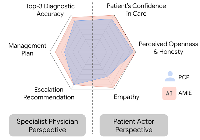
AMIE outperformed PCPs on multiple evaluation axes for diagnostic dialogue in our evaluations.
Specialist-rated top-k diagnostic accuracy. AMIE and PCPs top-k differential diagnosis (DDx) accuracy are compared across 149 scenarios with respect to the ground truth diagnosis (a) and all diagnoses listed within the accepted differential diagnoses (b). Bootstrapping (n=10,000) confirms all top-k differences between AMIE and PCP DDx accuracy are significant with p <0.05 after false discovery rate (FDR) correction.
Diagnostic conversation and reasoning qualities as assessed by specialist physicians. On 28 out of 32 axes, AMIE outperformed PCPs while being comparable on the rest.

Limitations

Our research has several limitations and should be interpreted with appropriate caution. Firstly, our evaluation technique likely underestimates the real-world value of human conversations, as the clinicians in our study were limited to an unfamiliar text-chat interface, which permits large-scale LLM–patient interactions but is not representative of usual clinical practice. Secondly, any research of this type must be seen as only a first exploratory step on a long journey. Transitioning from a LLM research prototype that we evaluated in this study to a safe and robust tool that could be used by people and those who provide care for them will require significant additional research. There are many important limitations to be addressed, including experimental performance under real-world constraints and dedicated exploration of such important topics as health equity and fairness, privacy, robustness, and many more, to ensure the safety and reliability of the technology.


AMIE as an aid to clinicians

In a recently released preprint, we evaluated the ability of an earlier iteration of the AMIE system to generate a DDx alone or as an aid to clinicians. Twenty (20) generalist clinicians evaluated 303 challenging, real-world medical cases sourced from the New England Journal of Medicine (NEJM) ClinicoPathologic Conferences (CPCs). Each case report was read by two clinicians randomized to one of two assistive conditions: either assistance from search engines and standard medical resources, or AMIE assistance in addition to these tools. All clinicians provided a baseline, unassisted DDx prior to using the respective assistive tools.

Assisted randomized reader study setup to investigate the assistive effect of AMIE to clinicians in solving complex diagnostic case challenges from the New England Journal of Medicine.

AMIE exhibited standalone performance that exceeded that of unassisted clinicians (top-10 accuracy 59.1% vs. 33.6%, p= 0.04). Comparing the two assisted study arms, the top-10 accuracy was higher for clinicians assisted by AMIE, compared to clinicians without AMIE assistance (24.6%, p<0.01) and clinicians with search (5.45%, p=0.02). Further, clinicians assisted by AMIE arrived at more comprehensive differential lists than those without AMIE assistance.

In addition to strong standalone performance, using the AMIE system led to significant assistive effect and improvements in diagnostic accuracy of the clinicians in solving these complex case challenges.

It's worth noting that NEJM CPCs are not representative of everyday clinical practice. They are unusual case reports in only a few hundred individuals so offer limited scope for probing important issues like equity or fairness.


Bold and responsible research in healthcare — the art of the possible

Access to clinical expertise remains scarce around the world. While AI has shown great promise in specific clinical applications, engagement in the dynamic, conversational diagnostic journeys of clinical practice requires many capabilities not yet demonstrated by AI systems. Doctors wield not only knowledge and skill but a dedication to myriad principles, including safety and quality, communication, partnership and teamwork, trust, and professionalism. Realizing these attributes in AI systems is an inspiring challenge that should be approached responsibly and with care. AMIE is our exploration of the “art of the possible”, a research-only system for safely exploring a vision of the future where AI systems might be better aligned with attributes of the skilled clinicians entrusted with our care. It is early experimental-only work, not a product, and has several limitations that we believe merit rigorous and extensive further scientific studies in order to envision a future in which conversational, empathic and diagnostic AI systems might become safe, helpful and accessible.


Acknowledgements

The research described here is joint work across many teams at Google Research and Google Deepmind. We are grateful to all our co-authors - Tao Tu, Mike Schaekermann, Anil Palepu, Daniel McDuff, Jake Sunshine, Khaled Saab, Jan Freyberg, Ryutaro Tanno, Amy Wang, Brenna Li, Mohamed Amin, Sara Mahdavi, Karan Sighal, Shekoofeh Azizi, Nenad Tomasev, Yun Liu, Yong Cheng, Le Hou, Albert Webson, Jake Garrison, Yash Sharma, Anupam Pathak, Sushant Prakash, Philip Mansfield, Shwetak Patel, Bradley Green, Ewa Dominowska, Renee Wong, Juraj Gottweis, Dale Webster, Katherine Chou, Christopher Semturs, Joelle Barral, Greg Corrado and Yossi Matias. We also thank Sami Lachgar, Lauren Winer and John Guilyard for their support with narratives and the visuals. Finally, we are grateful to Michael Howell, James Maynika, Jeff Dean, Karen DeSalvo, Zoubin Gharahmani and Demis Hassabis for their support during the course of this project.

Source: Google AI Blog


Differential Privacy Accounting by Connecting the Dots

Differential privacy (DP) is an approach that enables data analytics and machine learning (ML) with a mathematical guarantee on the privacy of user data. DP quantifies the “privacy cost” of an algorithm, i.e., the level of guarantee that the algorithm’s output distribution for a given dataset will not change significantly if a single user’s data is added to or removed from it. The algorithm is characterized by two parameters, ε and δ, where smaller values of both indicate “more private”. There is a natural tension between the privacy budget (ε, δ) and the utility of the algorithm: a smaller privacy budget requires the output to be more “noisy”, often leading to less utility. Thus, a fundamental goal of DP is to attain as much utility as possible for a desired privacy budget.

A key property of DP that often plays a central role in understanding privacy costs is that of composition, which reflects the net privacy cost of a combination of DP algorithms, viewed together as a single algorithm. A notable example is the differentially-private stochastic gradient descent (DP-SGD) algorithm. This algorithm trains ML models over multiple iterations — each of which is differentially private — and therefore requires an application of the composition property of DP. A basic composition theorem in DP says that the privacy cost of a collection of algorithms is, at most, the sum of the privacy cost of each. However, in many cases, this can be a gross overestimate, and several improved composition theorems provide better estimates of the privacy cost of composition.

In 2019, we released an open-source library (on GitHub) to enable developers to use analytic techniques based on DP. Today, we announce the addition to this library of Connect-the-Dots, a new privacy accounting algorithm based on a novel approach for discretizing privacy loss distributions that is a useful tool for understanding the privacy cost of composition. This algorithm is based on the paper “Connect the Dots: Tighter Discrete Approximations of Privacy Loss Distributions”, presented at PETS 2022. The main novelty of this accounting algorithm is that it uses an indirect approach to construct more accurate discretizations of privacy loss distributions. We find that Connect-the-Dots provides significant gains over other privacy accounting methods in literature in terms of accuracy and running time. This algorithm was also recently applied for the privacy accounting of DP-SGD in training Ads prediction models.


Differential Privacy and Privacy Loss Distributions

A randomized algorithm is said to satisfy DP guarantees if its output “does not depend significantly” on any one entry in its training dataset, quantified mathematically with parameters (ε, δ). For example, consider the motivating example of DP-SGD. When trained with (non-private) SGD, a neural network could, in principle, be encoding the entire training dataset within its weights, thereby allowing one to reconstruct some training examples from a trained model. On the other hand, when trained with DP-SGD, we have a formal guarantee that if one were able to reconstruct a training example with non-trivial probability then one would also be able to reconstruct the same example even if it was not included in the training dataset.

The hockey stick divergence, parameterized by ε, is a measure of distance between two probability distributions, as illustrated in the figure below. The privacy cost of most DP algorithms is dictated by the hockey stick divergence between two associated probability distributions P and Q. The algorithm satisfies DP with parameters (ε, δ), if the value of the hockey stick divergence for ε between P and Q is at most δ. The hockey stick divergence between (P, Q), denoted δP||Q(ε) is in turn completely characterized by it associated privacy loss distribution, denoted by PLDP||Q.

Illustration of hockey stick divergence δP||Q(ε) between distributions P and Q (left), which corresponds to the probability mass of P that is above eεQ, where eεQ is an eε scaling of the probability mass of Q (right).

The main advantage of dealing with PLDs is that compositions of algorithms correspond to the convolution of the corresponding PLDs. Exploiting this fact, prior work has designed efficient algorithms to compute the PLD corresponding to the composition of individual algorithms by simply performing convolution of the individual PLDs using the fast Fourier transform algorithm.

However, one challenge when dealing with many PLDs is that they often are continuous distributions, which make the convolution operations intractable in practice. Thus, researchers often apply various discretization approaches to approximate the PLDs using equally spaced points. For example, the basic version of the Privacy Buckets algorithm assigns the probability mass of the interval between two discretization points entirely to the higher end of the interval.

Illustration of discretization by rounding up probability masses. Here a continuous PLD (in blue) is discretized to a discrete PLD (in red), by rounding up the probability mass between consecutive points.

Connect-the-Dots : A New Algorithm

Our new Connect-the-Dots algorithm provides a better way to discretize PLDs towards the goal of estimating hockey stick divergences. This approach works indirectly by first discretizing the hockey stick divergence function and then mapping it back to a discrete PLD supported on equally spaced points.

Illustration of high-level steps in the Connect-the-Dots algorithm.

This approach relies on the notion of a “dominating PLD”, namely, PLDP’||Q’ dominates over PLDP||Q if the hockey stick divergence of the former is greater or equal to the hockey stick divergence of the latter for all values of ε. The key property of dominating PLDs is that they remain dominating after compositions. Thus for purposes of privacy accounting, it suffices to work with a dominating PLD, which gives us an upper bound on the exact privacy cost.

Our main insight behind the Connect-the-Dots algorithm is a characterization of discrete PLD, namely that a PLD is supported on a given finite set of ε values if and only if the corresponding hockey stick divergence as a function of eε is linear between consecutive eε values. This allows us to discretize the hockey stick divergence by simply connecting the dots to get a piecewise linear function that precisely equals the hockey stick divergence function at the given eε values. See a more detailed explanation of the algorithm.

Comparison of the discretizations of hockey stick divergence by Connect-the-Dots vs Privacy Buckets.

Experimental Evaluation

The DP-SGD algorithm involves a noise multiplier parameter, which controls the magnitude of noise added in each gradient step, and a sampling probability, which controls how many examples are included in each mini-batch. We compare Connect-the-Dots against the algorithms listed below on the task of privacy accounting DP-SGD with a noise multiplier = 0.5, sampling probability = 0.2 x 10⁻⁴ and δ = 10-8.

We plot the value of the ε computed by each of the algorithms against the number of composition steps, and additionally, we plot the running time of the implementations. As shown in the plots below, privacy accounting using Renyi DP provides a loose estimate of the privacy loss. However, when comparing the approaches using PLD, we find that in this example, the implementation of Connect-the-Dots achieves a tighter estimate of the privacy loss, with a running time that is 5x faster than the Microsoft PRV Accountant and >200x faster than the previous approach of Privacy Buckets in the Google-DP library.

Left: Upper bounds on the privacy parameter ε for varying number of steps of DP-SGD, as returned by different algorithms (for fixed δ = 10-8). Right: Running time of the different algorithms.

Conclusion & Future Directions

This work proposes Connect-the-Dots, a new algorithm for computing optimal privacy parameters for compositions of differentially private algorithms. When evaluated on the DP-SGD task, we find that this algorithm gives tighter estimates on the privacy loss with a significantly faster running time.

So far, the library only supports the pessimistic estimate version of Connect-the-Dots algorithm, which provides an upper bound on the privacy loss of DP-algorithms. However, the paper also introduces a variant of the algorithm that provides an “optimistic” estimate of the PLD, which can be used to derive lower bounds on the privacy cost of DP-algorithms (provided those admit a “worst case” PLD). Currently, the library does support optimistic estimates as given by the Privacy Buckets algorithm, and we hope to incorporate the Connect-the-Dots version as well.


Acknowledgements

This work was carried out in collaboration with Vadym Doroshenko, Badih Ghazi, Ravi Kumar. We thank Galen Andrew, Stan Bashtavenko, Steve Chien, Christoph Dibak, Miguel Guevara, Peter Kairouz, Sasha Kulankhina, Stefan Mellem, Jodi Spacek, Yurii Sushko and Andreas Terzis for their help.

Source: Google AI Blog


AudioLM: a Language Modeling Approach to Audio Generation

Generating realistic audio requires modeling information represented at different scales. For example, just as music builds complex musical phrases from individual notes, speech combines temporally local structures, such as phonemes or syllables, into words and sentences. Creating well-structured and coherent audio sequences at all these scales is a challenge that has been addressed by coupling audio with transcriptions that can guide the generative process, be it text transcripts for speech synthesis or MIDI representations for piano. However, this approach breaks when trying to model untranscribed aspects of audio, such as speaker characteristics necessary to help people with speech impairments recover their voice, or stylistic components of a piano performance.

In “AudioLM: a Language Modeling Approach to Audio Generation”, we propose a new framework for audio generation that learns to generate realistic speech and piano music by listening to audio only. Audio generated by AudioLM demonstrates long-term consistency (e.g., syntax in speech, melody in music) and high fidelity, outperforming previous systems and pushing the frontiers of audio generation with applications in speech synthesis or computer-assisted music. Following our AI Principles, we've also developed a model to identify synthetic audio generated by AudioLM.

From Text to Audio Language Models
In recent years, language models trained on very large text corpora have demonstrated their exceptional generative abilities, from open-ended dialogue to machine translation or even common-sense reasoning. They have further shown their capacity to model other signals than texts, such as natural images. The key intuition behind AudioLM is to leverage such advances in language modeling to generate audio without being trained on annotated data.

However, some challenges need to be addressed when moving from text language models to audio language models. First, one must cope with the fact that the data rate for audio is significantly higher, thus leading to much longer sequences — while a written sentence can be represented by a few dozen characters, its audio waveform typically contains hundreds of thousands of values. Second, there is a one-to-many relationship between text and audio. This means that the same sentence can be rendered by different speakers with different speaking styles, emotional content and recording conditions.

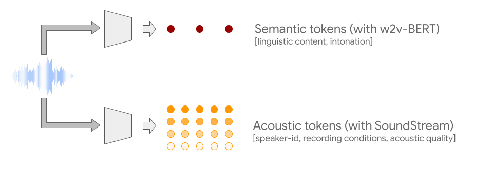
To overcome both challenges, AudioLM leverages two kinds of audio tokens. First, semantic tokens are extracted from w2v-BERT, a self-supervised audio model. These tokens capture both local dependencies (e.g., phonetics in speech, local melody in piano music) and global long-term structure (e.g., language syntax and semantic content in speech, harmony and rhythm in piano music), while heavily downsampling the audio signal to allow for modeling long sequences.

However, audio reconstructed from these tokens demonstrates poor fidelity. To overcome this limitation, in addition to semantic tokens, we rely on acoustic tokens produced by a SoundStream neural codec, which capture the details of the audio waveform (such as speaker characteristics or recording conditions) and allow for high-quality synthesis. Training a system to generate both semantic and acoustic tokens leads simultaneously to high audio quality and long-term consistency.

Training an Audio-Only Language Model
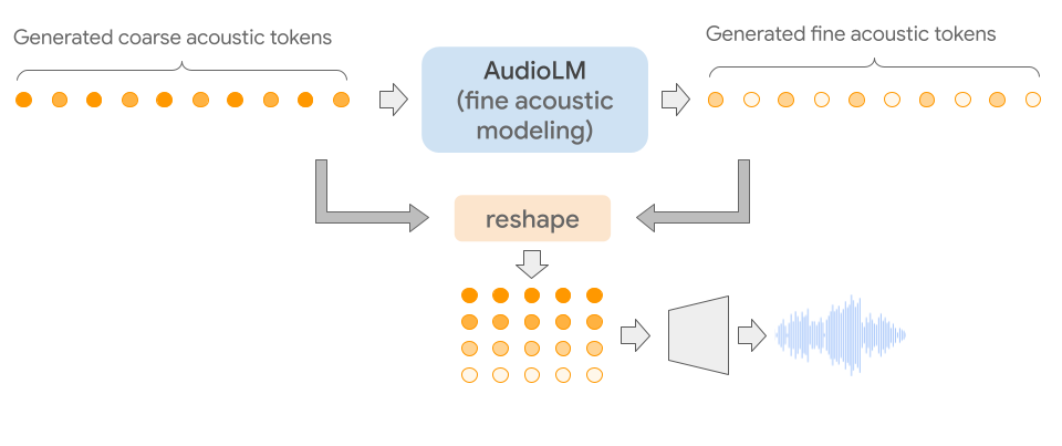
AudioLM is a pure audio model that is trained without any text or symbolic representation of music. AudioLM models an audio sequence hierarchically, from semantic tokens up to fine acoustic tokens, by chaining several Transformer models, one for each stage. Each stage is trained for the next token prediction based on past tokens, as one would train a text language model. The first stage performs this task on semantic tokens to model the high-level structure of the audio sequence.

In the second stage, we concatenate the entire semantic token sequence, along with the past coarse acoustic tokens, and feed both as conditioning to the coarse acoustic model, which then predicts the future tokens. This step models acoustic properties such as speaker characteristics in speech or timbre in music.

In the third stage, we process the coarse acoustic tokens with the fine acoustic model, which adds even more detail to the final audio. Finally, we feed acoustic tokens to the SoundStream decoder to reconstruct a waveform.

After training, one can condition AudioLM on a few seconds of audio, which enables it to generate consistent continuation. In order to showcase the general applicability of the AudioLM framework, we consider two tasks from different audio domains:

  • Speech continuation, where the model is expected to retain the speaker characteristics, prosody and recording conditions of the prompt while producing new content that is syntactically correct and semantically consistent.
  • Piano continuation, where the model is expected to generate piano music that is coherent with the prompt in terms of melody, harmony and rhythm.

In the video below, you can listen to examples where the model is asked to continue either speech or music and generate new content that was not seen during training. As you listen, note that everything you hear after the gray vertical line was generated by AudioLM and that the model has never seen any text or musical transcription, but rather just learned from raw audio. We release more samples on this webpage.

To validate our results, we asked human raters to listen to short audio clips and decide whether it is an original recording of human speech or a synthetic continuation generated by AudioLM. Based on the ratings collected, we observed a 51.2% success rate, which is not statistically significantly different from the 50% success rate achieved when assigning labels at random. This means that speech generated by AudioLM is hard to distinguish from real speech for the average listener.

Our work on AudioLM is for research purposes and we have no plans to release it more broadly at this time. In alignment with our AI Principles, we sought to understand and mitigate the possibility that people could misinterpret the short speech samples synthesized by AudioLM as real speech. For this purpose, we trained a classifier that can detect synthetic speech generated by AudioLM with very high accuracy (98.6%). This shows that despite being (almost) indistinguishable to some listeners, continuations generated by AudioLM are very easy to detect with a simple audio classifier. This is a crucial first step to help protect against the potential misuse of AudioLM, with future efforts potentially exploring technologies such as audio “watermarking”.

Conclusion
We introduce AudioLM, a language modeling approach to audio generation that provides both long-term coherence and high audio quality. Experiments on speech generation show not only that AudioLM can generate syntactically and semantically coherent speech without any text, but also that continuations produced by the model are almost indistinguishable from real speech by humans. Moreover, AudioLM goes well beyond speech and can model arbitrary audio signals such as piano music. This encourages the future extensions to other types of audio (e.g., multilingual speech, polyphonic music, and audio events) as well as integrating AudioLM into an encoder-decoder framework for conditioned tasks such as text-to-speech or speech-to-speech translation.

Acknowledgments
The work described here was authored by Zalán Borsos, Raphaël Marinier, Damien Vincent, Eugene Kharitonov, Olivier Pietquin, Matt Sharifi, Olivier Teboul, David Grangier, Marco Tagliasacchi and Neil Zeghidour. We are grateful for all discussions and feedback on this work that we received from our colleagues at Google.

Source: Google AI Blog


TensorStore for High-Performance, Scalable Array Storage

Many exciting contemporary applications of computer science and machine learning (ML) manipulate multidimensional datasets that span a single large coordinate system, for example, weather modeling from atmospheric measurements over a spatial grid or medical imaging predictions from multi-channel image intensity values in a 2d or 3d scan. In these settings, even a single dataset may require terabytes or petabytes of data storage. Such datasets are also challenging to work with as users may read and write data at irregular intervals and varying scales, and are often interested in performing analyses using numerous machines working in parallel.

Today we are introducing TensorStore, an open-source C++ and Python software library designed for storage and manipulation of n-dimensional data that:

TensorStore has already been used to solve key engineering challenges in scientific computing (e.g., management and processing of large datasets in neuroscience, such as peta-scale 3d electron microscopy data and “4d” videos of neuronal activity). TensorStore has also been used in the creation of large-scale machine learning models such as PaLM by addressing the problem of managing model parameters (checkpoints) during distributed training.

Familiar API for Data Access and Manipulation
TensorStore provides a simple Python API for loading and manipulating large array data. In the following example, we create a TensorStore object that represents a 56 trillion voxel 3d image of a fly brain and access a small 100x100 patch of the data as a NumPy array:

>>> import tensorstore as ts
>>> import numpy as np

# Create a TensorStore object to work with fly brain data.
>>> dataset = ts.open({
... 'driver':
... 'neuroglancer_precomputed',
... 'kvstore':
... 'gs://neuroglancer-janelia-flyem-hemibrain/v1.1/segmentation/',
... }).result()

# Create a 3-d view (remove singleton 'channel' dimension):
>>> dataset_3d = dataset[ts.d['channel'][0]]
>>> dataset_3d.domain
{ "x": [0, 34432), "y": [0, 39552), "z": [0, 41408) }

# Convert a 100x100x1 slice of the data to a numpy ndarray
>>> slice = np.array(dataset_3d[15000:15100, 15000:15100, 20000])

Crucially, no actual data is accessed or stored in memory until the specific 100x100 slice is requested; hence arbitrarily large underlying datasets can be loaded and manipulated without having to store the entire dataset in memory, using indexing and manipulation syntax largely identical to standard NumPy operations. TensorStore also provides extensive support for advanced indexing features, including transforms, alignment, broadcasting, and virtual views (data type conversion, downsampling, lazily on-the-fly generated arrays).

The following example demonstrates how TensorStore can be used to create a zarr array, and how its asynchronous API enables higher throughput:

>>> import tensorstore as ts
>>> import numpy as np

>>> # Create a zarr array on the local filesystem
>>> dataset = ts.open({
... 'driver': 'zarr',
... 'kvstore': 'file:///tmp/my_dataset/',
... },
... dtype=ts.uint32,
... chunk_layout=ts.ChunkLayout(chunk_shape=[256, 256, 1]),
... create=True,
... shape=[5000, 6000, 7000]).result()

>>> # Create two numpy arrays with example data to write.
>>> a = np.arange(100*200*300, dtype=np.uint32).reshape((100, 200, 300))
>>> b = np.arange(200*300*400, dtype=np.uint32).reshape((200, 300, 400))

>>> # Initiate two asynchronous writes, to be performed concurrently.
>>> future_a = dataset[1000:1100, 2000:2200, 3000:3300].write(a)
>>> future_b = dataset[3000:3200, 4000:4300, 5000:5400].write(b)

>>> # Wait for the asynchronous writes to complete
>>> future_a.result()
>>> future_b.result()

Safe and Performant Scaling
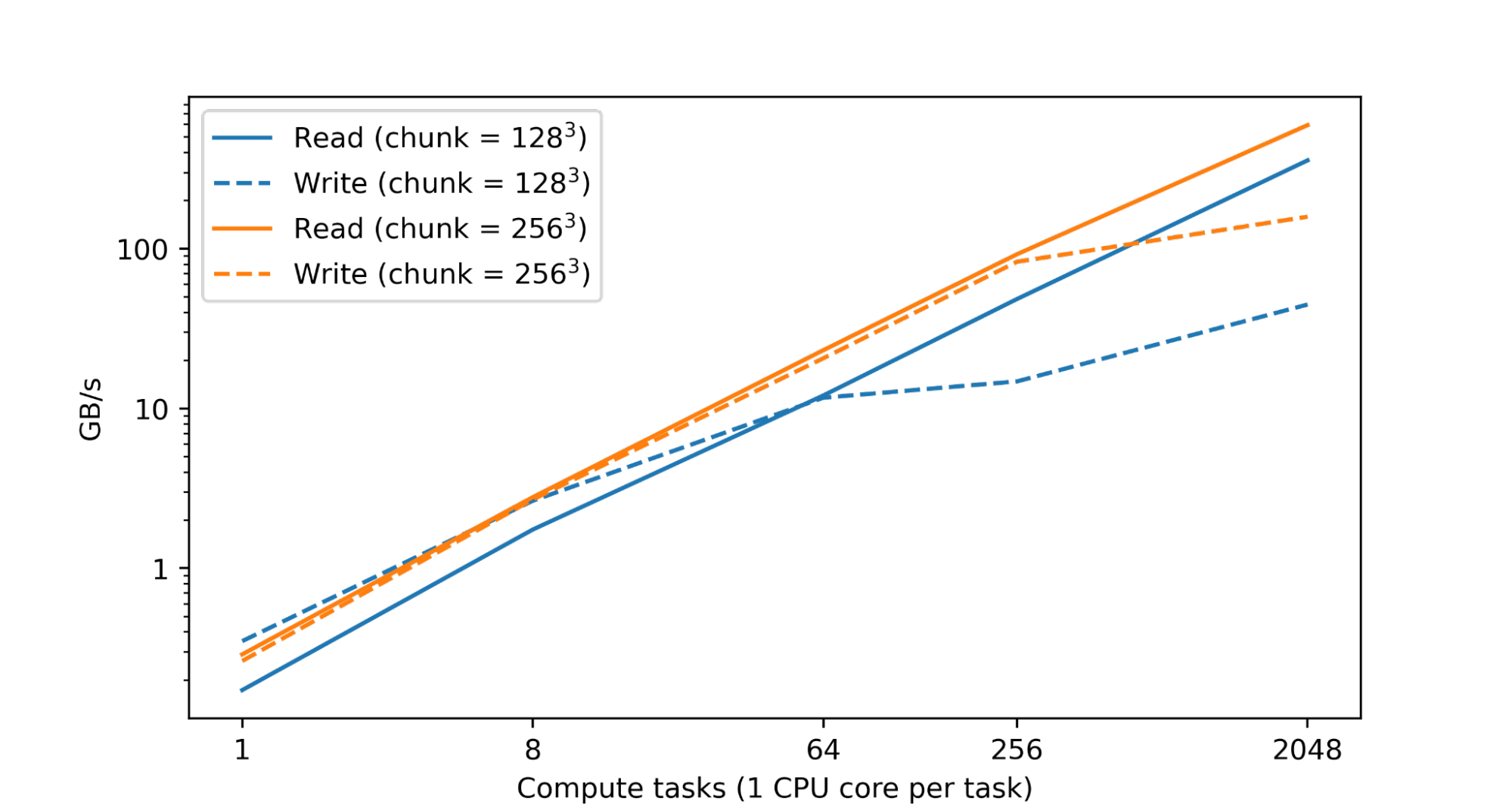
Processing and analyzing large numerical datasets requires significant computational resources. This is typically achieved through parallelization across numerous CPU or accelerator cores spread across many machines. Therefore a fundamental goal of TensorStore has been to enable parallel processing of individual datasets that is both safe (i.e., avoids corruption or inconsistencies arising from parallel access patterns) and high performance (i.e., reading and writing to TensorStore is not a bottleneck during computation). In fact, in a test within Google’s datacenters, we found nearly linear scaling of read and write performance as the number of CPUs was increased:

Read and write performance for a TensorStore dataset in zarr format residing on Google Cloud Storage (GCS) accessed concurrently using a variable number of single-core compute tasks in Google data centers. Both read and write performance scales nearly linearly with the number of compute tasks.

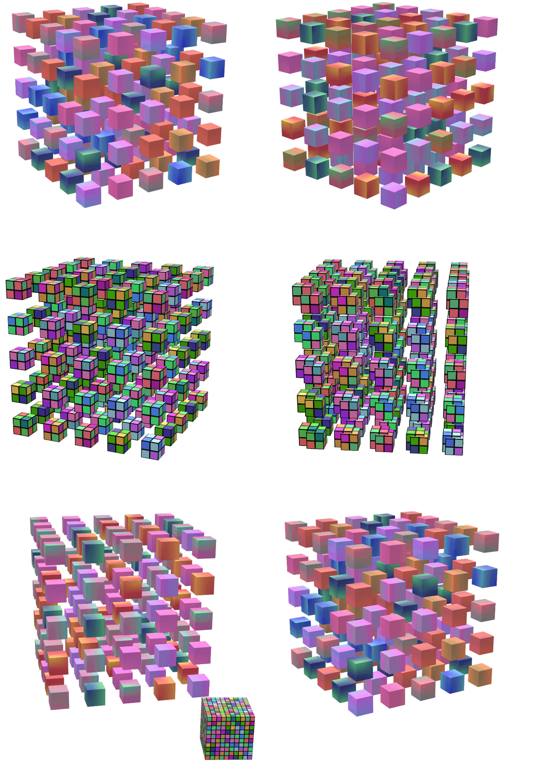
Performance is achieved by implementing core operations in C++, extensive use of multithreading for operations such as encoding/decoding and network I/O, and partitioning large datasets into much smaller units through chunking to enable efficiently reading and writing subsets of the entire dataset. TensorStore also provides configurable in-memory caching (which reduces slower storage system interactions for frequently accessed data) and an asynchronous API that enables a read or write operation to continue in the background while a program completes other work.

Safety of parallel operations when many machines are accessing the same dataset is achieved through the use of optimistic concurrency, which maintains compatibility with diverse underlying storage layers (including Cloud storage platforms, such as GCS, as well as local filesystems) without significantly impacting performance. TensorStore also provides strong ACID guarantees for all individual operations executing within a single runtime.

To make distributed computing with TensorStore compatible with many existing data processing workflows, we have also integrated TensorStore with parallel computing libraries such as Apache Beam (example code) and Dask (example code).

Use Case: Language Models
An exciting recent development in ML is the emergence of more advanced language models such as PaLM. These neural networks contain hundreds of billions of parameters and exhibit some surprising capabilities in natural language understanding and generation. These models also push the limits of computational infrastructure; in particular, training a language model such as PaLM requires thousands of TPUs working in parallel.

One challenge that arises during this training process is efficiently reading and writing the model parameters. Training is distributed across many separate machines, but parameters must be regularly saved to a single object (“checkpoint”) on a permanent storage system without slowing down the overall training process. Individual training jobs must also be able to read just the specific set of parameters they are concerned with in order to avoid the overhead that would be required to load the entire set of model parameters (which could be hundreds of gigabytes).

TensorStore has already been used to address these challenges. It has been applied to manage checkpoints associated with large-scale (“multipod”) models trained with JAX (code example) and has been integrated with frameworks such as T5X (code example) and Pathways. Model parallelism is used to partition the full set of parameters, which can occupy more than a terabyte of memory, over hundreds of TPUs. Checkpoints are stored in zarr format using TensorStore, with a chunk structure chosen to allow the partition for each TPU to be read and written independently in parallel.

When saving a checkpoint, each model parameter is written using TensorStore in zarr format using a chunk grid that further subdivides the grid used to partition the parameter over TPUs. The host machines write in parallel the zarr chunks for each of the partitions assigned to TPUs attached to that host. Using TensorStore's asynchronous API, training proceeds even while the data is still being written to persistent storage. When resuming from a checkpoint, each host reads only the chunks that make up the partitions assigned to that host.

Use Case: 3D Brain Mapping
The field of synapse-resolution connectomics aims to map the wiring of animal and human brains at the detailed level of individual synaptic connections. This requires imaging the brain at extremely high resolution (nanometers) over fields of view of up to millimeters or more, which yields datasets that can span petabytes in size. In the future these datasets may extend to exabytes as scientists contemplate mapping entire mouse or primate brains. However, even current datasets pose significant challenges related to storage, manipulation, and processing; in particular, even a single brain sample may require millions of gigabytes with a coordinate system (pixel space) of hundreds of thousands pixels in each dimension.

We have used TensorStore to solve computational challenges associated with large-scale connectomic datasets. Specifically, TensorStore has managed some of the largest and most widely accessed connectomic datasets, with Google Cloud Storage as the underlying object storage system. For example, it has been applied to the human cortex “h01” dataset, which is a 3d nanometer-resolution image of human brain tissue. The raw imaging data is 1.4 petabytes (roughly 500,000 * 350,000 * 5,000 pixels large, and is further associated with additional content such as 3d segmentations and annotations that reside in the same coordinate system. The raw data is subdivided into individual chunks 128x128x16 pixels large and stored in the “Neuroglancer precomputed” format, which is optimized for web-based interactive viewing and can be easily manipulated from TensorStore.

A fly brain reconstruction for which the underlying data can be easily accessed and manipulated using TensorStore.

Getting Started
To get started using the TensorStore Python API, you can install the tensorstore PyPI package using:

pip install tensorstore

Refer to the tutorials and API documentation for usage details. For other installation options and for using the C++ API, refer to installation instructions.

Acknowledgements
Thanks to Tim Blakely, Viren Jain, Yash Katariya, Jan-Matthis Luckmann, Michał Januszewski, Peter Li, Adam Roberts, Brain Williams, and Hector Yee from Google Research, and Davis Bennet, Stuart Berg, Eric Perlman, Stephen Plaza, and Juan Nunez-Iglesias from the broader scientific community for valuable feedback on the design, early testing and debugging.

Source: Google AI Blog


Identifying Disfluencies in Natural Speech

People don’t write in the same way that they speak. Written language is controlled and deliberate, whereas transcripts of spontaneous speech (like interviews) are hard to read because speech is disorganized and less fluent. One aspect that makes speech transcripts particularly difficult to read is disfluency, which includes self-corrections, repetitions, and filled pauses (e.g., words like “umm”, and “you know”). Following is an example of a spoken sentence with disfluencies from the LDC CALLHOME corpus:

But that's it's not, it's not, it's, uh, it's a word play on what you just said.

It takes some time to understand this sentence — the listener must filter out the extraneous words and resolve all of the nots. Removing the disfluencies makes the sentence much easier to read and understand:

But it’s a word play on what you just said.

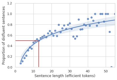
While people generally don't even notice disfluencies in day-to-day conversation, early foundational work in computational linguistics demonstrated how common they are. In 1994, using the Switchboard corpus, Elizabeh Shriberg demonstrated that there is a 50% probability for a sentence of 10–13 words to include a disfluency and that the probability increases with sentence length.

The proportion of sentences from the Switchboard dataset with at least one disfluency plotted against sentence length measured in non-disfluent (i.e., efficient) tokens in the sentence. The longer a sentence gets, the more likely it is to contain a disfluency.

In “Teaching BERT to Wait: Balancing Accuracy and Latency for Streaming Disfluency Detection”, we present research findings on how to “clean up” transcripts of spoken text. We create more readable transcripts and captions of human speech by finding and removing disfluencies in people’s speech. Using labeled data, we created machine learning (ML) algorithms that identify disfluencies in human speech. Once those are identified we can remove the extra words to make transcripts more readable. This also improves the performance of natural language processing (NLP) algorithms that work on transcripts of human speech. Our work puts special priority on ensuring that these models are able to run on mobile devices so that we can protect user privacy and preserve performance in scenarios with low connectivity.

Base Model Overview
At the core of our base model is a pre-trained BERTBASE encoder with 108.9 million parameters. We use the standard per-token classifier configuration, with a binary classification head being fed by the sequence encodings for each token.

Illustration of how tokens in text become numerical embeddings, which then lead to output labels.

We refined the BERT encoder by continuing the pretraining on the comments from the Pushrift Reddit dataset from 2019. Reddit comments are not speech data, but are more informal and conversational than the wiki and book data. This trains the encoder to better understand informal language, but may run the risk of internalizing some of the biases inherent in the data. For our particular use case, however, the model only captures the syntax or overall form of the text, not its content, which avoids potential issues related to semantic-level biases in the data.

We fine-tune our model for disfluency classification on hand-labeled corpora, such as the Switchboard corpus mentioned above. Hyperparameters (batch size, learning rate, number of training epochs, etc.) were optimized using Vizier.

We also produce a range of “small” models for use on mobile devices using a knowledge distillation technique known as “self training”. Our best small model is based on the Small-vocab BERT variant with 3.1 million parameters. This smaller model achieves comparable results to our baseline at 1% the size (in MiB). You can read more about how we achieved this model miniaturization in our 2021 Interspeech paper.

Streaming
Some of the latest use cases for automatic speech transcription include automated live captioning, such as produced by the Android “Live Captions” feature, which automatically transcribes spoken language in audio being played on the device. For disfluency removal to be of use in improving the readability of the captions in this setting, then it must happen quickly and in a stable manner. That is, the model should not change its past predictions as it sees new words in the transcript.

We call this live token-by-token processing streaming. Accurate streaming is difficult because of temporal dependencies; most disfluencies are only recognizable later. For example, a repetition does not actually become a repetition until the second time the word or phrase is said.

To investigate whether our disfluency detection model is effective in streaming applications, we split the utterances in our training set into prefix segments, where only the first N tokens of the utterance were provided at training time, for all values of N up to the full length of the utterance. We evaluated the model simulating a stream of spoken text by feeding prefixes to the models and measuring the performance with several metrics that capture model accuracy, stability, and latency including streaming F1, time to detection (TTD), edit overhead (EO), and average wait time (AWT). We experimented with look-ahead windows of either one or two tokens, allowing the model to “peek” ahead at additional tokens for which the model is not required to produce a prediction. In essence, we’re asking the model to “wait” for one or two more tokens of evidence before making a decision.

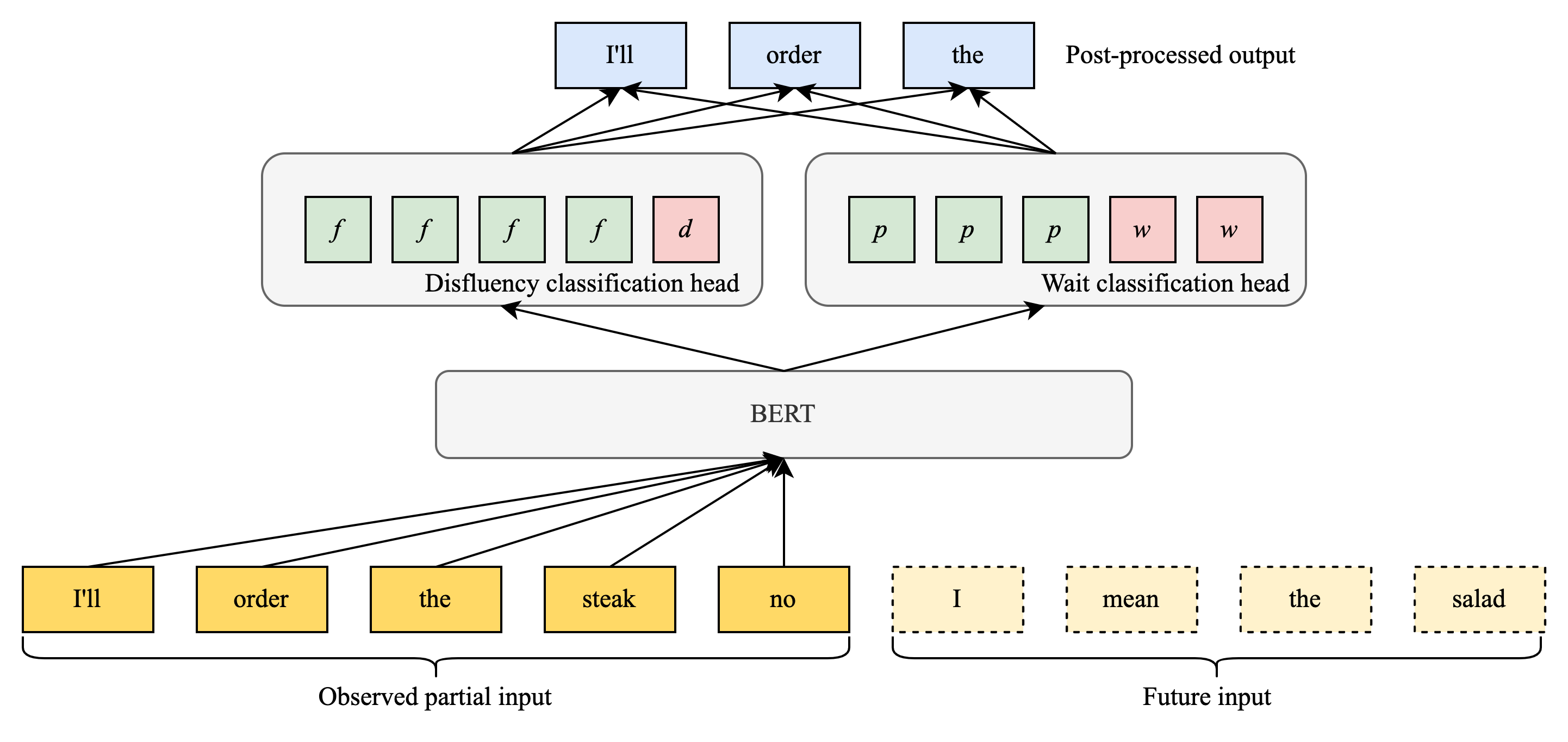
While adding this fixed look-ahead did improve the stability and streaming F1 scores in many contexts, we found that in some cases the label was already clear even without looking ahead to the next token and the model did not necessarily benefit from waiting. Other times, waiting for just one extra token was sufficient. We hypothesized that the model itself could learn when it should wait for more context. Our solution was a modified model architecture that includes a “wait” classification head that decides when the model has seen enough evidence to trust the disfluency classification head.

Diagram showing how the model labels input tokens as they arrive. The BERT embedding layers feed into two separate classification heads, which are combined for the output.

We constructed a training loss function that is a weighted sum of three factors:

  1. The traditional cross-entropy loss for the disfluency classification head
  2. A cross-entropy term that only considers up to the first token with a “wait” classification
  3. A latency penalty that discourages the model from waiting too long to make a prediction

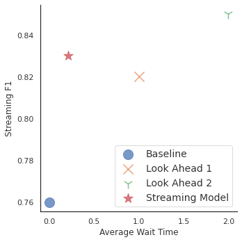
We evaluated this streaming model as well as the standard baseline with no look-ahead and with both 1- and 2-token look-ahead values:

Graph of the streaming F1 score versus the average wait time in tokens. Three data points indicate F1 scores above 0.82 across multiple wait times. The proposed streaming model achieves near top performance with much shorter wait times than the fixed look ahead models.

The streaming model achieved a better streaming F1 score than both a standard baseline with no look ahead and a model with a look ahead of 1. It performed nearly as well as the variant with fixed look ahead of 2, but with much less waiting. On average the model waited for only 0.21 tokens of context.

Internationalization
Our best outcomes so far have been with English transcripts. This is mostly due to resourcing issues: while there are a number of relatively large labeled conversational datasets that include disfluencies in English, other languages often have very few such datasets available. So, in order to make disfluency detection models available outside English a method is needed to build models in a way that does not require finding and labeling hundreds of thousands of utterances in each target language. A promising solution is to leverage multi-language versions of BERT to transfer what a model has learned about English disfluencies to other languages in order to achieve similar performance with much less data. This is an area of active research, but we do have some promising results to outline here.

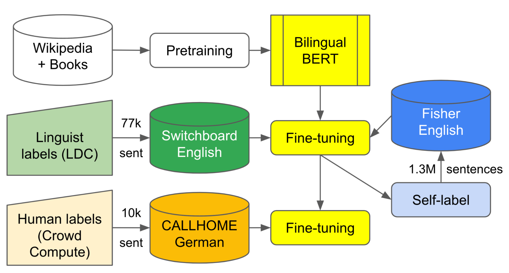
As a first effort to validate this approach, we added labels to about 10,000 lines of dialogue from the German CALLHOME dataset. We then started with the Geotrend English and German Bilingual BERT model (extracted from Multilingual BERT) and fine-tuned it with approximately 77,000 disfluency-labeled English Switchboard examples and 1.3 million examples of self-labeled transcripts from the Fisher Corpus. Then, we did further fine tuning with about 7,500 in-house–labeled examples from the German CALLHOME dataset.

Diagram illustrating the flow of labeled data and self-trained output in our best multilingual training setup. By training on both English and German data we are able to improve performance via transfer learning.

Our results indicate that fine-tuning on a large English corpus can produce acceptable precision using zero-shot transfer to similar languages like German, but at least a modest amount of German labels were needed to improve recall from less than 60% to greater than 80%. Two-stage fine-tuning of an English-German bilingual model produced the highest precision and overall F1 score.

Approach Precision Recall F1
German BERTBASE model fine-tuned on 7,300 human-labeled German CALLHOME examples 89.1% 81.3% 85.0
Same as above but with additional 7,500 self-labeled German CALLHOME examples 91.5% 83.3% 87.2
English/German Bilingual BERTbase model fine-tuned on English Switchboard+Fisher, evaluated on German CALLHOME (zero-shot language transfer) 87.2% 59.1% 70.4
Same as above but subsequently fine-tuned with 14,800 German CALLHOME (human- and self-labeled) examples 95.5% 82.6% 88.6

Conclusion
Cleaning up disfluencies from transcripts can improve not just their readability for people, but also the performance of other models that consume transcripts. We demonstrate effective methods for identifying disfluencies and expand our disfluency model to resource-constrained environments, new languages, and more interactive use cases.

Acknowledgements
Thank you to Vicky Zayats, Johann Rocholl, Angelica Chen, Noah Murad, Dirk Padfield, and Preeti Mohan for writing the code, running the experiments, and composing the papers discussed here. Wealso thank our technical product manager Aaron Schneider, Bobby Tran from the Cerebra Data Ops team, and Chetan Gupta from Speech Data Ops for their support obtaining additional data labels.

Source: Google AI Blog


Challenges in Multi-objective Optimization for Automatic Wireless Network Planning

Economics, combinatorics, physics, and signal processing conspire to make it difficult to design, build, and operate high-quality, cost-effective wireless networks. The radio transceivers that communicate with our mobile phones, the equipment that supports them (such as power and wired networking), and the physical space they occupy are all expensive, so it’s important to be judicious in choosing sites for new transceivers. Even when the set of available sites is limited, there are exponentially many possible networks that can be built. For example, given only 50 sites, there are 250 (over a million billion) possibilities!

Further complicating things, for every location where service is needed, one must know which transceiver provides the strongest signal and how strong it is. However, the physical characteristics of radio propagation in an environment containing buildings, hills, foliage, and other clutter are incredibly complex, so accurate predictions require sophisticated, computationally-intensive models. Building all possible sites would yield the best coverage and capacity, but even if this were not prohibitively expensive, it would create unacceptable interference among nearby transceivers. Balancing these trade-offs is a core mathematical difficulty.

The goal of wireless network planning is to decide where to place new transceivers to maximize coverage and capacity while minimizing cost and interference. Building an automatic network planning system (a.k.a., auto-planner) that quickly solves national-scale problems at fine-grained resolution without compromising solution quality has been among the most important and difficult open challenges in telecom research for decades.

To address these issues, we are piloting network planning tools built using detailed geometric models derived from high-resolution geographic data, that feed into radio propagation models powered by distributed computing. This system provides fast, high-accuracy predictions of signal strength. Our optimization algorithms then intelligently sift through the exponential space of possible networks to output a small menu of candidate networks that each achieve different desirable trade-offs among cost, coverage, and interference, while ensuring enough capacity to meet demand.

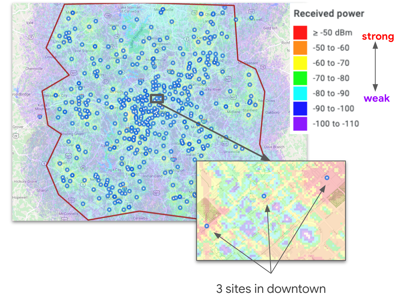
Example auto-planning project in Charlotte, NC. Blue dots denote selected candidate sites. The heat map indicates signal strength from the propagation engine. The inset emphasizes the non-isotropic path loss in downtown.

Radio Propagation
The propagation of radio waves near Earth's surface is complicated. Like ripples in a pond, they decay with distance traveled, but they can also penetrate, bounce off, or bend around obstacles, further weakening the signal. Computing radio wave attenuation across a real-world landscape (called path loss) is a hybrid process combining traditional physics-based calculations with learned corrections accounting for obstruction, diffraction, reflection, and scattering of the signal by clutter (e.g., trees and buildings).

We have developed a radio propagation modeling engine that leverages the same high-res geodata that powers Google Earth, Maps and Street View to map the 3D distribution of vegetation and buildings. While accounting for signal origin, frequency, broadcast strength, etc., we train signal correction models using extensive real-world measurements, which account for diverse propagation environments — from flat to hilly terrain and from dense urban to sparse rural areas.

While such hybrid approaches are common, using detailed geodata enables accurate path loss predictions below one-meter resolution. Our propagation engine provides fast point-to-point path loss calculations and scales massively via distributed computation. For instance, computing coverage for 25,000 transceivers scattered across the continental United States can be done at 4 meter resolution in only 1.5 hours, using 1000 CPU cores.

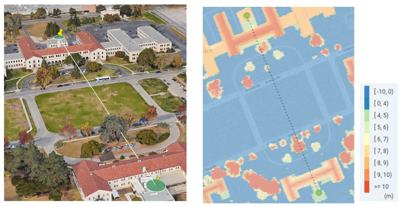
Photorealistic 3D model in Google Earth (top-left) and corresponding clutter height model (top-right). Path profile through buildings and trees from a source to destination in the clutter model (bottom). Gray denotes buildings and green denotes trees.

Auto-Planning Inputs
Once accurate coverage estimates are available, we can use them to optimize network planning, for example, deciding where to place hundreds of new sites to maximize network quality. The auto-planning solver addresses large-scale combinatorial optimization problems such as these, using a fast, robust, scalable approach.

Formally, an auto-planning input instance contains a set of demand points (usually a square grid) where service is to be provided, a set of candidate transceiver sites, predicted signal strengths from candidate sites to demand points (supplied by the propagation model), and a cost budget. Each demand point includes a demand quantity (e.g., estimated from the population of wireless users), and each site includes a cost and capacity. Signal strengths below some threshold are omitted. Finally, the input may include an overall cost budget.

Data Summarization for Large Instances
Auto-planning inputs can be huge, not just because of the number of candidate sites (tens of thousands), and demand points (billions), but also because it requires signal strengths to all demand points from all nearby candidate sites. Simple downsampling is insufficient because population density may vary widely over a given region. Therefore, we apply methods like priority sampling to shrink the data. This technique produces a low-variance, unbiased estimate of the original data, preserving an accurate view of the network traffic and interference statistics, and shrinking the input data enough that a city-size instance fits into memory on one machine.

Multi-objective Optimization via Local Search
Combinatorial optimization remains a difficult task, so we created a domain-specific local search algorithm to optimize network quality. The local search algorithmic paradigm is widely applied to address computationally-hard optimization problems. Such algorithms move from one solution to another through a search space of candidate solutions by applying small local changes, stopping at a time limit or when the solution is locally optimal. To evaluate the quality of a candidate network, we combine the different objective functions into a single one, as described in the following section.

The number of local steps to reach a local optimum, number of candidate moves we evaluate per step, and time to evaluate each candidate can all be large when dealing with realistic networks. To achieve a high-quality algorithm that finishes within hours (rather than days), we must address each of these components. Fast candidate evaluation benefits greatly from dynamic data structures that maintain the mapping between each demand point and the site in the candidate solution that provides the strongest signal to it. We update this “strongest-signal” map efficiently as the candidate solution evolves during local search. The following observations help limit both the number of steps to convergence and evaluations per step.

Bipartite graph representing candidate sites (left) and demand points (right). Selected sites are circled in red, and each demand point is assigned to its strongest available connection. The topmost demand point has no service because the only site that can reach it was not selected. The third and fourth demand points from the top may have high interference if the signal strengths attached to their gray edges are only slightly lower than the ones on their red edges. The bottommost site has high congestion because many demand points get their service from that site, possibly exceeding its capacity.

Selecting two nearby sites is usually not ideal because they interfere. Our algorithm explicitly forbids such pairs of sites, thereby steering the search toward better solutions while greatly reducing the number of moves considered per step. We identify pairs of forbidden sites based on the demand points they cover, as measured by the weighted Jaccard index. This captures their functional proximity much better than simple geographic distance does, especially in urban or hilly areas where radio propagation is highly non-isotropic.

Breaking the local search into epochs also helps. The first epoch mostly adds sites to increase the coverage area while avoiding forbidden pairs. As we approach the cost budget, we begin a second epoch that includes swap moves between forbidden pairs to fine-tune the interference. This restriction limits the number of candidate moves per step, while focusing on those that improve interference with less change to coverage.

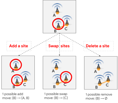
Three candidate local search moves. Red circles indicate selected sites and the orange edge indicates a forbidden pair.

Outputting a Diverse Set of Good Solutions
As mentioned before, auto-planning must balance three competing objectives: maximizing coverage, while minimizing interference and capacity violations, subject to a cost budget. There is no single correct tradeoff, so our algorithm delegates the final decision to the user by providing a small menu of candidate networks with different emphases. We apply a multiplier to each objective and optimize the sum. Raising the multiplier for a component guides the algorithm to emphasize it. We perform grid search over multipliers and budgets, generating a large number of solutions, filter out any that are worse than another solution along all four components (including cost), and finally select a small subset that represent different tradeoffs.

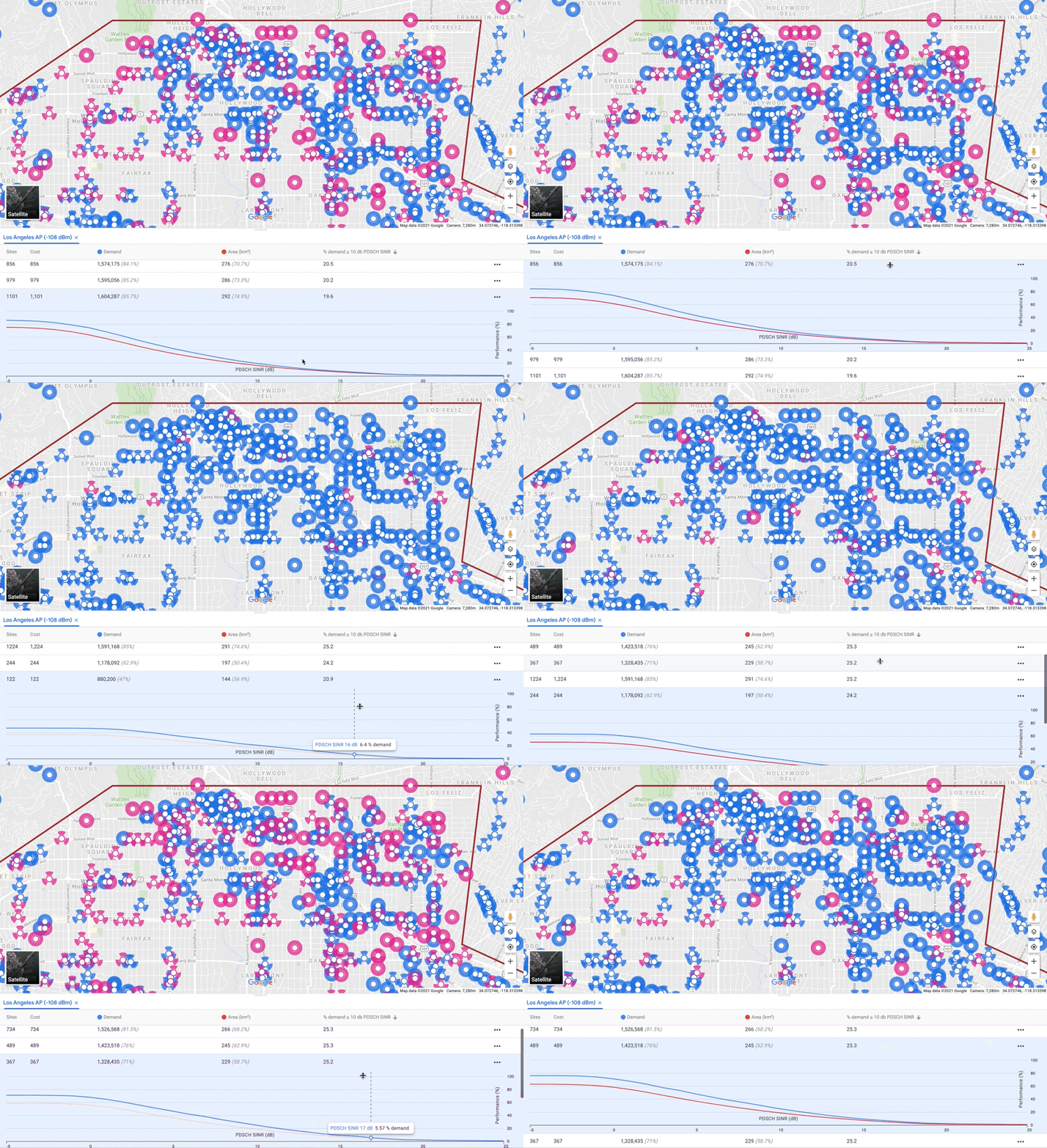
Menu of candidate solutions, one per row, displaying metrics. Clicking on a solution turns the selected sites pink and displays a plot of the interference distribution across covered area and demand. Sites not selected are blue.

Conclusion
We described our efforts to address the most vexing challenges facing telecom network operators. Using combinatorial optimization in concert with geospatial and radio propagation modeling, we built a scalable auto-planner for wireless telecommunication networks. We are actively exploring how to expand these capabilities to best meet the needs of our customers. Stay tuned!

For questions and other inquiries, please reach out to [email protected].

Acknowledgements
These technological advances were enabled by the tireless work of our collaborators: Aaron Archer, Serge Barbosa Da Torre, Imad Fattouch, Danny Liberty, Pishoy Maksy, Zifei Tong, and Mat Varghese. Special thanks to Corinna Cortes, Mazin Gilbert, Rob Katcher, Michael Purdy, Bea Sebastian, Dave Vadasz, Josh Williams, and Aaron Yonas, along with Serge and especially Aaron Archer for their assistance with this blog post.

Source: Google AI Blog


Learning Locomotion Skills Safely in the Real World

The promise of deep reinforcement learning (RL) in solving complex, high-dimensional problems autonomously has attracted much interest in areas such as robotics, game playing, and self-driving cars. However, effectively training an RL policy requires exploring a large set of robot states and actions, including many that are not safe for the robot. This is a considerable risk, for example, when training a legged robot. Because such robots are inherently unstable, there is a high likelihood of the robot falling during learning, which could cause damage.

The risk of damage can be mitigated to some extent by learning the control policy in computer simulation and then deploying it in the real world. However, this approach usually requires addressing the difficult sim-to-real gap, i.e., the policy trained in simulation can not be readily deployed in the real world for various reasons, such as sensor noise in deployment or the simulator not being realistic enough during training. Another approach to solve this issue is to directly learn or fine-tune a control policy in the real world. But again, the main challenge is to assure safety during learning.

In “Safe Reinforcement Learning for Legged Locomotion”, we introduce a safe RL framework for learning legged locomotion while satisfying safety constraints during training. Our goal is to learn locomotion skills autonomously in the real world without the robot falling during the entire learning process. Our learning framework adopts a two-policy safe RL framework: a “safe recovery policy” that recovers robots from near-unsafe states, and a “learner policy” that is optimized to perform the desired control task. The safe learning framework switches between the safe recovery policy and the learner policy to enable robots to safely acquire novel and agile motor skills.

The Proposed Framework
Our goal is to ensure that during the entire learning process, the robot never falls, regardless of the learner policy being used. Similar to how a child learns to ride a bike, our approach teaches an agent a policy while using "training wheels", i.e., a safe recovery policy. We first define a set of states, which we call a “safety trigger set”, where the robot is close to violating safety constraints but can still be saved by a safe recovery policy. For example, the safety trigger set can be defined as a set of states with the height of the robots being below a certain threshold and the roll, pitch, yaw angles being too large, which is an indication of falls. When the learner policy results in the robot being within the safety trigger set (i.e., where it is likely to fall), we switch to the safe recovery policy, which drives the robot back to a safe state. We determine when to switch back to the learner policy by leveraging an approximate dynamics model of the robot to predict the future robot trajectory. For example, based on the position of the robot’s legs and the current angle of the robot based on sensors for roll, pitch, and yaw, is it likely to fall in the future? If the predicted future states are all safe, we hand the control back to the learner policy, otherwise, we keep using the safe recovery policy.

The state diagram of the proposed approach. (1) If the learner policy violates the safety constraint, we switch to the safe recovery policy. (2) If the learner policy cannot ensure safety in the near future after switching to the safe recovery policy, we keep using the safe recovery policy. This allows the robot to explore more while ensuring safety.

This approach ensures safety in complex systems without resorting to opaque neural networks that may be sensitive to distribution shifts in application. In addition, the learner policy is able to explore states that are near safety violations, which is useful for learning a robust policy.

Because we use “approximated” dynamics to predict the future trajectory, we also examine how much safer a robot would be if we used a much more accurate model for its dynamics. We provide a theoretical analysis of this problem and show that our approach can achieve minimal safety performance loss compared to one with a full knowledge about the system dynamics.

Legged Locomotion Tasks
To demonstrate the effectiveness of the algorithm, we consider learning three different legged locomotion skills:

  1. Efficient Gait: The robot learns how to walk with low energy consumption and is rewarded for consuming less energy.
  2. Catwalk: The robot learns a catwalk gait pattern, in which the left and right two feet are close to each other. This is challenging because by narrowing the support polygon, the robot becomes less stable.
  3. Two-leg Balance: The robot learns a two-leg balance policy, in which the front-right and rear-left feet are in stance, and the other two are lifted. The robot can easily fall without delicate balance control because the contact polygon degenerates into a line segment.
Locomotion tasks considered in the paper. Top: efficient gait. Middle: catwalk. Bottom: two-leg balance.

Implementation Details
We use a hierarchical policy framework that combines RL and a traditional control approach for the learner and safe recovery policies. This framework consists of a high-level RL policy, which produces gait parameters (e.g., stepping frequency) and feet placements, and pairs it with a low-level process controller called model predictive control (MPC) that takes in these parameters and computes the desired torque for each motor in the robot. Because we do not directly command the motors’ angles, this approach provides more stable operation, streamlines the policy training due to a smaller action space, and results in a more robust policy. The input of the RL policy network includes the previous gait parameters, the height of the robot, base orientation, linear, angular velocities, and feedback to indicate whether the robot is approaching the safety trigger set. We use the same setup for each task.

We train a safe recovery policy with a reward for reaching stability as soon as possible. Furthermore, we design the safety trigger set with inspiration from capturability theory. In particular, the initial safety trigger set is defined to ensure that the robot’s feet can not fall outside of the positions from which the robot can safely recover using the safe recovery policy. We then fine-tune this set on the real robot with a random policy to prevent the robot from falling.

Real-World Experiment Results
We report the real-world experimental results showing the reward learning curves and the percentage of safe recovery policy activations on the efficient gait, catwalk, and two-leg balance tasks. To ensure that the robot can learn to be safe, we add a penalty when triggering the safe recovery policy. Here, all the policies are trained from scratch, except for the two-leg balance task, which was pre-trained in simulation because it requires more training steps.

Overall, we see that on these tasks, the reward increases, and the percentage of uses of the safe recovery policy decreases over policy updates. For instance, the percentage of uses of the safe recovery policy decreases from 20% to near 0% in the efficient gait task. For the two-leg balance task, the percentage drops from near 82.5% to 67.5%, suggesting that the two-leg balance is substantially harder than the previous two tasks. Still, the policy does improve the reward. This observation implies that the learner can gradually learn the task while avoiding the need to trigger the safe recovery policy. In addition, this suggests that it is possible to design a safe trigger set and a safe recovery policy that does not impede the exploration of the policy as the performance increases.

The reward learning curve (blue) and the percentage of safe recovery policy activations (red) using our safe RL algorithm in the real world.

In addition, the following video shows the learning process for the two-leg balance task, including the interplay between the learner policy and the safe recovery policy, and the reset to the initial position when an episode ends. We can see that the robot tries to catch itself when falling by putting down the lifted legs (front left and rear right) outward, creating a support polygon. After the learning episode ends, the robot walks back to the reset position automatically. This allows us to train policy autonomously and safely without human supervision.

Early training stage.
Late training stage.
Without a safe recovery policy.

Finally, we show the clips of learned policies. First, in the catwalk task, the distance between two sides of the legs is 0.09m, which is 40.9% smaller than the nominal distance. Second, in the two-leg balance task, the robot can maintain balance by jumping up to four times via two legs, compared to one jump from the policy pre-trained from simulation.

Final learned two-leg balance.

Conclusion
We presented a safe RL framework and demonstrated how it can be used to train a robotic policy with no falls and without the need for a manual reset during the entire learning process for the efficient gait and catwalk tasks. This approach even enables training of a two-leg balance task with only four falls. The safe recovery policy is triggered only when needed, allowing the robot to more fully explore the environment. Our results suggest that learning legged locomotion skills autonomously and safely is possible in the real world, which could unlock new opportunities including offline dataset collection for robot learning.

No model is without limitation. We currently ignore the model uncertainty from the environment and non-linear dynamics in our theoretical analysis. Including these would further improve the generality of our approach. In addition, some hyper-parameters of the switching criteria are currently being heuristically tuned. It would be more efficient to automatically determine when to switch based on the learning progress. Furthermore, it would be interesting to extend this safe RL framework to other robot applications, such as robot manipulation. Finally, designing an appropriate reward when incorporating the safe recovery policy can impact learning performance. We use a penalty-based approach that obtained reasonable results in these experiments, but we plan to investigate this in future work to make further performance improvements.

Acknowledgements
We would like to thank our paper co-authors: Tingnan Zhang, Linda Luu, Sehoon Ha, Jie Tan, and Wenhao Yu. We would also like to thank the team members of Robotics at Google for discussions and feedback.

Source: Google AI Blog