Posted by Kostas Kollias and Sreenivas Gollapudi, Research Scientists, Geo Algorithms Team, Google Research
Mapping algorithms used for navigation often rely on Dijkstra’s algorithm, a fundamental textbook solution for finding shortest paths in graphs. Dijkstra’s algorithm is simple and elegant -- rather than considering all possible routes (an exponential number) it iteratively improves an initial solution, and works in polynomial time. The original algorithm and practical extensions of it (such as the A* algorithm) are used millions of times per day for routing vehicles on the global road network. However, due to the fact that most vehicles are gas-powered, these algorithms ignore refueling considerations because a) gas stations are usually available everywhere at the cost of a small detour, and b) the time needed to refuel is typically only a few minutes and is negligible compared to the total travel time.
This situation is different for electric vehicles (EVs). First, EV charging stations are not as commonly available as gas stations, which can cause range anxiety, the fear that the car will run out of power before reaching a charging station. This concern is common enough that it is considered one of the barriers to the widespread adoption of EVs. Second, charging an EV’s battery is a more decision-demanding task, because the charging time can be a significant fraction of the total travel time and can vary widely by station, vehicle model, and battery level. In addition, the charging time is non-linear — e.g., it takes longer to charge a battery from 90% to 100% than from 20% to 30%.
The EV can only travel a distance up to the illustrated range before needing to recharge. Different roads and different stations have different time costs. The goal is to optimize for the total trip time.
Today, we present a new approach for routing of EVs integrated into the latest release of Google Maps built into your car for participating EVs that reduces range anxiety by integrating recharging stations into the navigational route. Based on the battery level and the destination, Maps will recommend the charging stops and the corresponding charging levels that will minimize the total duration of the trip. To accomplish this we engineered a highly scalable solution for recommending efficient routes through charging stations, which optimizes the sum of the driving time and the charging time together.
The fastest route from Berlin to Paris for a gas fueled car is shown in the top figure. The middle figure shows the optimal route for a 400 km range EV (travel time indicated - charging time excluded), where the larger white circles along the route indicate charging stops. The bottom figure shows the optimal route for a 200 km range EV.
Routing Through Charging Stations A fundamental constraint on route selection is that the distance between recharging stops cannot be higher than what the vehicle can reach on a full charge. Consequently, the route selection model emphasizes the graph of charging stations, as opposed to the graph of road segments of the road network, where each charging station is a node and each trip between charging stations is an edge. Taking into consideration the various characteristics of each EV (such as the weight, maximum battery level, plug type, etc.) the algorithm identifies which of the edges are feasible for the EV under consideration and which are not. Once the routing request comes in, Maps EV routing augments the feasible graph with two new nodes, the origin and the destination, and with multiple new (feasible) edges that outline the potential trips from the origin to its nearby charging stations and to the destination from each of its nearby charging stations.
Routing using Dijkstra’s algorithm or A* on this graph is sufficient to give a feasible solution that optimizes for the travel time for drivers that do not care at all about the charging time, (i.e., drivers who always fully charge their batteries at each charging station). However, such algorithms are not sufficient to account for charging times. In this case, the algorithm constructs a new graph by replicating each charging station node multiple times. Half of the copies correspond to entering the station with a partially charged battery, with a charge, x, ranging from 0%-100%. The other half correspond to exiting the station with a fractional charge, y (again from 0%-100%). We add an edge from the entry node at the charge x to the exit node at charge y (constrained by y > x), with a corresponding charging time to get from x to y. When the trip from Station A to Station B spends some fraction (z) of the battery charge, we introduce an edge between every exit node of Station A to the corresponding entry node of Station B (at charge x-z). After performing this transformation, using Dijkstra or A* recovers the solution.
An example of our node/edge replication. In this instance the algorithm opts to pass through the first station without charging and charges at the second station from 20% to 80% battery.
Graph Sparsification To perform the above operations while addressing range anxiety with confidence, the algorithm must compute the battery consumption of each trip between stations with good precision. For this reason, Maps maintains detailed information about the road characteristics along the trip between any two stations (e.g., the length, elevation, and slope, for each segment of the trip), taking into consideration the properties of each type of EV.
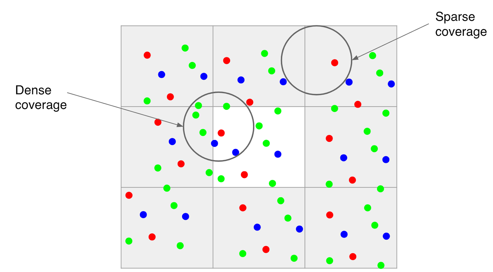
Due to the volume of information required for each segment, maintaining a large number of edges can become a memory intensive task. While this is not a problem for areas where EV charging stations are sparse, there exist locations in the world (such as Northern Europe) where the density of stations is very high. In such locations, adding an edge for every pair of stations between which an EV can travel quickly grows to billions of possible edges.
The figure on the left illustrates the high density of charging stations in Northern Europe. Different colors correspond to different plug types. The figure on the right illustrates why the routing graph scales up very quickly in size as the density of stations increases. When there are many stations within range of each other, the induced routing graph is a complete graph that stores detailed information for each edge.
However, this high density implies that a trip between two stations that are relatively far apart will undoubtedly pass through multiple other stations. In this case, maintaining information about the long edge is redundant, making it possible to simply add the smaller edges (spanners) in the graph, resulting in sparser, more computationally feasible, graphs.
The spanner construction algorithm is a direct generalization of the greedy geometric spanner. The trips between charging stations are sorted from fastest to slowest and are processed in that order. For each trip between points a and b, the algorithm examines whether smaller subtrips already included in the spanner subsume the direct trip. To do so it compares the trip time and battery consumption that can be achieved using subtrips already in the spanner, against the same quantities for the direct a-b route. If they are found to be within a tiny error threshold, the direct trip from a to b is not added to the spanner, otherwise it is. Applying this sparsification algorithm has a notable impact and allows the graph to be served efficiently in responding to users’ routing requests.
On the left is the original road network (EV stations in light red). The station graph in the middle has edges for all feasible trips between stations. The sparse graph on the right maintains the distances with much fewer edges.
Summary In this work we engineer a scalable solution for routing EVs on long trips to include access to charging stations through the use of graph sparsification and novel framing of standard routing algorithms. We are excited to put algorithmic ideas and techniques in the hands of Maps users and look forward to serving stress-free routes for EV drivers across the globe!
Acknowledgements We thank our collaborators Dixie Wang, Xin Wei Chow, Navin Gunatillaka, Stephen Broadfoot, Alex Donaldson, and Ivan Kuznetsov.
Posted by Badih Ghazi and Joshua R. Wang, Research Scientists, Google Research
Much of classical machine learning (ML) focuses on utilizing available data to make more accurate predictions. More recently, researchers have considered other important objectives, such as how to design algorithms to be small, efficient, and robust. With these goals in mind, a natural research objective is the design of a system on top of neural networks that efficiently stores information encoded within—in other words, a mechanism to compute a succinct summary (a “sketch”) of how a complex deep network processes its inputs. Sketching is a rich field of study that dates back to the foundational work of Alon, Matias, and Szegedy, which can enable neural networks to efficiently summarize information about their inputs.
For example: Imagine stepping into a room and briefly viewing the objects within. Modern machine learning is excellent at answering immediate questions, known at training time, about this scene: “Is there a cat? How big is said cat?” Now, suppose we view this room every day over the course of a year. People can reminisce about the times they saw the room: “How often did the room contain a cat? Was it usually morning or night when we saw the room?”. However, can one design systems that are also capable of efficiently answering such memory-based questions even if they are unknown at training time?
In “Recursive Sketches for Modular Deep Learning”, recently presented at ICML 2019, we explore how to succinctly summarize how a machine learning model understands its input. We do this by augmenting an existing (already trained) machine learning model with “sketches” of its computation, using them to efficiently answer memory-based questions—for example, image-to-image-similarity and summary statistics—despite the fact that they take up much less memory than storing the entire original computation.
Basic Sketching Algorithms In general, sketching algorithms take a vector x and produce an output sketch vector that behaves like x but whose storage cost is much smaller. The fact that the storage cost is much smaller allows one to succinctly store information about the network, which is critical for efficiently answering memory-based questions. In the simplest case, a linear sketch x is given by the matrix-vector product Ax where A is a wide matrix, i.e., the number of columns is equal to the original dimension of x and the number of rows is equal to the new reduced dimension. Such methods have led to a variety of efficient algorithms for basic tasks on massive datasets, such as estimating fundamental statistics (e.g., histogram, quantiles and interquartile range), finding popular items (known as frequent elements), as well as estimating the number of distinct elements (known as support size) and the related tasks of norms and entropy estimation.
A simple method to sketch the vector x is to multiply it by a wide matrix A to produce a lower-dimensional vector y.
This basic approach works well in the relatively simple case of linear regression, where it is possible to identify important data dimensions simply by the magnitude of weights (under the common assumption that they have uniform variance). However, many modern machine learning models are actually deep neural networks and are based on high-dimensional embeddings (such as Word2Vec, Image Embeddings, Glove, DeepWalk and BERT), which makes the task of summarizing the operation of the model on the input much more difficult. However, a large subset of these more complex networks are modular, allowing us to generate accurate sketches of their behavior, in spite of their complexity.
Neural Network Modularity A modular deep network consists of several independent neural networks (modules) that only communicate via one’s output serving as another’s input. This concept has inspired several practical architectures, including Neural Modular Networks, Capsule Neural Networks and PathNet. It is also possible to split other canonical architectures to view them as modular networks and apply our approach. For example, convolutional neural networks (CNNs) are traditionally understood to behave in a modular fashion; they detect basic concepts and attributes in their lower layers and build up to detecting more complex objects in their higher layers. In this view, the convolution kernels correspond to modules. A cartoon depiction of a modular network is given below.
This is a cartoon depiction of a modular network for image processing. Data flows from the bottom of the figure to the top through the modules represented with blue boxes. Note that modules in the lower layers correspond to basic objects, such as edges in an image, while modules in upper layers correspond to more complex objects, like humans or cats. Also notice that in this imaginary modular network, the output of the face module is generic enough to be used by both the human and cat modules.
Sketch Requirements To optimize our approach for these modular networks, we identified several desired properties that a network sketch should satisfy:
Sketch-to-Sketch Similarity: The sketches of two unrelated network operations (either in terms of the present modules or in terms of the attribute vectors) should be very different; on the other hand, the sketches of two similar network operations should be very close.
Attribute Recovery: The attribute vector, e.g., the activations of any node of the graph can be approximately recovered from the top-level sketch.
Summary Statistics: If there are multiple similar objects, we can recover summary statistics about them. For example, if an image has multiple cats, we can count how many there are. Note that we want to do this without knowing the questions ahead of time.
Graceful Erasure: Erasing a suffix of the top-level sketch maintains the above properties (but would smoothly increase the error).
Network Recovery: Given sufficiently many (input, sketch) pairs, the wiring of the edges of the network as well as the sketch function can be approximately recovered.
This is a 2D cartoon depiction of the sketch-to-sketch similarity property. Each vector represents a sketch and related sketches are more likely to cluster together.
The Sketching Mechanism The sketching mechanism we propose can be applied to a pre-trained modular network. It produces a single top-level sketch summarizing the operation of this network, simultaneously satisfying all of the desired properties above. To understand how it does this, it helps to first consider a one-layer network. In this case, we ensure that all the information pertaining to a specific node is “packed” into two separate subspaces, one corresponding to the node itself and one corresponding to its associated module. Using suitable projections, the first subspace lets us recover the attributes of the node whereas the second subspace facilitates quick estimates of summary statistics. Both subspaces help enforce the aforementioned sketch-to-sketch similarity property. We demonstrate that these properties hold if all the involved subspaces are chosen independently at random.
Of course, extra care has to be taken when extending this idea to networks with more than one layer—which leads to our recursive sketching mechanism. Due to their recursive nature, these sketches can be “unrolled” to identify sub-components, capturing even complicated network structures. Finally, we utilize a dictionary learning algorithm tailored to our setup to prove that the random subspaces making up the sketching mechanism together with the network architecture can be recovered from a sufficiently large number of (input, sketch) pairs.
Future Directions The question of succinctly summarizing the operation of a network seems to be closely related to that of model interpretability. It would be interesting to investigate whether ideas from the sketching literature can be applied to this domain. Our sketches could also be organized in a repository to implicitly form a “knowledge graph”, allowing patterns to be identified and quickly retrieved. Moreover, our sketching mechanism allows for seamlessly adding new modules to the sketch repository—it would be interesting to explore whether this feature can have applications to architecture search and evolving network topologies. Finally, our sketches can be viewed as a way of organizing previously encountered information in memory, e.g., images that share the same modules or attributes would share subcomponents of their sketches. This, on a very high level, is similar to the way humans use prior knowledge to recognize objects and generalize to unencountered situations.
Acknowledgements This work was the joint effort of Badih Ghazi, Rina Panigrahy and Joshua R. Wang.
Posted by Alex Ratner, Stanford University and Cassandra Xia, Google AI
One of the biggest bottlenecks in developing machine learning (ML) applications is the need for the large, labeled datasets used to train modern ML models. Creating these datasets involves the investment of significant time and expense, requiring annotators with the right expertise. Moreover, due to the evolution of real-world applications, labeled datasets often need to be thrown out or re-labeled.
In collaboration with Stanford and Brown University, we present "Snorkel Drybell: A Case Study in Deploying Weak Supervision at Industrial Scale," which explores how existing knowledge in an organization can be used as noisier, higher-level supervision—or, as it is often termed, weak supervision—to quickly label large training datasets. In this study, we use an experimental internal system, Snorkel Drybell, which adapts the open-source Snorkel framework to use diverse organizational knowledge resources—like internal models, ontologies, legacy rules, knowledge graphs and more—in order to generate training data for machine learning models at web scale. We find that this approach can match the efficacy of hand-labeling tens of thousands of data points, and reveals some core lessons about how training datasets for modern machine learning models can be created in practice.
Rather than labeling training data by hand, Snorkel DryBell enables writing labeling functions that label training data programmatically. In this work, we explored how these labeling functions can capture engineers' knowledge about how to use existing resources as heuristics for weak supervision. As an example, suppose our goal is to identify content related to celebrities. One can leverage an existing named-entity recognition (NER) model for this task by labeling any content that does not contain a person as not related to celebrities. This illustrates how existing knowledge resources (in this case, a trained model) can be combined with simple programmatic logic to label training data for a new model. Note also, importantly, that this labeling function returns None---i.e. abstains---in many cases, and thus only labels some small part of the data; our overall goal is to use these labels to train a modern machine learning model that can generalize to new data.
In our example of a labeling function, rather than hand-labeling a data point (1), one utilizes an existing knowledge resource—in this case, a NER model (2)—together with some simple logic expressed in code (3) to heuristically label data.
This programmatic interface for labeling training data is much faster and more flexible than hand-labeling individual data points, but the resulting labels are obviously of much lower quality than manually-specified labels. The labels generated by these labeling functions will often overlap and disagree, as the labeling functions may not only have arbitrary unknown accuracies, but may also be correlated in arbitrary ways (for example, from sharing a common data source or heuristic).
To solve the problem of noisy and correlated labels, Snorkel DryBell uses a generative modeling technique to automatically estimate the accuracies and correlations of the labeling functions in a provably consistent way—without any ground truth training labels—then uses this to re-weight and combine their outputs into a single probabilistic label per data point. At a high level, we rely on the observed agreements and disagreements between the labeling functions (the covariance matrix), and learn the labeling function accuracy and correlation parameters that best explain this observed output using a new matrix completion-style approach. The resulting labels can then be used to train an arbitrary model (e.g. in TensorFlow), as shown in the system diagram below.
Using Diverse Knowledge Sources as Weak Supervision To study the efficacy of Snorkel Drybell, we used three production tasks and corresponding datasets, aimed at classifying topics in web content, identifying mentions of certain products, and detecting certain real-time events. Using Snorkel DryBell, we were able to make use of various existing or quickly specified sources of information such as:
Heuristics and rules: e.g. existing human-authored rules about the target domain.
Topic models, taggers, and classifiers: e.g. machine learning models about the target domain or a related domain.
Aggregate statistics: e.g. tracked metrics about the target domain.
Knowledge or entity graphs: e.g. databases of facts about the target domain.
In Snorkel DryBell, the goal is to train a machine learning model (C), for example to do content or event classification over web data. Rather than hand-labeling training data to do this, in Snorkel DryBell users write labeling functions that express various organizational knowledge resources (A), which are then automatically reweighted and combined (B).
We used these organizational knowledge resources to write labeling functions in a MapReduce template-based pipeline. Each labeling function takes in a data point and either abstains, or outputs a label. The result is a large set of programmatically-generated training labels. However, many of these labels were very noisy (e.g. from the heuristics), conflicted with each other, or were far too coarse-grained (e.g. the topic models) for our task, leading to the next stage of Snorkel DryBell, aimed at automatically cleaning and integrating the labels into a final training set.
Modeling the Accuracies to Combine & Repurpose Existing Sources To handle these noisy labels, the next stage of Snorkel DryBell combines the outputs from the labeling functions into a single, confidence-weighted training label for each data point. The challenging technical aspect is that this must be done without any ground-truth labels. We use a generative modeling technique that learns the accuracy of each labeling function using only unlabeled data. This technique learns by observing the matrix of agreements and disagreements between the labeling functions' outputs, taking into account known (or statistically estimated) correlation structures between them. In Snorkel DryBell, we also implement a new faster, sampling-free version of this modeling approach, implemented in TensorFlow, in order to handle web-scale data.
By combining and modeling the output of the labeling functions using this procedure in Snorkel DryBell, we were able to generate high-quality training labels. In fact, on the two applications where hand-labeled training data was available for comparison, we achieved the same predictive accuracy training a model with Snorkel DryBell's labels as we did when training that same model with 12,000 and 80,000 hand-labeled training data points.
Transferring Non-Servable Knowledge to Servable Models In many settings, there is also an important distinction between servable features—which can be used in production—and non-servable features, that are too slow or expensive to be used in production. These non-servable features may have very rich signal, but a general question is how to use them to train or otherwise help servable models that can be deployed in production?
In many settings, users write labeling functions that leverage organizational knowledge resources that are not servable in production (a)—e.g. aggregate statistics, internal models, or knowledge graphs that are too slow or expensive to use in production—in order to train models that are only defined over production-servable features (b), e.g. cheap, real-time web signals.
In Snorkel DryBell, we found that users could write the labeling functions—i.e. express their organizational knowledge—over one feature set that was not servable, and then use the resulting training labels output by Snorkel DryBell to train a model defined over a different, servable feature set. This cross-feature transfer boosted our performance by an average 52% on the benchmark datasets we created. More broadly, it represents a simple but powerful way to use resources that are too slow (e.g. expensive models or aggregate statistics), private (e.g. entity or knowledge graphs), or otherwise unsuitable for deployment, to train servable models over cheap, real-time features. This approach can be viewed as a new type of transfer learning, where instead of transferring a model between different datasets, we're transferring domain knowledge between different feature sets- an approach which has potential use cases not just in industry, but in medical settings and beyond.
Next Steps Moving forward, we're excited to see what other types of organizational knowledge can be used as weak supervision, and how the approach used by Snorkel DryBell can enable new modes of information reuse and sharing across organizations. For more details, check out our paper, and for further technical details, blog posts, and tutorials, check out the open-source Snorkel implementation at snorkel.stanford.edu.
Acknowledgments This research was done in collaboration between Google, Stanford, and Brown. We would like to thank all the people who were involved, including Stephen Bach (Brown), Daniel Rodriguez, Yintao Liu, Chong Luo, Haidong Shao, Souvik Sen, Braden Hancock (Stanford), Houman Alborzi, Rahul Kuchhal, Christopher Ré (Stanford), Rob Malkin.
Posted by Charles Weill, Software Engineer, Google AI, NYC
Ensemble learning, the art of combining different machine learning (ML) model predictions, is widely used with neural networks to achieve state-of-the-art performance, benefitting from a rich history and theoretical guarantees to enable success at challenges such as the Netflix Prize and various Kaggle competitions. However, they aren’t used much in practice due to long training times, and the ML model candidate selection requires its own domain expertise. But as computational power and specialized deep learning hardware such as TPUs become more readily available, machine learning models will grow larger and ensembles will become more prominent. Now, imagine a tool that automatically searches over neural architectures, and learns to combine the best ones into a high-quality model.
Today, we’re excited to share AdaNet, a lightweight TensorFlow-based framework for automatically learning high-quality models with minimal expert intervention. AdaNet builds on our recent reinforcement learning and evolutionary-based AutoML efforts to be fast and flexible while providing learning guarantees. Importantly, AdaNet provides a general framework for not only learning a neural network architecture, but also for learning to ensemble to obtain even better models.
AdaNet is easy to use, and creates high-quality models, saving ML practitioners the time normally spent selecting optimal neural network architectures, implementing an adaptive algorithm for learning a neural architecture as an ensemble of subnetworks. AdaNet is capable of adding subnetworks of different depths and widths to create a diverse ensemble, and trade off performance improvement with the number of parameters.
AdaNet adaptively growing an ensemble of neural networks. At each iteration, it measures the ensemble loss for each candidate, and selects the best one to move onto the next iteration.
Fast and Easy to Use AdaNet implements the TensorFlow Estimator interface, which greatly simplifies machine learning programming by encapsulating training, evaluation, prediction and export for serving. It integrates with open-source tools like TensorFlow Hub modules, TensorFlow Model Analysis, and Google Cloud’s Hyperparameter Tuner. Distributed training support significantly reduces training time, and scales linearly with available CPUs and accelerators (e.g. GPUs).
AdaNet’s accuracy (y-axis) per train step (x-axis) on CIFAR-100. The blue line is accuracy on the training set, and red line is performance on the test set. A new subnetwork begins training every million steps, and eventually improves the performance of the ensemble. The grey and green lines are the accuracies of the ensemble before adding the new subnetwork.
Because TensorBoard is one of the best TensorFlow features for visualizing model metrics during training, AdaNet integrates seamlessly with it in order to monitor subnetwork training, ensemble composition, and performance. When AdaNet is done training, it exports a SavedModel that can be deployed with TensorFlow Serving.
Learning Guarantees Building an ensemble of neural networks has several challenges: What are the best subnetwork architectures to consider? Is it best to reuse the same architectures or encourage diversity? While complex subnetworks with more parameters will tend to perform better on the training set, they may not generalize to unseen data due to their greater complexity. These challenges stem from evaluating model performance. We could evaluate performance on a hold-out set split from the training set, but in doing so would reduce the number of examples one can use for training the neural network.
Instead, AdaNet’s approach (presented in “AdaNet: Adaptive Structural Learning of Artificial Neural Networks” at ICML 2017) is to optimize an objective that balances the trade-offs between the ensemble’s performance on the training set and its ability to generalize to unseen data. The intuition is for the ensemble to include a candidate subnetwork only when it improves the ensemble’s training loss more than it affects its ability to generalize. This guarantees that:
The generalization error of the ensemble is bounded by its training error and complexity.
By optimizing this objective, we are directly minimizing this bound.
A practical benefit of optimizing this objective is that it eliminates the need for a hold-out set for choosing which candidate subnetworks to add to the ensemble. This has the added benefit of enabling the use of more training data for training the subnetworks. To learn more, please walk through our tutorial about the AdaNet objective.
Extensible We believe that the key to making a useful AutoML framework for both research and production use is to not only provide sensible defaults, but to also allow users to try their own subnetwork/model definitions. As a result, machine learning researchers, practitioners, and enthusiasts are invited to define their own AdaNet adanet.subnetwork.Builder using high level TensorFlow APIs like tf.layers.
Users who have already integrated a TensorFlow model in their system can easily convert their TensorFlow code into an AdaNet subnetwork, and use the adanet.Estimator to boost model performance while obtaining learning guarantees. AdaNet will explore their defined search space of candidate subnetworks and learn to ensemble the subnetworks. For instance, we took an open-source implementation of a NASNet-A CIFAR architecture, transformed it into a subnetwork, and improved upon CIFAR-10 state-of-the-art results after eight AdaNet iterations. Furthermore, our model achieves this result with fewer parameters:
Performance of a NASNet-A model as presented in Zoph et al., 2018 versus AdaNet learning to combine small NASNet-A subnetworks on CIFAR-10.
Users are also invited to use their own custom loss functions as part of the AdaNet objective via canned or custom tf.contrib.estimator.Heads in order to train regression, classification, and multi-task learning problems.
Users can also fully define the search space of candidate subnetworks to explore by extending the adanet.subnetwork.Generator class. This allows them to grow or reduce their search space based on their available hardware. The search space of subnetworks can be as simple as duplicating the same subnetwork configuration with different random seeds, to training dozens of subnetworks with different hyperparameter combinations, and letting AdaNet choose the one to include in the final ensemble.
If you’re interested in trying AdaNet for yourself, please check out our Github repo, and walk through the tutorial notebooks. We’ve included a few working examples using dense layers and convolutions to get you started. AdaNet is an ongoing research project, and we welcome contributions. We’re excited to see how AdaNet can help the research community.
Acknowledgements This project was only possible thanks to the members of the core team including Corinna Cortes, Mehryar Mohri, Xavi Gonzalvo, Charles Weill, Vitaly Kuznetsov, Scott Yak, and Hanna Mazzawi. We also extend a special thanks to our collaborators, residents and interns Gus Kristiansen, Galen Chuang, Ghassen Jerfel, Vladimir Macko, Ben Adlam, Scott Yang and the many others at Google who helped us test it out.
Posted by Bartlomiej Wronski, Software Engineer and Peyman Milanfar, Lead Scientist, Computational Imaging
Digital zoom using algorithms (rather than lenses) has long been the “ugly duckling” of mobile device cameras. As compared to the optical zoom capabilities of DSLR cameras, the quality of digitally zoomed images has not been competitive, and conventional wisdom is that the complex optics and mechanisms of larger cameras can't be replaced with much more compact mobile device cameras and clever algorithms.
With the new Super Res Zoom feature on the Pixel 3, we are challenging that notion.
The Super Res Zoom technology in Pixel 3 is different and better than any previous digital zoom technique based on upscaling a crop of a single image, because we merge many frames directly onto a higher resolution picture. This results in greatly improved detail that is roughly competitive with the 2x optical zoom lenses on many other smartphones. Super Res Zoom means that if you pinch-zoom before pressing the shutter, you’ll get a lot more details in your picture than if you crop afterwards.
Crops of 2x Zoom: Pixel 2, 2017 vs. Super Res Zoom on the Pixel 3, 2018.
The Challenges of Digital Zoom Digital zoom is tough because a good algorithm is expected to start with a lower resolution image and "reconstruct" missing details reliably — with typical digital zoom a small crop of a single image is scaled up to produce a much larger image. Traditionally, this is done by linear interpolation methods, which attempt to recreate information that is not available in the original image, but introduce a blurry- or “plasticy” look that lacks texture and details. In contrast, most modern single-image upscalers use machine learning (including our own earlier work, RAISR). These magnify some specific image features such as straight edges and can even synthesize certain textures, but they cannot recover natural high-resolution details. While we still use RAISR to enhance the visual quality of images, most of the improved resolution provided by Super Res Zoom (at least for modest zoom factors like 2-3x) comes from our multi-frame approach.
Color Filter Arrays and Demosaicing Reconstructing fine details is especially difficult because digital photographs are already incomplete — they’ve been reconstructed from partial color information through a process called demosaicing. In typical consumer cameras, the camera sensor elements are meant to measure only the intensity of the light, not directly its color. To capture real colors present in the scene, cameras use a color filter array placed in front of the sensor so that each pixel measures only a single color (red, green, or blue). These are arranged in a Bayer pattern as shown in the diagram below.
A Bayer mosaic color filter. Every 2x2 group of pixels captures light filtered by a specific color — two green pixels (because our eyes are more sensitive to green), one red, and one blue. This pattern is repeated across the whole image.
A camera processing pipeline then has to reconstruct the real colors and all the details at all pixels, given this partial information.* Demosaicing starts by making a best guess at the missing color information, typically by interpolating from the colors in nearby pixels, meaning that two-thirds of an RGB digital picture is actually a reconstruction!
Demosaicing reconstructs missing color information by using neighboring neighboring pixels.
In its simplest form, this could be achieved by averaging from neighboring values. Most real demosaicing algorithms are more complicated than this, but they still lead to imperfect results and artifacts - as we are limited to only partial information. While this situation exists even for large-format DSLR cameras, their bigger sensors and larger lenses allow for more detail to be captured than is typical in a mobile camera.
The situation gets worse if you pinch-zoom on a mobile device; then algorithms are forced to make up even more information, again by interpolation from the nearby pixels. However, not all is lost. This is where burst photography and the fusion of multiple images can be used to allow for super-resolution, even when limited by mobile device optics. From Burst Photography to Multi-frame Super-resolution While a single frame doesn't provide enough information to fill in the missing colors , we can get some of this missing information from multiple images taken successively. The process of capturing and combining multiple sequential photographs is known as burst photography. Google’s HDR+ algorithm, successfully used in Nexus and Pixel phones, already uses information from multiple frames to make photos from mobile phones reach the level of quality expected from a much larger sensor; could a similar approach be used to increase image resolution?
It has been known for more than a decade, including in astronomy where the basic concept is known as “drizzle”, that capturing and combining multiple images taken from slightly different positions can yield resolution equivalent to optical zoom, at least at low magnifications like 2x or 3x and in good lighting conditions. In this process, called muti-frame super-resolution, the general idea is to align and merge low-resolution bursts directly onto a grid of the desired (higher) resolution. Here's an example of how an idealized multi-frame super-resolution algorithm might work:
As compared to the standard demosaicing pipeline that needs to interpolate the missing colors (top), ideally, one could fill some holes from multiple images, each shifted by one pixel horizontally or vertically.
In the example above, we capture 4 frames, three of them shifted by exactly one pixel: in the horizontal, vertical, and both horizontal and vertical directions. All the holes would get filled, and there would be no need for any demosaicing at all! Indeed, some DSLR cameras support this operation, but only if the camera is on a tripod, and the sensor/optics are actively moved to different positions. This is sometimes called "microstepping".
Over the years, the practical usage of this “super-res” approach to higher resolution imaging remained confined largely to the laboratory, or otherwise controlled settings where the sensor and the subject were aligned and the movement between them was either deliberately controlled or tightly constrained. For instance, in astronomical imaging, a stationary telescope sees a predictably moving sky. But in widely used imaging devices like the modern-day smartphone, the practical usage of super-res for zoom in applications like mobile device cameras has remained mostly out of reach.
This is in part due to the fact that in order for this to work properly, certain conditions need to be satisfied. First, and most important, is that the lens needs to resolve detail better than the sensor used (in contrast, you can imagine a case where the lens is so poorly-designed that adding a better sensor provides no benefit). This property is often observed as an unwanted artifact of digital cameras called aliasing.
Image Aliasing Aliasing occurs when a camera sensor is unable to faithfully represent all patterns and details present in a scene. A good example of aliasing are Moiré patterns, sometimes seen on TV as a result of an unfortunate choice of wardrobe. Furthermore, the aliasing effect on a physical feature (such as an edge of a table) changes when things move in a scene. You can observe this in the following burst sequence, where slight motions of the camera during the burst sequence create time-varying alias effects:
Left: High-resolution, single image of a table edge against a high frequency patterned background, Right: Different frames from a burst. Aliasing and Moiré effects are visible between different frames — pixels seem to jump around and produce different colored patterns.
However, this behavior is a blessing in disguise: if one analyzes the patterns produced, it gives us the variety of color and brightness values, as discussed in the previous section, to achieve super-resolution. That said, many challenges remain, as practical super-resolution needs to work with a handheld mobile phone and on any burst sequence. Practical Super-resolution Using Hand Motion As noted earlier, some DSLR cameras offer special tripod super-resolution modes that work in a way similar to what we described so far. These approaches rely on the physical movement of the sensors and optics inside the camera, but require a complete stabilization of the camera otherwise, which is impractical in mobile devices, since they are nearly always handheld. This would seem to create a catch-22 for super-resolution imaging on mobile platforms.
However, we turn this difficulty on its head, by using the hand-motion to our advantage. When we capture a burst of photos with a handheld camera or phone, there is always some movement present between the frames. Optical Image Stabilization (OIS) systems compensate for large camera motions - typically 5-20 pixels between successive frames spaced 1/30 second apart - but are unable to completely eliminate faster, lower magnitude, natural hand tremor, which occurs for everyone (even those with “steady hands”). When taking photos using mobile phones with a high resolution sensor, this hand tremor has a magnitude of just a few pixels.
Effect of hand tremor as seen in a cropped burst, after global alignment.
To take advantage of hand tremor, we first need to align the pictures in a burst together. We choose a single image in the burst as the “base” or reference frame, and align every other frame relative to it. After alignment, the images are combined together roughly as in the diagram shown earlier in this post. Of course, handshake is unlikely to move the image by exactly single pixels, so we need to interpolate between adjacent pixels in each newly captured frame before injecting the colors into the pixel grid of our base frame.
When hand motion is not present because the device is completely stabilized (e.g. placed on a tripod), we can still achieve our goal of simulating natural hand motion by intentionally “jiggling” the camera, by forcing the OIS module to move slightly between the shots. This movement is extremely small and chosen such that it doesn’t interfere with normal photos - but you can observe it yourself on Pixel 3 by holding the phone perfectly still, such as by pressing it against a window, and maximally pinch-zooming the viewfinder. Look for a tiny but continuous elliptical motion in distant objects, like that shown below.
Overcoming the Challenges of Super-resolution The description of the ideal process we gave above sounds simple, but super-resolution is not that easy — there are many reasons why it hasn’t widely been used in consumer products like mobile phones, and requires the development of significant algorithmic innovations. Challenges can include:
A single image from a burst is noisy, even in good lighting. A practical super-resolution algorithm needs to be aware of this noise and work correctly despite it. We don’t want to get just a higher resolution noisy image - our goal is to both increase the resolution but also produce a much less noisy result.
Left: Single frame frame from a burst taken in good light conditions can still contain a substantial amount of noise due to underexposure. Right: Result of merging multiple frames after burst processing.
Motion between images in a burst is not limited to just the movement of the camera. There can be complex motions in the scene such as wind-blown leaves, ripples moving across the surface of water, cars, people moving or changing their facial expressions, or the flicker of a flame — even some movements that cannot be assigned a single, unique motion estimate because they are transparent or multi-layered, such as smoke or glass. Completely reliable and localized alignment is generally not possible, and therefore a good super-resolution algorithm needs to work even if motion estimation is imperfect.
Because much of motion is random, even if there is good alignment, the data may be dense in some areas of the image and sparse in others. The crux of super-resolution is a complex interpolation problem, so the irregular spread of data makes it challenging to produce a higher-resolution image in all parts of the grid.
All the above challenges would seem to make real-world super-resolution either infeasible in practice, or at best limited to only static scenes and a camera placed on a tripod. With Super Res Zoom on Pixel 3, we’ve developed a stable and accurate burst resolution enhancement method that uses natural hand motion, and is robust and efficient enough to deploy on a mobile phone.
Here’s how we’ve addressed some of these challenges:
To effectively merge frames in a burst, and to produce a red, green, and blue value for every pixel without the need for demosaicing, we developed a method of integrating information across the frames that takes into account the edges of the image, and adapts accordingly. Specifically, we analyze the input frames and adjust how we combine them together, trading off increase in detail and resolution vs. noise suppression and smoothing. We accomplish this by merging pixels along the direction of apparent edges, rather than across them. The net effect is that our multi-frame method provides the best practical balance between noise reduction and enhancement of details.
Left: Merged image with sub-optimal tradeoff of noise reduction and enhanced resolution. Right: The same merged image with a better tradeoff.
To make the algorithm handle scenes with complex local motion (people, cars, water or tree leaves moving) reliably, we developed a robustness model that detects and mitigates alignment errors. We select one frame as a “reference image”, and merge information from other frames into it only if we’re sure that we have found the correct corresponding feature. In this way, we can avoid artifacts like “ghosting” or motion blur, and wrongly merged parts of the image.
A fast moving bus in a burst of images. Left: Merge without robustness model. Right: Merge with robustness model.
Pushing the State of the Art in Mobile Photography The Portrait mode last year, and the HDR+ pipeline before it, showed how good mobile photography can be. This year, we set out to do the same for zoom. That’s another step in advancing the state of the art in computational photography, while shrinking the quality gap between mobile photography and DSLRs. Here is an album containing full FOV images, followed by Super Res Zoom images. Note that the Super Res Zoom images in this album are not cropped — they are captured directly on-device using pinch-zoom.
Left: Crop of 7x zoomed image on Pixel 2. Right: Same crop from Super Res Zoom on Pixel 3.
The idea of super-resolution predates the advent of smart-phones by at least a decade. For nearly as long, it has also lived in the public imagination through films and television. It’s been the subject of thousands of papers in academic journals and conferences. Now, it is real — in the palm of your hands, in Pixel 3.
An illustrative animation of Super Res Zoom. When the user takes a zoomed photo, the Pixel 3 takes advantage of the user’s natural hand motion and captures a burst of images at subtly different positions. These are then merged together to add detail to the final image.
Acknowledgements Super Res Zoom is the result of a collaboration across several teams at Google. The project would not have been possible without the joint efforts of teams managed by Peyman Milanfar, Marc Levoy, and Bill Freeman. The authors would like to thank Marc Levoy and Isaac Reynolds in particular for their assistance in the writing of this blog.
The authors wish to especially acknowledge the following key contributors to the Super Res Zoom project: Ignacio Garcia-Dorado, Haomiao Jiang, Manfred Ernst, Michael Krainin, Daniel Vlasic, Jiawen Chen, Pascal Getreuer, and Chia-Kai Liang. The project also benefited greatly from contributions and feedback by Ce Liu, Damien Kelly, and Dillon Sharlet.
How to get the most out of Super Res Zoom? Here are some tips on getting the best of Super Res Zoom on a Pixel 3 phone:
Pinch and zoom, or use the + button to increase zoom by discrete steps.
Double-tap the preview to quickly toggle between zoomed in and zoomed out.
Super Res works well at all zoom factors, though for performance reasons, it activates only above 1.2x. That’s about half way between no zoom and the first “click” in the zoom UI.
There are fundamental limits to the optical resolution of a wide-angle camera. So to get the most out of (any) zoom, keep the magnification factor modest.
Avoid fast moving objects. Super Res zoom will capture them correctly, but you will not likely get increased resolution.
* It’s worth noting that the situation is similar in some ways to how we see — in human (and other mammalian) eyes, different eye cone cells are sensitive to some specific colors, with the brain filling in the details to reconstruct the full image.↩
Posted by Nicola Pezzotti, Software Engineering Intern, Google Zürich
In recent years, the t-distributed Stochastic Neighbor Embedding (tSNE) algorithm has become one of the most used and insightful techniques for exploratory data analysis of high-dimensional data. Used to interpret deep neural network outputs in tools such as the TensorFlow Embedding Projector and TensorBoard, a powerful feature of tSNE is that it reveals clusters of high-dimensional data points at different scales while requiring only minimal tuning of its parameters. Despite these advantages, the computational complexity of the tSNE algorithm limits its application to relatively small datasets. While several evolutions of tSNE have been developed to address this issue (mainly focusing on the scalability of the similarity computations between data points), they have so far not been enough to provide a truly interactive experience when visualizing the evolution of the tSNE embedding for large datasets.
In “Linear tSNE Optimization for the Web”, we present a novel approach to tSNE that heavily relies on modern graphics hardware. Given the linear complexity of the new approach, our method generates embeddings faster than comparable techniques and can even be executed on the client side in a web browser by leveraging GPU capabilities through WebGL. The combination of these two factors allows for real-time interactive visualization of large, high-dimensional datasets. Furthermore, we are releasing this work as an open source library in the TensorFlow.js family in the hopes that the broader research community finds it useful.
Real-time evolution of the tSNE embedding for the complete MNIST dataset with our technique. The dataset contains images of 60,000 handwritten digits. You can find a live demo here.
The aim of tSNE is to cluster small “neighborhoods” of similar data points while also reducing the overall dimensionality of the data so it is more easily visualized. In other words, the tSNE objective function measures how well these neighborhoods of similar data are preserved in the 2 or 3-dimensional space, and arranges them into clusters accordingly.
In previous work, the minimization of the tSNE objective was performed as a N-body simulation problem, in which points are randomly placed in the embedding space and two different types of forces are applied on each point. Attractive forces bring the points closer to the points that are most similar in the high-dimensional space, while repulsive forces push them away from all the neighbors in the embedding.
While the attractive forces are acting on a small subset of points (i.e., similar neighbors), repulsive forces are in effect from all pairs of points. Due to this, tSNE requires significant computation and many iterations of the objective function, which limits the possible dataset size to just a few hundred data points. To improve over a brute force solution, the Barnes-Hut algorithm was used to approximate the repulsive forces and the gradient of the objective function. This allows scaling of the computation to tens of thousand data points, but it requires more than 15 minutes to compute the MNIST embedding in a C++ implementation.
In our paper, we propose a solution to this scaling problem by approximating the gradient of the objective function using textures that are generated in WebGL. Our technique draws a “repulsive field” at every minimization iteration using a three channel texture, with the 3 components treated as colors and drawn in the RGB channels. The repulsive field is obtained for every point to represent both the horizontal and vertical repulsive force created by the point, and a third component used for normalization. Intuitively, the normalization term ensures that the magnitude of the shifts matches the similarity measure in the high-dimensional space. In addition, the resolution of the texture is adaptively changed to keep the number of pixels drawn constant.
Rendering of the three functions used to approximate the repulsive effect created by a single point. In the above figure the repulsive forces show a point in a blue area is pushed to the left/bottom, while a point in the red area is pushed to the right/top while a point in the white region will not move.
The contribution of every point is then added on the GPU, resulting in a texture similar to those presented in the GIF below, that approximate the repulsive fields. This innovative repulsive field approach turns out to be much more GPU friendly than more commonly used calculation of point-to-point interactions. This is because repulsion for multiple points can be computed at once and in a very fast way in the GPU. In addition, we implemented the computation of the attraction between points in the GPU.
This animation shows the evolution of the tSNE embedding (upper left) and of the scalar fields used to approximate its gradient with normalization term (upper right), horizontal shift (bottom left) and vertical shift (bottom right).
We additionally revised the update of the embedding from an ad-hoc implementation to a series of standard tensor operations that are computed in TensorFlow.js, a JavaScript library to perform tensor computations in the web browser. Our approach, which is released as an open source library in the TensorFlow.js family, allows us to compute the evolution of the tSNE embedding entirely on the GPU while having better computational complexity.
With this implementation, what used to take 15 minutes to calculate (on the MNIST dataset) can now be visualized in real-time and in the web browser. Furthermore this allows real-time visualizations of much larger datasets, a feature that is particularly useful when deep neural output is analyzed. One main limitation of our work is that this technique currently only works for 2D embeddings. However, 2D visualizations are often preferred over 3D ones as they require more interaction to effectively understand cluster results.
Future Work We believe that having a fast and interactive tSNE implementation that runs in the browser will empower developers of data analytics systems. We are particularly interested in exploring how our implementation can be used for the interpretation of deep neural networks. Additionally, our implementation shows how lateral thinking in using GPU computations (approximating the gradient using RGB texture) can be used to significantly speed up algorithmic computations. In the future we will be exploring how this kind of gradient approximation can be applied not only to speed-up other dimensionality reduction algorithms, but also to implement other N-body simulations in the web browser using TensorFlow.js.
Acknowledgements We would like to thank Alexander Mordvintsev, Yannick Assogba, Matt Sharifi, Anna Vilanova, Elmar Eisemann, Nikhil Thorat, Daniel Smilkov, Martin Wattenberg, Fernanda Viegas, Alessio Bazzica, Boudewijn Lelieveldt, Thomas Höllt, Baldur van Lew, Julian Thijssen and Marvin Ritter.
Posted by Sergio Boixo, Research Scientist and Theory Team Lead, and Charles Neill, Quantum Electronics Engineer, Quantum A.I. Lab
Quantum computing integrates the two largest technological revolutions of the last half century, information technology and quantum mechanics. If we compute using the rules of quantum mechanics, instead of binary logic, some intractablecomputational tasks become feasible. An important goal in the pursuit of a universal quantum computer is the determination of the smallest computational task that is prohibitively hard for today’s classical computers. This crossover point is known as the “quantum supremacy” frontier, and is a critical step on the path to more powerful and useful computations.
In “Characterizing quantum supremacy in near-term devices” published in Nature Physics (arXiv here), we present the theoretical foundation for a practical demonstration of quantum supremacy in near-term devices. It proposes the task of sampling bit-strings from the output of random quantum circuits, which can be thought of as the “hello world” program for quantum computers. The upshot of the argument is that the output of random chaotic systems (think butterfly effect) become very quickly harder to predict the longer they run. If one makes a random, chaotic qubit system and examines how long a classical system would take to emulate it, one gets a good measure of when a quantum computer could outperform a classical one. Arguably, this is the strongest theoretical proposal to prove an exponentialseparation between the computational power of classical and quantum computers.
Determining where exactly the quantum supremacy frontier lies for sampling random quantum circuits has rapidly become an exciting area of research. On one hand, improvements in classicalalgorithms to simulate quantum circuits aim to increase the size of the quantum circuits required to establish quantum supremacy. This forces an experimental quantum device with a sufficiently large number of qubits and low enough error rates to implement circuits of sufficient depth (i.e the number of layers of gates in the circuit) to achieve supremacy. On the other hand, we now understand better how the particular choice of the quantum gates used to build random quantum circuits affects the simulation cost, leading to improved benchmarks for near-term quantum supremacy (available for download here), which are in some cases quadratically more expensive to simulate classically than the original proposal.
Sampling from random quantum circuits is an excellent calibration benchmark for quantum computers, which we call cross-entropy benchmarking. A successful quantum supremacy experiment with random circuits would demonstrate the basic building blocks for a large-scale fault-tolerant quantum computer. Furthermore, quantum physics has not yet been tested for highly complex quantum states such as this.
Space-time volume of a quantum circuit computation. The computational cost for quantum simulation increases with the volume of the quantum circuit, and in general grows exponentially with the number of qubits and the circuit depth. For asymmetric grids of qubits, the computational space-time volume grows slower with depth than for symmetric grids, and can result in circuits exponentially easier to simulate.
In “A blueprint for demonstrating quantum supremacy with superconducting qubits” (arXiv here), we illustrate a blueprint towards quantum supremacy and experimentally demonstrate a proof-of-principle version for the first time. In the paper, we discuss two key ingredients for quantum supremacy: exponential complexity and accurate computations. We start by running algorithms on subsections of the device ranging from 5 to 9 qubits. We find that the classical simulation cost grows exponentially with the number of qubits. These results are intended to provide a clear example of the exponential power of these devices. Next, we use cross-entropy benchmarking to compare our results against that of an ordinary computer and show that our computations are highly accurate. In fact, the error rate is low enough to achieve quantum supremacy with a larger quantum processor.
Beyond achieving quantum supremacy, a quantum platform should offer clear applications. In our paper, we apply our algorithms towards computational problems in quantum statistical-mechanics using complex multi-qubit gates (as opposed to the two-qubit gates designed for a digital quantum processor with surface code error correction). We show that our devices can be used to study fundamental properties of materials, e.g. microscopic differences between metals and insulators. By extending these results to next-generation devices with ~50 qubits, we hope to answer scientific questions that are beyond the capabilities of any other computing platform.
Photograph of two gmon superconducting qubits and their tunable coupler developed by Charles Neill and Pedram Roushan.
These two publications introduce a realistic proposal for near-term quantum supremacy, and demonstrate a proof-of-principle version for the first time. We will continue to decrease the error rates and increase the number of qubits in quantum processors to reach the quantum supremacy frontier, and to develop quantum algorithms for useful near-term applications.
Posted by Ryan Babbush, Senior Research Scientist, Quantum AI Team
The first known classical “computer” was the Antikythera mechanism, an analog machine used to simulate the classical mechanics governing dynamics of celestial bodies on an astronomical scale. Similarly, a major ambition of quantum computers is to simulate the quantum mechanics governing dynamics of particles on the atomic scale. These simulations are often classically intractable due to the complex quantum mechanics at play. Of particular interest is the simulation of electrons forming chemical bonds, which give rise to the properties of essentially all molecules, materials and chemical reactions.
Left: The first known computing device, the Antikythera mechanism: a classical machine used to simulate classical mechanics. Right: Google’s 22 Xmon qubit “foxtail” chip arranged in a bilinear array on a wafer, the predecessor to Google’s new Bristlecone quantum processor with 72 qubits, a quantum machine we intend to use to simulate quantum mechanics, among other applications.
Today, we highlight two recent publications with theoretical advances that significantly reduce the cost of these quantum computations. Our results were presented at the Quantum Information Processing and IBM ThinkQ conferences.
The first of these works, “Low-Depth Quantum Simulation of Materials,” published this week in Physical Review X, was a collaboration between researchers at Google, the group of Professor Garnet Chan at Caltech and the QuArC group at Microsoft. Our fundamental advance was to realize that by changing how molecules are represented on quantum computers, we can greatly simplify the quantum circuits required to solve the problem. Specifically, we specially design basis sets so that the equations describing the system energies (i.e. the Hamiltonian) become more straightforward to express for quantum computation.
To do this, we focused on using basis sets related to functions (plane waves) used in classical electronic structure calculations to provide a periodic representation of the physical system. This enables one to go beyond the quantum simulation of single-molecules and instead use quantum computers to model realistic materials. For instance, instead of simulating a single lithium hydride molecule floating in free space, with our approach one can quantum simulate a crystal of lithium hydride, which is how the material appears in nature. With larger quantum computers one could study other important materials problems such as the degradation of battery cathodes, chemical reactions involving heterogeneous catalysts, or the unusual electrical properties of graphene and superconductors.
In “Quantum Simulation of Electronic Structure with Linear Depth and Connectivity,” published last week in Physical Review Letters with the same collaborators and a Google intern from the Aspuru-Guzik group at Harvard, we leverage the structure introduced in the work above to design algorithms for near-term quantum computers with qubits laid out in a linear array. Whereas past methods required such quantum computers to run for time scaling as the fifth power of the number of simulated electrons for each dynamic step, our improved algorithm runs for time scaling linearly with respect to the number of electrons. This reduction in computational cost makes it viable to perform quantum chemistry simulations on near-term devices with fewer gates in each quantum circuit, possibly avoiding the need for full error-correction.
Even with these improvements, it is no small task to deploy such new technology to outperform classical quantum chemistry algorithms and methods which have been refined in parallel with the development of classical computers for more than eighty years. However, at the current rate of advances in quantum algorithms and hardware, quantum technologies may provide chemists with an invaluable new tool. We look forward to sharing our research results as they develop.