Tag Archives: algorithms

Balanced Partitioning and Hierarchical Clustering at Scale


Solving large-scale optimization problems often starts with graph partitioning, which means partitioning the vertices of the graph into clusters to be processed on different machines. The need to make sure that clusters are of near equal size gives rise to the balanced graph partitioning problem. In simple terms, we need to partition the vertices of a given graph into k almost equal clusters, while we minimize the number of edges that are cut by the partition. This NP-hard problem is notoriously difficult in practice because the best approximation algorithms for small instances rely on semidefinite programming which is impractical for larger instances.

This post presents the distributed algorithm we developed which is more applicable to large instances. We introduced this balanced graph-partitioning algorithm in our WSDM 2016 paper, and have applied this approach to several applications within Google. Our more recent NIPS 2017 paper provides more details of the algorithm via a theoretical and empirical study.

Balanced Partitioning via Linear Embedding
Our algorithm first embeds vertices of the graph onto a line, and then processes vertices in a distributed manner guided by the linear embedding order. We examine various ways to find the initial embedding, and apply four different techniques (such as local swaps and dynamic programming) to obtain the final partition. The best initial embedding is based on “affinity clustering”.

Affinity Hierarchical Clustering
Affinity clustering is an agglomerative hierarchical graph clustering based on Borůvka’s classic Maximum-cost Spanning Tree algorithm. As discussed above, this algorithm is a critical part of our balanced partitioning tool. The algorithm starts by placing each vertex in a cluster of its own: v0, v1, and so on. Then, in each iteration, the highest-cost edge out of each cluster is selected in order to induce larger merged clusters: A0, A1, A2, etc. in the first round and B0, B1, etc. in the second round and so on. The set of merges naturally produces a hierarchical clustering, and gives rise to a linear ordering of the leaf vertices (vertices with degree one). The image below demonstrates this, with the numbers at the bottom corresponding to the ordering of the vertices.
Our NIPS’17 paper explains how we run affinity clustering efficiently in the massively parallel computation (MPC) model, in particular using distributed hash tables (DHTs) to significantly reduce running time. This paper also presents a theoretical study of the algorithm. We report clustering results for graphs with tens of trillions of edges, and also observe that affinity clustering empirically beats other clustering algorithms such as k-means in terms of “quality of the clusters”. This video contains a summary of the result and explains how this parallel algorithm may produce higher-quality clusters even compared to a sequential single-linkage agglomerative algorithm.

Comparison to Previous Work
In comparing our algorithm to previous work in (distributed) balanced graph partitioning, we focus on FENNEL, Spinner, METIS, and a recent label propagation-based algorithm. We report results on several public social networks as well as a large private map graph. For a Twitter followership graph, we see a consistent improvement of 15–25% over previous results (Ugander and Backstrom, 2013), and for LiveJournal graph, our algorithm outperforms all the others for all cases except k = 2, where ours is slightly worse than FENNEL's.

The following table presents the fraction of cut edges in the Twitter graph obtained via different algorithms for various values of k, the number of clusters. The numbers given in parentheses denote the size imbalance factor: i.e., the relative difference of the sizes of largest and smallest clusters. Here “Vanilla Affinity Clustering” denotes the first stage of our algorithm where only the hierarchical clustering is built and no further processing is performed on the cuts. Notice that this is already as good as the best previous work (shown in the first two columns below), cutting a smaller fraction of edges while achieving a perfect (and thus better) balance (i.e., 0% imbalance). The last column in the table includes the final result of our algorithm with the post-processing.

k
UB13
(5%)
Vanilla Affinity
Clustering
(0%)
Final Algorithm
(0%)
20
37.0%
38.0%
35.71%
27.50%
40
43.0%
40.0%
40.83%
33.71%
60
46.0%
43.0%
43.03%
36.65%
80
47.5%
44.0%
43.27%
38.65%
100
49.0%
46.0%
45.05%
41.53%

Applications
We apply balanced graph partitioning to multiple applications including Google Maps driving directions, the serving backend for web search, and finding treatment groups for experimental design. For example, in Google Maps the World map graph is stored in several shards. The navigational queries spanning multiple shards are substantially more expensive than those handled within a shard. Using the methods described in our paper, we can reduce 21% of cross-shard queries by increasing the shard imbalance factor from 0% to 10%. As discussed in our paper, live experiments on real traffic show that the number of multi-shard queries from our cut-optimization techniques is 40% less compared to a baseline Hilbert embedding technique. This, in turn, results in less CPU usage in response to queries. In a future blog post, we will talk about application of this work in the web search serving backend, where balanced partitioning helped us design a cache-aware load balancing system that dramatically reduced our cache miss rate.

Acknowledgements
We especially thank Vahab Mirrokni whose guidance and technical contribution were instrumental in developing these algorithms and writing this post. We also thank our other co-authors and colleagues for their contributions: Raimondas Kiveris, Soheil Behnezhad, Mahsa Derakhshan, MohammadTaghi Hajiaghayi, Silvio Lattanzi, Aaron Archer and other members of NYC Algorithms and Optimization research team.

Source: Google AI Blog


A Summary of the Google Zürich Algorithms & Optimization Workshop


Recently, we hosted a workshop on Algorithms and Optimization in our office in Zürich, with the goal of fostering collaboration between researchers from academia and Google by providing a forum to exchange ideas in machine learning theory and large-scale graph mining. As part of the topics discussed, we additionally highlighted our aim to build a group similar to the NYC algorithms research team in Google’s Zürich office.
Silvio Lattanzi presenting the work of the Graph Mining team
The workshop was structured in five sessions (see the full agenda here), each consisting of talks by attendees that touched the following research areas:
Overall, it was a great day with many excellent talks and with many opportunities for discussing interesting problems. All the presentations, including videos, can be found on our workshop website, here.

Introducing a New Foveation Pipeline for Virtual/Mixed Reality


Virtual Reality (VR) and Mixed Reality (MR) offer a novel way to immerse people into new and compelling experiences, from gaming to professional training. However, current VR/MR technologies present a fundamental challenge: to present images at the extremely high resolution required for immersion places enormous demands on the rendering engine and transmission process. Headsets often have insufficient display resolution, which can limit the field of view, worsening the experience. But, to drive a higher resolution headset, the traditional rendering pipeline requires significant processing power that even high-end mobile processors cannot achieve. As research continues to deliver promising new techniques to increase display resolution, the challenges of driving those displays will continue to grow.

In order to further improve the visual experience in VR and MR, we introduce a pipeline that takes advantage of the characteristics of human visual perception to enable a amazing visual experience at low compute and power cost. The pipeline proposed in this article considers the full system dependency including the rendering engine, memory bandwidth and capability of display module itself. We determined that the current limitation is not just in the content creation, but it also may be in transmitting data, handling latency and enabling interaction with real objects (mixed reality applications). The pipeline consists of 1. Foveated Rendering with a focus on reducing of compute per pixel. 2. Foveated Image Processing with a focus on the reduction of visual artifacts and 3. Foveated Transmission with a focus on bits per pixel transmitted.

Foveated Rendering
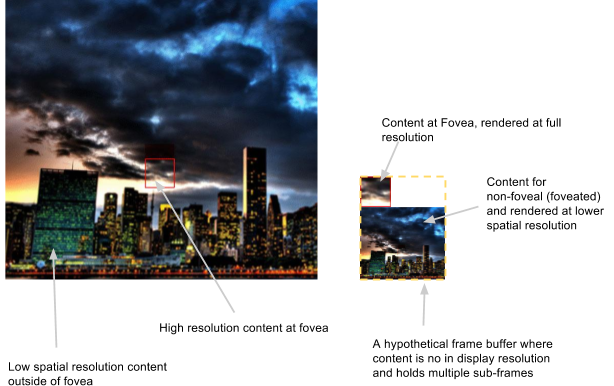
In the human visual system, the fovea centralis allows us to see at high-fidelity in the center of our vision, allowing our brain to pay less attention to things in our peripheral vision. Foveated rendering takes advantage of this characteristic to improve the performance of the rendering engine by reducing the spatial or bit-depth resolution of objects in our peripheral vision. To make this work, the location of the High Acuity (HA) region needs to be updated with eye-tracking to align with eye saccades, which preserves the perception of a constant high-resolution across the field of view. In contrast, systems with no eye-tracking may need to render a much larger HA region.
The left image is rendered at full resolution. The right image uses two layers of foveation — one rendered at high resolution (inside the yellow region) and one at lower resolution (outside).
A traditional foveation technique may divide a frame buffer into multiple spatial resolution regions. Aliasing introduced by rendering to lower spatial resolution may cause perceptible temporal artifacts when there is motion in the content due to head motion or animation. Below we show an example of temporal artifacts introduced by head rotation.
A smooth full rendering (image on the left). The image on the right shows temporal artifacts introduced by motion in foveated region.
In the following sections, we present two different methods we use aimed at reducing these artifacts: Phase-Aligned Foveated Rendering and Conformal Foveated Rendering. Each of these methods provide different benefits for visual quality during rendering and are useful under different conditions.

Phase-Aligned Rendering
Aliasing occurs in the Low-Acuity (LA) region during foveated rendering due to the subsampling of rendered content. In traditional foveated rendering discussed above, these aliasing artifacts flicker from frame to frame, since the display pixel grid moves across the virtual scene as the user moves their head. The motion of these pixels relative to the scene cause any existing aliasing artifacts to flicker, which is highly perceptible to the user, even in the periphery.

In Phase-Aligned rendering, we force the LA region frustums to be aligned rotationally to the world (e.g. always facing north, east, south, etc.), not the current frame's head-rotation. The aliasing artifacts are mostly invariant to head pose and therefore much less detectable. After upsampling, these regions are then reprojected onto the final display screen to compensate for the user's head rotation, which reduces temporal flicker. As with traditional foveation, we render the high-acuity region in a separate pass, and overlay it onto the merged image at the location of the fovea. The figure below compares traditional foveated rendering with phase-aligned rendering, both at the same level of foveation.
Temporal artifacts in non-world aligned foveated rendered content (left) and the phase-aligned method (right).
This method gives a major benefit to reducing the severity of visual artifacts during foveated rendering. Although phase-aligned rendering is more expensive to compute than traditional foveation under the same level of acuity reduction, we can still yield a net savings by pushing foveation to more aggressive levels that would otherwise have yielded too many artifacts.

Conformal Rendering
Another approach for foveated rendering is to render content in a space that matches the smoothly varying reduction in resolution of our visual acuity, based on a nonlinear mapping of the screen distance from the visual fixation point.

This method gives two main benefits. First, by more closely matching the visual fidelity fall-off of the human eye, we can reduce the total number of pixels computed compared to other foveation techniques. Second, by using a smooth fall-off in fidelity, we prevent the user from seeing a clear dividing line between High-Acuity and Low-Acuity, which is often one of the first artifacts that is noticed. These benefits allow for aggressive foveation to be used while preserving the same quality levels, yielding more savings.

We perform this method by warping the vertices of the virtual scene into non-linear space. This scene is then rasterized at a reduced resolution, then unwarped into linear space as a post-processing effect combined with lens distortion correction.
Comparison of traditional foveation (left) to conformal rendering (right), where content is rendered to a space matched to visual perception acuity and HMD lens characteristics. Both methods use the same number of total pixels.
A major benefit of this method over the phase-aligned method above is that conformal rendering only requires a single pass of rasterization. For scenes with lots of vertices, this difference can provide major savings. Additionally, although phase-aligned rendering reduces flicker, it still produces a distinct boundary between the high- and low-acuity regions, whereas conformal rendering does not show this artifact. However, a downside of conformal rendering compared to phase-alignment is that aliasing artifacts still flicker in the periphery, which may be less desirable for applications that require high visual fidelity.

Foveated Image Processing
HMDs often require image processing steps to be performed after rendering, such as local tone mapping, lens distortion correction, or lighting blending. With foveated image-processing, different operations are applied for different foveation regions. As an example, lens distortion correction, including chromatic aberration correction, may not require the same spatial accuracy for each part of the display. By running lens distortion correction on foveated content before upscaling, significant savings are gained in computation. This technique does not introduce perceptible artifacts.
Correction for head-mounted-display lens chromatic aberration in foveated space. Top image shows the conventional pipeline. The bottom image (in Green) shows the operation in the foveated space.
The left image shows reconstructed foveated content after lens distortion. The right image shows image difference when lens distortion correction is performed in a foveated manner. The right image shows that minimal error is introduced close to edges of frame buffer. These errors are imperceptible in an HMD.

Foveated Transmission
A non-trivial source of power consumption for standalone HMDs is data transmission from the system-on-a-chip (SoC) to the display module. Foveated transmission aims to save power and bandwidth by transmitting the minimum amount of data necessary to the display as shown in figure below.
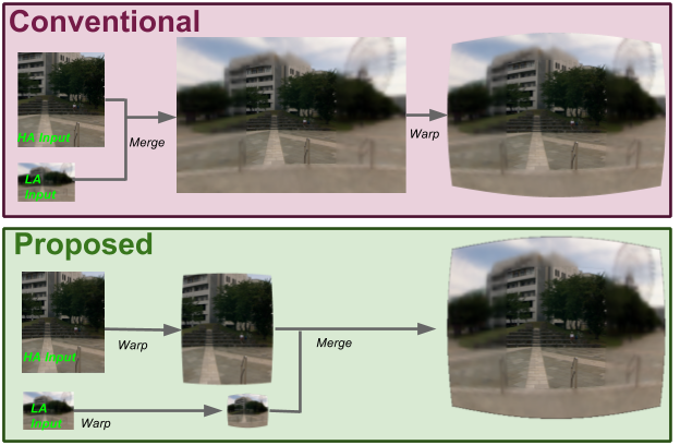
Rather than streaming upscaled foveated content (left image), foveated transmission enables streaming content pre-reconstruction (right image) and reducing the number of bits transmitted.
This change requires moving the simple upscaling and blending operations to the display side and transmitting only the foveated rendered content. Complexity arises if the foveal region, the red box in above figure, moves with eyetracking. Such motion may cause temporal artifacts (figure below) since Display Stream Compression (DSC) used between SoC and the display is not designed for foveated content.
Comparison of full integration of foveation and compression techniques (left) versus typical flickering artifacts that may be introduced by applying DSC to foveated content (right).
Toward a New Pipeline
We have focused on a few components of a “foveation pipeline” for MR and VR applications. By considering the impact of foveation in every part of a display system — rendering, processing and transmission — we can enable the next generation of lightweight, low-power, and high resolution MR/VR HMDs. This topic has been an active area of research for many years and it seems reasonable to expect the appearance of VR and MR headsets with foveated pipelines in the coming years.

Acknowledgements
We would like to recognize the work done by the following collaborators:
  • Haomiao Jiang and Carlin Vieri on display compression and foveated transmission
  • Brian Funt and Sylvain Vignaud on the development of new foveated rendering algorithms

Seamless Google Street View Panoramas


In 2007, we introduced Google Street View, enabling you to explore the world through panoramas of neighborhoods, landmarks, museums and more, right from your browser or mobile device. The creation of these panoramas is a complicated process, involving capturing images from a multi-camera rig called a rosette, and then using image blending techniques to carefully stitch them all together. However, many things can thwart the creation of a "successful" panorama, such as mis-calibration of the rosette camera geometry, timing differences between adjacent cameras, and parallax. And while we attempt to address these issues by using approximate scene geometry to account for parallax and frequent camera re-calibration, visible seams in image overlap regions can still occur.
Left: A Street View car carrying a multi-camera rosette. Center: A close-up of the rosette, which is made up of 15 cameras. Right: A visualization of the spatial coverage of each camera. Overlap between adjacent cameras is shown in darker gray.
Left: The Sydney Opera House with stitching seams along its iconic shells. Right: The same Street View panorama after optical flow seam repair.
In order to provide more seamless Street View images, we’ve developed a new algorithm based on optical flow to help solve these challenges. The idea is to subtly warp each input image such that the image content lines up within regions of overlap. This needs to be done carefully to avoid introducing new types of visual artifacts. The approach must also be robust to varying scene geometry, lighting conditions, calibration quality, and many other conditions. To simplify the task of aligning the images and to satisfy computational requirements, we’ve broken it into two steps.

Optical Flow
The first step is to find corresponding pixel locations for each pair of images that overlap. Using techniques described in our PhotoScan blog post, we compute optical flow from one image to the other. This provides a smooth and dense correspondence field. We then downsample the correspondences for computational efficiency. We also discard correspondences where there isn’t enough visual structure to be confident in the results of optical flow.

The boundaries of a pair of constituent images from the rosette camera rig that need to be stitched together.
An illustration of optical flow within the pair’s overlap region.
Extracted correspondences in the pair of images. For each colored dot in the overlap region of the left image, there is an equivalently-colored dot in the overlap region of the right image, indicating how the optical flow algorithm has aligned the point. These pairs of corresponding points are used as input to the global optimization stage. Notice that the overlap covers only a small portion of each image.
Global Optimization
The second step is to warp the rosette’s images to simultaneously align all of the corresponding points from overlap regions (as seen in the figure above). When stitched into a panorama, the set of warped images will then properly align. This is challenging because the overlap regions cover only a small fraction of each image, resulting in an under-constrained problem. To generate visually pleasing results across the whole image, we formulate the warping as a spline-based flow field with spatial regularization. The spline parameters are solved for in a non-linear optimization using Google’s open source Ceres Solver.
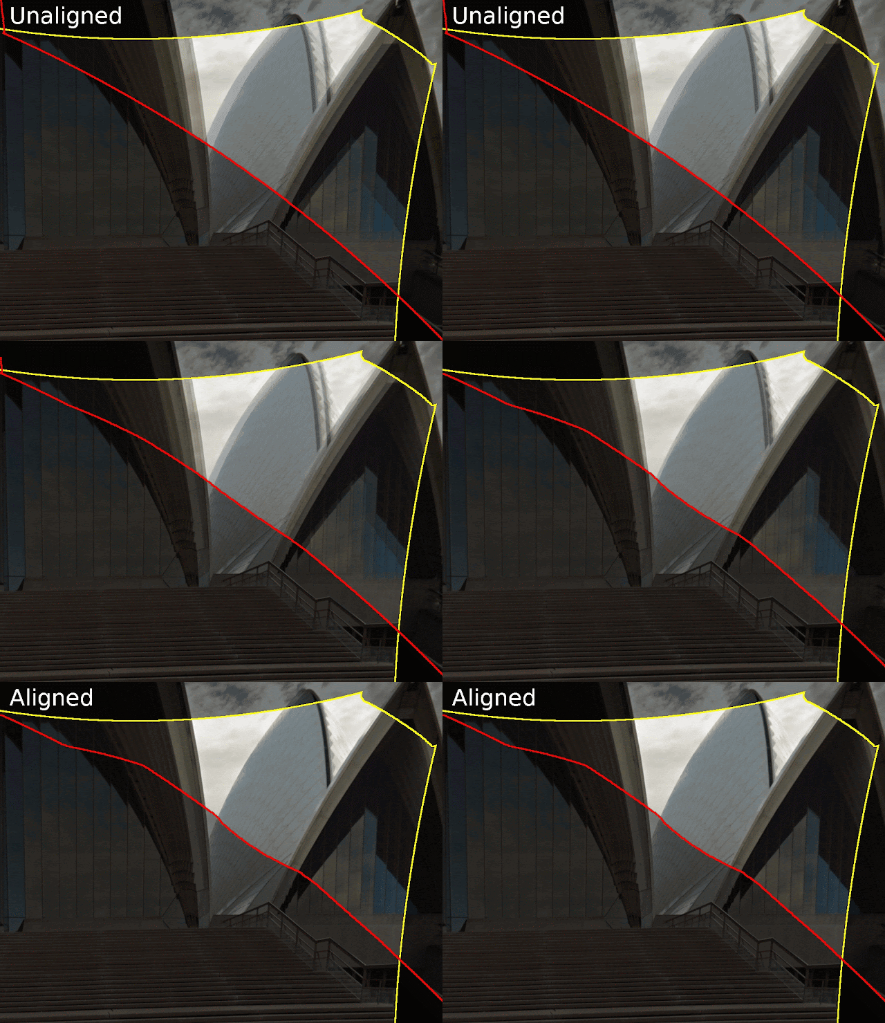
A visualization of the final warping process. Left: A section of the panorama covering 180 degrees horizontally. Notice that the overall effect of warping is intentionally quite subtle. Right: A close-up, highlighting how warping repairs the seams.
Our approach has many similarities to previously published work by Shum & Szeliski on “deghosting” panoramas. Key differences include that our approach estimates dense, smooth correspondences (rather than patch-wise, independent correspondences), and we solve a nonlinear optimization for the final warping. The result is a more well-behaved warping that is less likely to introduce new visual artifacts than the kernel-based approach.
Left: A close-up of the un-repaired panorama. Middle: Result of kernel-based interpolation. This fixes discontinuities but at the expense of strong wobbling artifacts due to the small image overlap and limited footprint of kernels. Right: Result of our global optimization.
This is important because our algorithm needs to be robust to the enormous diversity in content in Street View’s billions of panoramas. You can see how effective the algorithm is in the following examples:
Tower Bridge, London
Christ the Redeemer, Rio de Janeiro
An SUV on the streets of Seattle
This new algorithm was recently added to the Street View stitching pipeline. It is now being used to restitch existing panoramas on an ongoing basis. Keep an eye out for improved Street View near you!

Acknowledgements
Special thanks to Bryan Klingner for helping to integrate this feature with the Street View infrastructure.

Google at KDD’17: Graph Mining and Beyond


The 23rd ACM conference on Knowledge Discovery and Data Mining (KDD’17), a main venue for academic and industry research in data science, information retrieval, data mining and machine learning, was held last week in Halifax, Canada. Google has historically been an active participant in KDD, and this year was no exception, with Googlers’ contributing numerous papers and participating in workshops.

In addition to our overall participation, we are happy to congratulate fellow Googler Bryan Perozzi for receiving the SIGKDD 2017 Doctoral Dissertation Award, which serves to recognize excellent research by doctoral candidates in the field of data mining and knowledge discovery. This award was given in recognition of his thesis on the topic of machine learning on graphs performed at Stony Brook University, under the advisorship of Steven Skiena. Part of his thesis was developed during his internships at Google. The thesis dealt with using a restricted set of local graph primitives (such as ego-networks and truncated random walks) to effectively exploit the information around each vertex for classification, clustering, and anomaly detection. Most notably, the work introduced the random-walk paradigm for graph embedding with neural networks in DeepWalk.

DeepWalk: Online Learning of Social Representations, originally presented at KDD'14, outlines a method for using a series of local information obtained from truncated random walks to learn latent representations of nodes in a graph (e.g. users in a social network). The core idea was to treat each segment of a random walk as a sentence “in the language of the graph.” These segments could then be used as input for neural network models to learn representations of the graph’s nodes, using sequence modeling methods like word2vec (which had just been developed at the time). This research continues at Google, most recently with Learning Edge Representations via Low-Rank Asymmetric Projections.

The full list of Google contributions at KDD’17 is listed below (Googlers highlighted in blue).

Organizing Committee
Panel Chair: Andrew Tomkins
Research Track Program Chair: Ravi Kumar
Applied Data Science Track Program Chair: Roberto J. Bayardo
Research Track Program Committee: Sergei Vassilvitskii, Alex Beutel, Abhimanyu Das, Nan Du, Alessandro Epasto, Alex Fabrikant, Silvio Lattanzi, Kristen Lefevre, Bryan Perozzi, Karthik Raman, Steffen Rendle, Xiao Yu
Applied Data Science Program Track Committee: Edith Cohen, Ariel Fuxman, D. Sculley, Isabelle Stanton, Martin Zinkevich, Amr Ahmed, Azin Ashkan, Michael Bendersky, James Cook, Nan Du, Balaji Gopalan, Samuel Huston, Konstantinos Kollias, James Kunz, Liang Tang, Morteza Zadimoghaddam

Awards
Doctoral Dissertation Award: Bryan Perozzi, for Local Modeling of Attributed Graphs: Algorithms and Applications.

Doctoral Dissertation Runner-up Award: Alex Beutel, for User Behavior Modeling with Large-Scale Graph Analysis.

Papers
Ego-Splitting Framework: from Non-Overlapping to Overlapping Clusters
Alessandro Epasto, Silvio Lattanzi, Renato Paes Leme

HyperLogLog Hyperextended: Sketches for Concave Sublinear Frequency Statistics
Edith Cohen

Google Vizier: A Service for Black-Box Optimization
Daniel Golovin, Benjamin Solnik, Subhodeep Moitra, Greg Kochanski, John Karro, D. Sculley

Quick Access: Building a Smart Experience for Google Drive
Sandeep Tata, Alexandrin Popescul, Marc Najork, Mike Colagrosso, Julian Gibbons, Alan Green, Alexandre Mah, Michael Smith, Divanshu Garg, Cayden Meyer, Reuben KanPapers

TFX: A TensorFlow­ Based Production ­Scale Machine Learning Platform
Denis Baylor, Eric Breck, Heng-Tze Cheng, Noah Fiedel, Chuan Yu Foo, Zakaria Haque, Salem Haykal, Mustafa Ispir, Vihan Jain, Levent Koc, Chiu Yuen Koo, Lukasz Lew, Clemens MewaldAkshay Modi, Neoklis Polyzotis, Sukriti Ramesh, Sudip Roy, Steven Whang, Martin Wicke Jarek Wilkiewicz, Xin Zhang, Martin Zinkevich

Construction of Directed 2K Graphs
Balint Tillman, Athina Markopoulou, Carter T. Butts, Minas Gjoka

A Practical Algorithm for Solving the Incoherence Problem of Topic Models In Industrial Applications
Amr Ahmed, James Long, Dan Silva, Yuan Wang

Train and Distribute: Managing Simplicity vs. Flexibility in High-­Level Machine Learning Frameworks
Heng-Tze Cheng, Lichan Hong, Mustafa Ispir, Clemens Mewald, Zakaria Haque, Illia Polosukhin, Georgios Roumpos, D Sculley, Jamie Smith, David Soergel, Yuan Tang, Philip Tucker, Martin Wicke, Cassandra Xia, Jianwei Xie

Learning to Count Mosquitoes for the Sterile Insect Technique
Yaniv Ovadia, Yoni Halpern, Dilip Krishnan, Josh Livni, Daniel Newburger, Ryan Poplin, Tiantian Zha, D. Sculley

Workshops
13th International Workshop on Mining and Learning with Graphs
Keynote Speaker: Vahab Mirrokni - Distributed Graph Mining: Theory and Practice
Contributed talks include:
HARP: Hierarchical Representation Learning for Networks
Haochen Chen, Bryan Perozzi, Yifan Hu and Steven Skiena

Fairness, Accountability, and Transparency in Machine Learning
Contributed talks include:
Fair Clustering Through Fairlets
Flavio Chierichetti, Ravi Kumar, Silvio Lattanzi, Sergei Vassilvitskii
Data Decisions and Theoretical Implications when Adversarially Learning Fair Representations
Alex Beutel, Jilin Chen, Zhe Zhao, Ed H. Chi

Tutorial
TensorFlow
Rajat Monga, Martin Wicke, Daniel ‘Wolff’ Dobson, Joshua Gordon

Announcing the NYC Algorithms and Optimization Site


New York City is home to several Google algorithms research groups. We collaborate closely with the teams behind many Google products and work on a wide variety of algorithmic challenges, like optimizing infrastructure, protecting privacy, improving friend suggestions and much more.

Today, we’re excited to provide more insights into the research done in the Big Apple with the launch of the NYC Algorithms and Optimization Team page. The NYC Algorithms and Optimization Team comprises multiple overlapping research groups working on large-scale graph mining, large-scale optimization and market algorithms.

Large-scale Graph Mining
The Large-scale Graph Mining Group is tasked with building the most scalable library for graph algorithms and analysis and applying it to a multitude of Google products. We formalize data mining and machine learning challenges as graph algorithms problems and perform fundamental research in those fields leading to publications in top venues.

Our projects include:
  • Large-scale Similarity Ranking: Our research in pairwise similarity ranking has produced a number of innovative methods, which we have published in top venues such as WWW, ICML, and VLDB, e.g., improving friend suggestion using ego-networks and computing similarity rankings in large-scale multi-categorical bipartite graphs.
  • Balanced Partitioning: Balanced partitioning is often a crucial first step in solving large-scale graph optimization problems. As our paper shows, we are able to achieve a 15-25% reduction in cut size compared to state-of-the-art algorithms in the literature.
  • Clustering and Connected Components: We have state-of-the-art implementations of many different algorithms including hierarchical clustering, overlapping clustering, local clustering, spectral clustering, and connected components. Our methods are 10-30x faster than the best previously studied algorithms and can scale to graphs with trillions of edges.
  • Public-private Graph Computation: Our research on novel models of graph computation based on a personal view of private data preserves the privacy of each user.
Large-scale Optimization
The Large-scale Optimization Group’s mission is to develop large-scale optimization techniques and use them to improve the efficiency and robustness of infrastructure at Google. We apply techniques from areas such as combinatorial optimization, online algorithms, and control theory to make Google’s massive computational infrastructure do more with less. We combine online and offline optimizations to achieve such goals as increasing throughput, decreasing latency, minimizing resource contention, maximizing the efficacy of caches, and eliminating unnecessary work in distributed systems.

Our research is used in critical infrastructure that supports core products:
  • Consistent Hashing: We designed memoryless balanced allocation algorithms to assign a dynamic set of clients to a dynamic set of servers such that the load on each server is bounded, and the allocation does not change by much for every update operation. This technique is currently implemented in Google Cloud Pub/Sub and externally in the open-source haproxy.
  • Distributed Optimization Based on Core-sets: Composable core-sets provide an effective method for solving optimization problems on massive datasets. This technique can be used for several problems including distributed balanced clustering and distributed submodular maximization.
  • Google Search Infrastructure Optimization: We partnered with the Google Search infrastructure team to build a distributed feedback control loop to govern the way queries are fanned out to machines. We also improved the efficacy of caching by increasing the homogeneity of the stream of queries seen by any single machine.
Market Algorithms
The Market Algorithms Group analyzes, designs, and delivers economically and computationally efficient marketplaces across Google. Our research serves to optimize display ads for DoubleClick’s reservation ads and exchange, as well as sponsored search and mobile ads.

In the past few years, we have explored a number of areas, including:
For a summary of our research activities, you can take a look at talks at our recent market algorithms workshop.

It is our hope that with the help of this new Google NYC Algorithms and Optimization Team page that we can more effectively share our work and broaden our dialogue with the research and engineering community. Please visit the site to learn about our latest projects, publications, seminars, and research areas!

Consistent Hashing with Bounded Loads


Running a large-scale web service, such as content hosting, necessarily requires load balancing — distributing clients uniformly across multiple servers such that none get overloaded. Further, it is desirable to find an allocation that does not change very much over time in a dynamic environment in which both clients and servers can be added or removed at any time. In other words, we need the allocation of clients to servers to be consistent over time.

In collaboration with Mikkel Thorup, a visiting researcher from university of Copenhagen, we developed a new efficient allocation algorithm for this problem with tight guarantees on the maximum load of each server, and studied it theoretically and empirically. We then worked with our Cloud team to implement it in Google Cloud Pub/Sub, a scalable event streaming service, and observed substantial improvement on uniformity of the load allocation (in terms of the maximum load assigned to servers) while maintaining consistency and stability objectives. In August 2016 we described our algorithm in the paper “Consistent Hashing with Bounded Loads”, and shared it on ArXiv for potential use by the broader research community.

Three months later, Andrew Rodland from Vimeo informed us that he had found the paper, implemented it in haproxy (a widely-used piece of open source software), and used it for their load balancing project at Vimeo. The results were dramatic: applying these algorithmic ideas helped them decrease the cache bandwidth by a factor of almost 8, eliminating a scaling bottleneck. He recently summarized this story in a blog post detailing his use case. Needless to say, we were excited to learn that our theoretical research was not only put into application, but also that it was useful and open-sourced.

Background
While the concept of consistent hashing has been developed in the past to deal with load balancing in dynamic environments, a fundamental issue with all the previously developed schemes is that, in certain scenarios, they may result in sub-optimal load balancing on many servers.

Additionally, both clients and servers may be added or removed periodically, and with such changes, we do not want to move too many clients. Thus, while the dynamic allocation algorithm has to always ensure a proper load balancing, it should also aim to minimize the number of clients moved after each change to the system. Such allocation problems become even more challenging when we face hard constraints on the capacity of each server - that is, each server has a capacity that the load may not exceed. Typically, we want capacities close to the average loads.

In other words, we want to simultaneously achieve both uniformity and consistency in the resulting allocations. There is a vast amount of literature on solutions in the much simpler case where the set of servers is fixed and only the client set is updated, but in this post we discuss solutions that are relevant in the fully dynamic case where both clients and servers can be added and removed.

The Algorithm
We can think about the servers as bins and clients as balls to have a similar notation with well-studied balls-to-bins stochastic processes. The uniformity objective encourages all bins to have a load roughly equal to the average density (the number of balls divided by the number of bins). For some parameter ε, we set the capacity of each bin to either floor or ceiling of the average load times (1+ε). This extra capacity allows us to design an allocation algorithm that meets the consistency objective in addition to the uniformity property.

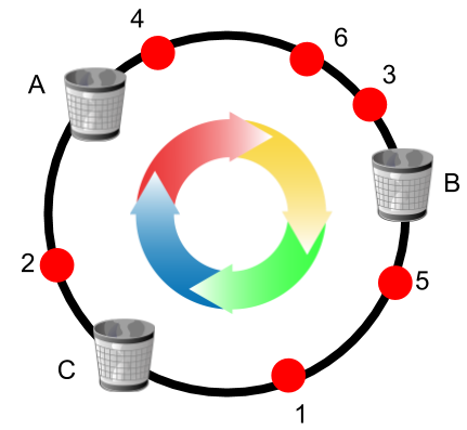
Imagine a given range of numbers overlaid on a circle. We apply a hash function to balls and a separate hash function to bins to obtain numbers in that range that correspond to positions on that circle. We then start allocating balls in a specific order independent of their hash values (let’s say based on their ID). Then each ball is moved clockwise and is assigned to the first bin with spare capacity.
Consider the example above where 6 balls and 3 bins are assigned using two separate hash functions to random locations on the circle. For the sake of this instance, assume the capacity of each bin is set to 2. We start allocating balls in the increasing order of their ID values. Ball number 1 moves clockwise, and goes to bin C. Ball number 2 goes to A. Balls 3 and 4 go to bin B. Ball number 5 goes to bin C. Then ball number 6 moves clockwise and hits bin B first. However bin B has capacity 2 and already contains balls 3 and 4. So ball 6 keeps moving to reach bin C but that bin is also full. Finally, ball 6 ends up in bin A that has a spare slot for it.

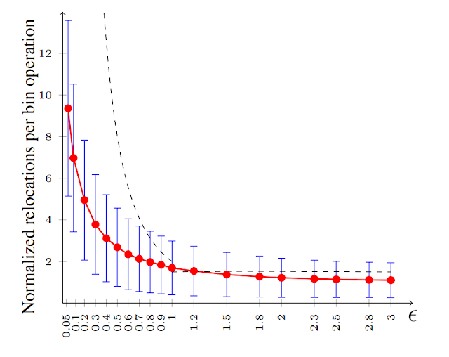
Upon any update in the system (ball or bin insertion/deletion), the allocation is recomputed to keep the uniformity objective. The art of the analysis is to show that a small update (a few number of insertions and deletions) results in minor changes in the state of the allocation and therefore the consistency objective is met. In our paper we show that every ball removal or insertion in the system results in O(1/ε2) movements of other balls. The most important thing about this upper bound is that it is independent of the total number of balls or bins in the system. So if the number of balls or bins are doubled, this bound will not change. Having an upper bound independent of the number of balls or bins introduces room for scalability as the consistency objective is not violated if we move to bigger instances. Simulations for the number of movements (relocations) per update is shown below when an update occurs on a bin/server.
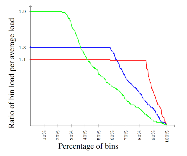
The red curve shows the average number of movements and the blue bars indicate the variance for different values of ε (the x-axis). The dashed curve is the upper bound suggested by our theoretical results which fits nicely as a prediction of the actual number of movements. Furthermore, for any value of ε, we know the load of each bin is at most (1+ε) times the average load. Below we see the load distribution of bins for different values of ε=0.1, ε=0.3 and ε=0.9.
The distribution of loads for several values of ε. The load distribution is nearly uniform covering all ranges of loads from 0 to (1+ε) times average, and many bins with load equal to (1+ε) times average.
As one can see there is a tradeoff — a lower ε helps with uniformity but not with consistency, while larger ε values help with consistency. A lower ε will ensure that many loads will be equal to the hard capacity limit of (1+ε) times the average, and the rest have a decaying distribution.

When providing content hosting services, one must be ready to face a variety of instances with different characteristics. This consistent hashing scheme is ideal for such scenarios as it performs well even for worst-case instances.

While our internal results are exciting, we are even more pleased that the broader community found our solution useful enough to open-source, allowing anyone to use this algorithm. If you are interested in further details of this research, please see the paper on ArXiv, and stay tuned for more research from the NYC Algorithms Team!

Acknowledgements:
We would like to thank Alex Totok, Matt Gruskin, Sergey Kondratyev and Haakon Ringberg from the Google Cloud Pub/Sub team, and of course Mikkel Thorup for his invaluable contributions to this paper.

The 280-Year-Old Algorithm Inside Google Trips


Algorithms Engineering is a lot of fun because algorithms do not go out of fashion: one never knows when an oldie-but-goodie might come in handy. Case in point: Yesterday, Google announced Google Trips, a new app to assist you in your travels by helping you create your own “perfect day” in a city. Surprisingly, deep inside Google Trips, there is an algorithm that was invented 280 years ago.

In 1736, Leonhard Euler authored a brief but beautiful mathematical paper regarding the town of Königsberg and its 7 bridges, shown here:
Image from Wikipedia
In the paper, Euler studied the following question: is it possible to walk through the city crossing each bridge exactly once? As it turns out, for the city of Königsberg, the answer is no. To reach this answer, Euler developed a general approach to represent any layout of landmasses and bridges in terms of what he dubbed the Geometriam Situs (the “Geometry of Place”), which we now call Graph Theory. He represented each landmass as a “node” in the graph, and each bridge as an “edge,” like this:
Image from Wikipedia
Euler noticed that if all the nodes in the graph have an even number of edges (such graphs are called “Eulerian” in his honor) then, and only then, a cycle can be found that visits every edge exactly once. Keep this in mind, as we’ll rely on this fact later in the post.

Our team in Google Research has been fascinated by the “Geometry of Place” for some time, and we started investigating a question related to Euler’s: rather than visiting just the bridges, how can we visit as many interesting places as possible during a particular trip? We call this the “itineraries” problem. Euler didn’t study it, but it is a well known topic in Optimization, where it is often called the “Orienteering” problem.

While Euler’s problem has an efficient and exact solution, the itineraries problem is not just hard to solve, it is hard to even approximately solve! The difficulty lies in the interplay between two conflicting goals: first, we should pick great places to visit, but second, we should pick them to allow a good itinerary: not too much travel time; don’t visit places when they’re closed; don’t visit too many museums, etc. Embedded in such problems is the challenge of finding efficient routes, often referred to as the Travelling Salesman Problem (TSP).

Algorithms for Travel Itineraries

Fortunately, the real world has a property called the “triangle inequality” that says adding an extra stop to a route never makes it shorter. When the underlying geometry satisfies the triangle inequality, the TSP can be approximately solved using another algorithm discovered by Christofides in 1976. This is an important part of our solution, and builds on Euler’s paper, so we’ll give a quick four-step rundown of how it works here:
  1. We start with all our destinations separate, and repeatedly connect together the closest two that aren’t yet connected. This doesn’t yet give us an itinerary, but it does connect all the destinations via a minimum spanning tree of the graph.
  2. We take all the destinations that have an odd number of connections in this tree (Euler proved there must be an even number of these), and carefully pair them up.
  3. Because all the destinations now have an even number of edges, we’ve created an Eulerian graph, so we create a route that crosses each edge exactly once.
  4. We now have a great route, but it might visit some places more than once. No problem, we find any double visits and simply bypass them, going directly from the predecessor to the successor.
Christofides gave an elegant proof that the resulting route is always close to the shortest possible. Here’s an example of the Christofides’ algorithm in action on a location graph with the nodes representing places and the edges with costs representing the travel time between the places.
Construction of an Eulerian Tour in a location graph
Armed with this efficient route-finding subroutine, we can now start building itineraries one step at a time. At each step, we estimate the benefit to the user of each possible new place to visit, and likewise estimate the cost using the Christofides algorithm. A user’s benefit can be derived from a host of natural factors such as the popularity of the place and how different the place is relative to places already visited on the tour. We then pick whichever new place has the best benefit per unit of extra cost (e.g., time needed to include the new place in the tour). Here’s an example of our algorithm actually building a route in London using the location graph shown above:
Itineraries in Google Trips

With our first good approximate solution to the itineraries problem in hand, we started working with our colleagues from the Google Trips team, and we realized we’d barely scratched the surface. For instance, even if we produce the absolute perfect itinerary, any particular user of the system will very reasonably say, “That’s great, but all my friends say I also need to visit this other place. Plus, I’m only around for the morning, and I don’t want to miss this place you listed in the afternoon. And I’ve already seen Big Ben twice.” So rather than just producing an itinerary once and calling it a perfect day, we needed a fast dynamic algorithm for itineraries that users can modify on the fly to suit their individual taste. And because many people have bad data connections while traveling, the solution had to be efficient enough to run disconnected on a phone.

Better Itineraries Through the Wisdom of Crowds

While the algorithmic aspects of the problem were highly challenging, we realized that producing high-quality itineraries was just as dependent on our understanding of the many possible stopping points on the itinerary. We had Google’s extensive travel database to identify the interesting places to visit, and we also had great data from Google’s existing systems about how to travel from any place to any other. But we didn’t have a good sense for how people typically move through this geometry of places.

For this, we turned to the wisdom of crowds. This type of wisdom is used by Google to estimate delays on highways, and to discover when restaurants are most busy. Here, we use the same techniques to learn about common visit sequences that we can stitch together into itineraries that feel good to our users. We combine Google's knowledge of when places are popular, with the directions between those places to gather an idea of what tourists like to do when travelling.

And the crowd has a lot more wisdom to offer in the future. For example, we noticed that visits to Buckingham Palace spike around 11:30 and stay a bit longer than at other times of the day. This seemed a little strange to us, but when we looked more closely, it turns out to be the time of the Changing of the Guard. We’re looking now at ways to incorporate this type of timing information into the itinerary selection algorithms.

So give it a try: Google Trips, available now on Android and iOS, has you covered from departure to return.

Research from VLDB 2016: Improved Friend Suggestion using Ego-Net Analysis


On September 5 - 9, New Delhi, India hosted the 42nd International Conference on Very Large Data Bases (VLDB), a premier annual forum for academic and industry research on databases, data management, data mining and data analytics. Over the past several years, Google has actively participated in VLDB, both as official sponsor and with numerous contributions to the research and industrial tracks. In this post, we would like to share the research presented in one of the Google papers from VLDB 2016.

In Ego-net Community Mining Applied to Friend Suggestion, co-authored by Googlers Silvio Lattanzi, Vahab Mirrokni, Ismail Oner Sebe, Ahmed Taei, Sunita Verma and myself, we explore how social networks can provide better friend suggestions to users, a challenging practical problem faced by all social network platforms

Friend suggestion – the task of suggesting to a user the contacts she might already know in the network but that she hasn’t added yet – is major driver of user engagement and social connection in all online social networks. Designing a high quality system that can provide relevant and useful friend recommendations is very challenging, and requires state-of-the-art machine learning algorithms based on a multitude of parameters.

An effective family of features for friend suggestion consist of graph features such as the number of common friends between two users. While widely used, the number of common friends has some major drawbacks, including the following which is shown in Figure 1.
Figure 1: Ego-net of Sally.
In this figure we represent the social connections of Sally and her friends – the ego-net of Sally. An ego-net of a node (in this case, Sally) is defined as the graph that contains the node itself, all of the node’s neighbors and the connection among those nodes. Sally has 6 friends in her ego-net: Albert (her husband), Brian (her son), Charlotte (her mother) as well as Uma (her boss), Vincent and Wally (two of her team members). Notice how A, B and C are all connected with each other while they do not know U, V or W. On the other hand U, V and W have all added each other as their friend (except U and W who are good friend but somehow forgot to add each other).

Notice how each of A, B, C have a common friend with each of U, V and W: Sally herself. A friend recommendation system based on common neighbors might suggest to Sally’s son (for instance) to add Sally’s boss as his friend! In reality the situation is even more complicated because users’ online and offline friends span several different social circles or communities (family, work, school, sports, etc).

In our paper we introduce a novel technique for friend suggestions based on independently analyzing the ego-net structure. The main contribution of the paper is to show that it is possible to provide friend suggestions efficiently by constructing all ego-nets of the nodes in the graph and then independently applying community detection algorithms on them in large-scale distributed systems.

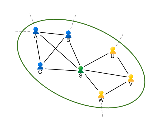
Specifically, the algorithm proceeds by constructing the ego-nets of all nodes and applying, independently on each of them, a community detection algorithm. More precisely the algorithm operates on so-called “ego-net-minus-ego” graphs, which is defined as the graph including only the neighbors of a given node, as shown in the figure below.
Figure 2: Clustering of the ego-net of Sally.
Notice how in this example the ego-net-minus-ego of Sally has two very clear communities: her family (A, B, C) and her co-workers (U, V, W) which are easily separated. Intuitively, this is because one might expect that while nodes (e.g. Sally) participate in many communities, there is usually a single (or a limited number of) contexts in which two specific neighbors interact. While Sally is both part of her family and work community, Sally and Uma interact only at work. Through extensive experimental evaluation on large-scale public social networks and formally through a simple mathematical model, our paper confirms this intuition. It seems that while communities are hard to separate in a global graph, they are easier to identify at the local level of ego-nets.

This allows for a novel graph-based method for friend suggestion which intuitively only allows suggestion of pairs of users that are clustered together in the same community from the point of view of their common friends. With this method, U and W will be suggested to add each other (as they are in the same community and they are not yet connected) while B and U will not be suggested as friends as they span two different communities.

From an algorithmic point of view, the paper introduces efficient parallel and distributed techniques for computing and clustering all ego-nets of very large graphs at the same time – a fundamental aspect enabling use of the system on the entire world Google+ graph. We have applied this feature in the “You May Know” system of Google+, resulting in a clear positive impact on the prediction task, improving the acceptance rate by more than 1.5% and decreasing the rejection rate by more than 3.3% (a significative impact at Google scales).

We believe that many future directions of work might stem from our preliminary results. For instance ego-net analysis could be potentially to automatically classify a user contacts in circles and to detect spam. Another interesting direction is the study of ego-network evolution in dynamic graphs.