Tag Archives: algorithms

Robust Online Allocation with Dual Mirror Descent

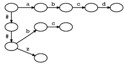
The emergence of digital technologies has transformed decision making across commercial sectors such as airlines, online retailing, and internet advertising. Today, real-time decisions need to be repeatedly made in highly uncertain and rapidly changing environments. Moreover, organizations usually have limited resources, which need to be efficiently allocated across decisions. Such problems are referred to as online allocation problems with resource constraints, and applications abound. Some examples include:

  • Bidding with Budget Constraints: Advertisers increasingly purchase ad slots using auction-based marketplaces such as search engines and ad exchanges. A typical advertiser can participate in a large number of auctions in a given month. Because the supply in these marketplaces is uncertain, advertisers set budgets to control their total spend. Therefore, advertisers need to determine how to optimally place bids while limiting total spend and maximizing conversions.
  • Dynamic Ad Allocation: Publishers can monetize their websites by signing deals with advertisers guaranteeing a number of impressions or by auctioning off slots in the open market. To make this choice, publishers need to trade off, in real-time, the short-term revenue from selling slots in the open market and the long-term benefits of delivering good quality spots to reservation ads.
  • Airline Revenue Management: Planes have a limited number of seats that need to be filled up as much as possible before a flight’s departure. But demand for flights changes over time and airlines would like to sell airline tickets to the customers who are willing to pay the most. Thus, airlines have increasingly adopted sophisticated automated systems to manage the pricing and availability of airline tickets.
  • Personalized Retailing with Limited Inventories: Online retailers can use real-time data to personalize their offerings to customers who visit their store. Because product inventory is limited and cannot be easily replenished, retailers need to dynamically decide which products to offer and at what price to maximize their revenue while satisfying their inventory constraints.

The common feature of these problems is the presence of resource constraints (budgets, contractual obligations, seats, or inventory, respectively in the examples above) and the need to make dynamic decisions in environments with uncertainty. Resource constraints are challenging because they link decisions across time — e.g., in the bidding problem, bidding too high early can leave advertisers with no budget, and thus missed opportunities later. Conversely, bidding too conservatively can result in a low number of conversions or clicks.

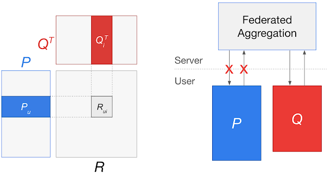
Two central resource allocation problems faced by advertisers and publishers in internet advertising markets.

In this post, we discuss state-of-the-art algorithms that can help maximize goals in dynamic, resource-constrained environments. In particular, we have recently developed a new class of algorithms for online allocation problems, called dual mirror descent, that are simple, robust, and flexible. Our papers have appeared in Operations Research, ICML’20, and ICML’21, and we have ongoing work to continue progress in this space. Compared to existing approaches, dual mirror descent is faster as it does not require solving auxiliary optimization problems, is more flexible because it can handle many applications across different sectors with minimal modifications, and is more robust as it enjoys remarkable performance under different environments.

Online Allocation Problems
In an online allocation problem, a decision maker has a limited amount of total resources (B) and receives a certain number of requests over time (T). At any point in time (t), the decision maker receives a reward function (ft) and resource consumption function (bt), and takes an action (xt). The reward and resource consumption functions change over time and the objective is to maximize the total reward within the resource constraints. If all the requests were known in advance, then an optimal allocation could be obtained by solving an offline optimization problem for how to maximize the reward function over time within the resource constraints1.

The optimal offline allocation cannot be implemented in practice because it requires knowing future requests. However, this is still useful for framing the goal of online allocation problems: to design an algorithm whose performance is as close to optimal as possible without knowing future requests.

Achieving the Best of Many Worlds with Dual Mirror Descent
A simple, yet powerful idea to handle resource constraints is introducing “prices” for the resources, which enables accounting for the opportunity cost of consuming resources when making decisions. For example, selling a seat on a plane today means it can’t be sold tomorrow. These prices are useful as an internal accounting system of the algorithm. They serve the purpose of coordinating decisions at different moments in time and allow decomposing a complex problem with resource constraints into simpler subproblems: one per time period with no resource constraints. For example, in a bidding problem, the prices capture an advertiser’s opportunity cost of consuming one unit of budget and allow the advertiser to handle each auction as an independent bidding problem.

This reframes the online allocation problem as a problem of pricing resources to enable optimal decision making. The key innovation of our algorithm is using machine learning to predict optimal prices in an online fashion: we choose prices dynamically using mirror descent, a popular optimization algorithm for training machine learning predictive models. Because prices for resources are referred to as "dual variables" in the field of optimization, we call the resulting algorithm dual mirror descent.

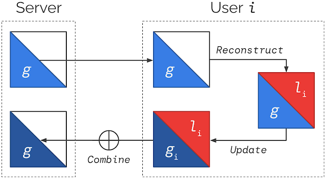
The algorithm works sequentially by assuming uniform resource consumption over time is optimal and updating the dual variables after each action. It starts at a moment in time (t) by taking an action (xt) that maximizes the reward minus the opportunity cost of consuming resources (shown in the top gray box below). The action (e.g., how much to bid or which ad to show) is implemented if there are enough resources available. Then, the algorithm computes the error in the resource consumption (gt), which is the difference between uniform consumption over time and the actual resource consumption (below in the third gray box). A new dual variable for the next time period is computed using mirror descent based on the error, which then informs the next action. Mirror descent seeks to make the error as close as possible to zero, improving the accuracy of its estimate of the dual variable, so that resources are consumed uniformly over time. While the assumption of uniform resource consumption may be surprising, it helps avoid missing good opportunities and often aligns with commercial goals so is effective. Mirror descent also allows a variety of update rules; more details are in the paper.

An overview of the dual mirror descent algorithm.

By design, dual mirror descent has a self-correcting feature that prevents depleting resources too early or waiting too long to consume resources and missing good opportunities. When a request consumes more or less resources than the target, the corresponding dual variable is increased or decreased. When resources are then priced higher or lower, future actions are chosen to consume resources more conservatively or aggressively.

This algorithm is easy to implement, fast, and enjoys remarkable performance under different environments. These are some salient features of our algorithm:

  • Existing methods require periodically solving large auxiliary optimization problems using past data. In contrast, this algorithm does not need to solve any auxiliary optimization problem and has a very simple rule to update the dual variables, which, in many cases, can be run in linear time complexity. Thus, it is appealing for many real-time applications that require fast decisions.
  • There are minimal requirements on the structure of the problem. Such flexibility allows dual mirror descent to handle many applications across different sectors with minimal modifications. Moreover, our algorithms are flexible since they accommodate different objectives, constraints, or regularizers. By incorporating regularizers, decision makers can include important objectives beyond economic efficiency, such as fairness.
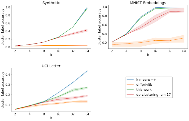
  • Existing algorithms for online allocation problems are tailored for either adversarial or stochastic input data. Algorithms for adversarial inputs are robust as they make almost no assumptions on the structure of the data but, in turn, obtain performance guarantees that are too pessimistic in practice. On the other hand, algorithms for stochastic inputs enjoy better performance guarantees by exploiting statistical patterns in the data but can perform poorly when the model is misspecified. Dual mirror descent, however, attains performance close to optimal in both stochastic and adversarial input models while being oblivious to the structure of the input model. Compared to existing work on simultaneous approximation algorithms, our method is more general, applies to a wide range of problems, and requires no forecasts. Below is a comparison of our algorithm to other state-of-the-art methods. Results are based on synthetic data for an ad allocation problem.
Performance of dual mirror descent, a training based method, and an adversarial method relative to the optimal offline solution. Lower values indicate performance closer to the optimal offline allocation. Results are generated using synthetic experiments based on public data for an ad allocation problem.

Conclusion
In this post we introduced dual mirror descent, an algorithm for online allocation problems that is simple, robust, and flexible. It is particularly notable that after a long line of work in online allocation algorithms, dual mirror descent provides a way to analyze a wider range of algorithms with superior robustness priorities compared to previous techniques. Dual mirror descent has a wide range of applications across several commercial sectors and has been used over time at Google to help advertisers capture more value through better algorithmic decision making. We are also exploring further work related to mirror descent and its connections to PI controllers.

Acknowledgements
We would like to thank our co-authors Haihao Lu and Balu Sivan, and Kshipra Bhawalkar for their exceptional support and contributions. We would also like to thank our collaborators in the ad quality team and market algorithm research.


1Formalized in the equation below: 

Source: Google AI Blog


Deep Learning with Label Differential Privacy

Over the last several years, there has been an increased focus on developing differential privacy (DP) machine learning (ML) algorithms. DP has been the basis of several practical deployments in industry — and has even been employed by the U.S. Census — because it enables the understanding of system and algorithm privacy guarantees. The underlying assumption of DP is that changing a single user’s contribution to an algorithm should not significantly change its output distribution.

In the standard supervised learning setting, a model is trained to make a prediction of the label for each input given a training set of example pairs {[input1,label1], …, [inputn, labeln]}. In the case of deep learning, previous work introduced a DP training framework, DP-SGD, that was integrated into TensorFlow and PyTorch. DP-SGD protects the privacy of each example pair [input, label] by adding noise to the stochastic gradient descent (SGD) training algorithm. Yet despite extensive efforts, in most cases, the accuracy of models trained with DP-SGD remains significantly lower than that of non-private models.

DP algorithms include a privacy budget, ε, which quantifies the worst-case privacy loss for each user. Specifically, ε reflects how much the probability of any particular output of a DP algorithm can change if one replaces any example of the training set with an arbitrarily different one. So, a smaller ε corresponds to better privacy, as the algorithm is more indifferent to changes of a single example. However, since smaller ε tends to hurt model utility more, it is not uncommon to consider ε up to 8 in deep learning applications. Notably, for the widely used multiclass image classification dataset, CIFAR-10, the highest reported accuracy (without pre-training) for DP models with ε = 3 is 69.3%, a result that relies on handcrafted visual features. In contrast, non-private scenarios (ε = ∞) with learned features have shown to achieve >95% accuracy while using modern neural network architectures. This performance gap remains a roadblock for many real-world applications to adopt DP. Moreover, despite recent advances, DP-SGD often comes with increased computation and memory overhead due to slower convergence and the need to compute the norm of the per-example gradient.

In “Deep Learning with Label Differential Privacy”, presented at NeurIPS 2021, we consider a more relaxed, but important, special case called label differential privacy (LabelDP), where we assume the inputs (input1, …, inputn) are public, and only the privacy of the training labels (label1, …, labeln) needs to be protected. With this relaxed guarantee, we can design novel algorithms that utilize a prior understanding of the labels to improve the model utility. We demonstrate that LabelDP achieves 20% higher accuracy than DP-SGD on the CIFAR-10 dataset. Our results across multiple tasks confirm that LabelDP could significantly narrow the performance gap between private models and their non-private counterparts, mitigating the challenges in real world applications. We also present a multi-stage algorithm for training deep neural networks with LabelDP. Finally, we are excited to release the code for this multi-stage training algorithm.

LabelDP
The notion of LabelDP has been studied in the Probably Approximately Correct (PAC) learning setting, and captures several practical scenarios. Examples include: (i) computational advertising, where impressions are known to the advertiser and thus considered non-sensitive, but conversions reveal user interest and are thus private; (ii) recommendation systems, where the choices are known to a streaming service provider, but the user ratings are considered sensitive; and (iii) user surveys and analytics, where demographic information (e.g., age, gender) is non-sensitive, but income is sensitive.

We make several key observations in this scenario. (i) When only the labels need to be protected, much simpler algorithms can be applied for data preprocessing to achieve LabelDP without any modifications to the existing deep learning training pipeline. For example, the classic Randomized Response (RR) algorithm, designed to eliminate evasive answer biases in survey aggregation, achieves LabelDP by simply flipping the label to a random one with a probability that depends on ε. (ii) Conditioned on the (public) input, we can compute a prior probability distribution, which provides a prior belief of the likelihood of the class labels for the given input. With a novel variant of RR, RR-with-prior, we can incorporate prior information to reduce the label noise while maintaining the same privacy guarantee as classical RR.

The figure below illustrates how RR-with-prior works. Assume a model is built to classify an input image into 10 categories. Consider a training example with the label “airplane”. To guarantee LabelDP, classical RR returns a random label sampled according to a given distribution (see the top-right panel of the figure below). The smaller the targeted privacy budget ε is, the larger the probability of sampling an incorrect label has to be. Now assume we have a prior probability showing that the given input is “likely an object that flies” (lower left panel). With the prior, RR-with-prior will discard all labels with small prior and only sample from the remaining labels. By dropping these unlikely labels, the probability of returning the correct label is significantly increased, while maintaining the same privacy budget ε (lower right panel).

Randomized response: If no prior information is given (top-left), all classes are sampled with equal probability. The probability of sampling the true class (P[airplane] ≈ 0.5) is higher if the privacy budget is higher (top-right). RR-with-prior: Assuming a prior distribution (bottom-left), unlikely classes are “suppressed” from the sampling distribution (bottom-right). So the probability of sampling the true class (P[airplane] ≈ 0.9) is increased under the same privacy budget.

A Multi-stage Training Algorithm
Based on the RR-with-prior observations, we present a multi-stage algorithm for training deep neural networks with LabelDP. First, the training set is randomly partitioned into multiple subsets. An initial model is then trained on the first subset using classical RR. Finally, the algorithm divides the data into multiple parts, and at each stage, a single part is used to train the model. The labels are produced using RR-with-prior, and the priors are based on the prediction of the model trained so far.

An illustration of the multi-stage training algorithm. The training set is partitioned into t disjoint subsets. An initial model is trained on the first subset using classical RR. Then the trained model is used to provide prior predictions in the RR-with-prior step and in the training of the later stages.

Results
We benchmark the multi-stage training algorithm’s empirical performance on multiple datasets, domains, and architectures. On the CIFAR-10 multi-class classification task for the same privacy budget ε, the multi-stage training algorithm (blue in the figure below) guaranteeing LabelDP achieves 20% higher accuracy than DP-SGD. We emphasize that LabelDP protects only the labels while DP-SGD protects both the inputs and labels, so this is not a strictly fair comparison. Nonetheless, this result demonstrates that for specific application scenarios where only the labels need to be protected, LabelDP could lead to significant improvements in the model utility while narrowing the performance gap between private models and public baselines.

Comparison of the model utility (test accuracy) of different algorithms under different privacy budgets.

In some domains, prior knowledge is naturally available or can be built using publicly available data only. For example, many machine learning systems have historical models which could be evaluated on new data to provide label priors. In domains where unsupervised or self-supervised learning algorithms work well, priors could also be built from models pre-trained on unlabeled (therefore public with respect to LabelDP) data. Specifically, we demonstrate two self-supervised learning algorithms in our CIFAR-10 evaluation (orange and green traces in the figure above). We use self-supervised learning models to compute representations for the training examples and run k-means clustering on the representations. Then, we spend a small amount of privacy budget (ε ≤ 0.05) to query a histogram of the label distribution of each cluster and use that as the label prior for the points in each cluster. This prior significantly boosts the model utility in the low privacy budget regime (ε < 1).

Similar observations hold across multiple datasets such as MNIST, Fashion-MNIST and non-vision domains, such as the MovieLens-1M movie rating task. Please see our paper for the full report on the empirical results.

The empirical results suggest that protecting the privacy of the labels can be significantly easier than protecting the privacy of both the inputs and labels. This can also be mathematically proven under specific settings. In particular, we can show that for convex stochastic optimization, the sample complexity of algorithms privatizing the labels is much smaller than that of algorithms privatizing both labels and inputs. In other words, to achieve the same level of model utility under the same privacy budget, LabelDP requires fewer training examples.

Conclusion
We demonstrated that both empirical and theoretical results suggest that LabelDP is a promising relaxation of the full DP guarantee. In applications where the privacy of the inputs does not need to be protected, LabelDP could reduce the performance gap between a private model and the non-private baseline. For future work, we plan to design better LabelDP algorithms for other tasks beyond multi-class classification. We hope that the release of the multi-stage training algorithm code provides researchers with a useful resource for DP research.

Acknowledgements
This work was carried out in collaboration with Badih Ghazi, Noah Golowich, and Ravi Kumar. We also thank Sami Torbey for valuable feedback on our work.

Source: Google AI Blog


Optimizing Airline Tail Assignments for Cleaner Skies

Airlines around the world are exploring several tactics to meet aggressive CO2 commitments set by the International Civil Aviation Organization (ICAO). This effort has been emphasized in Europe, where aviation accounts for 13.9% of the transportation industry’s carbon emissions. The largest push comes from the European Green Deal, which aims to decrease carbon emissions from transportation by 90% by 2051. The Lufthansa Group has gone even further, committing to a 50% reduction in emissions compared to 2019 by the year 2030 and to reach net-zero emissions by 2050.

One unexpected approach that airlines can use to lower carbon emissions is through optimizing their tail assignment, i.e., how to assign aircraft (identified by the aircraft registration painted on their tails) to legs in a way that minimizes the total operating cost, of which fuel is a major contributor. More fuel needed to operate the aircraft means higher operating costs and more carbon ejected into the atmosphere. For example, a typical long-haul flight (longer than ~4,100km or ~2,500mi) emits about a ton of CO2.

The amount of fuel needed to fly between origin and destination can vary widely — e.g., larger aircraft weigh more and therefore require more fuel, while modern and younger aircraft tend to be more fuel-efficient because they use newer technology. The mass of the fuel itself is also significant. Aircraft are less fuel-efficient early in their flights when their fuel tanks are full than later when the volume of fuel is reduced. Another important factor for the tail assignment is the number of passengers on board; as the number of bookings changes, a smaller or larger aircraft might be required. Other factors can affect fuel consumption, both negative (e.g., headwinds or the age of the engines) or positive (e.g., tailwinds, sharklets, skin).

During the past year, Google’s Operations Research team has been working with the Lufthansa Group to optimize their tail assignment to reduce carbon emissions and the cost of operating their flights. As part of this collaboration, we developed and launched a mathematical tail assignment solver that has been fully integrated to optimize the fleet schedule for SWISS International Air Lines (a Lufthansa Group subsidiary), which we estimate will result in significant reductions in carbon emissions. This solver is the first step of a multi-phase project that started at SWISS.

A Mathematical Model for Tail Assignment
We structure the task of tail assignment optimization as a network flow problem, which is essentially a directed graph characterized by a set of nodes and a set of arcs, with additional constraints related to the problem at hand. Nodes may have either a supply or a demand for a commodity, while arcs have a flow capacity and a cost per unit of flow. The goal is to determine flows for every arc that minimize the total flow cost of each commodity, while maintaining flow balance in the network.

We decided to use a flow network because it is the most common way of modeling this problem in literature, and the commodities, arcs, and nodes of the flow network have a simple one-to-one correspondence to tails, legs, and airports in the real-life problem. In this case, the arcs of the network correspond to each leg of the flight schedule, and each individual tail is a single instance of a commodity that “flows” along the network. Each leg and tail pair in the network has an associated assignment cost, and the model’s objective is to pick valid leg and tail pairs such that these assignment costs are minimized.

A simple example of the tail assignment problem. There are four legs in this schedule and four possible tails that one can assign to those legs. Each tail and leg pair has an associated operational cost. For example, for Leg 1, it costs $50 to assign Tail 1 to it but $100 to assign Tail 2. The optimal solution, with the minimum cost, is to assign Tail 4 to Legs 3 and 2 and Tail 1 to Legs 1 and 4.

Aside from the standard network flow constraints, the model takes into account additional airline-specific constraints so that the solution is tailored to Lufthansa Group airlines. For example, aircraft turnaround times — i.e., the amount of time an aircraft spends on the ground between two consecutive flights — are airline-specific and can vary for a number of reasons. Catering might be loaded at an airline's hub, reducing the turnaround time needed at outstations, or a route could have a higher volume of vacation travelers who often take longer to board and disembark than business travelers. Another constraint is that each aircraft must be on the ground for a nightly check at a specified airport’s maintenance hub to receive mandated maintenance work or cleaning. Furthermore, each airline has their own maintenance schedule, which can require aircraft to undergo routine maintenance checks every few nights, in part to help maintain the aircraft’s fuel efficiency.

Preliminary Results & Next Steps
After using our solver to optimize their fleet schedule in Europe, SWISS Airlines estimates an annual savings of over 3.5 million Swiss Francs and a 6500 ton reduction in CO2 emitted. We expect these savings will multiply when the model is rolled out to the rest of the airlines in the Lufthansa Group and again when traffic returns to pre-COVID levels. Future work will include ensuring this model is usable with larger sets of data, and adding crew and passenger assignment to the optimization system to improve the flight schedules for both passengers and flight crew.

If you are interested in experimenting with your own network flow models, check out OR-Tools, our open source software suite that can be used to build optimization solutions similar to the solver presented in this post. Refer to OR-Tools related documentation for more information.

Acknowledgements
Thanks to Jon Orwant for collaborating extensively on this blog post and for establishing the partnership with Lufthansa and SWISS, along with Alejandra Estanislao. Thanks to the Operations Research Team and to the folks at SWISS, this work could not be possible without their hard work and contributions.

Source: Google AI Blog


Robust Routing Using Electrical Flows

In the world of networks, there are models that can explain observations across a diverse collection of applications. These include simple tasks such as computing the shortest path, which has obvious applications to routing networks but also in biology, where the slime mold Physarum is able to find shortest paths in mazes. Another example is Braess’s paradox — the observation that adding resources to a network can have an effect opposite to the one expected — which manifests not only in road networks but also in mechanical and electrical systems, which can also be modeled as networks. For instance, constructing a new road can increase traffic congestion or adding a new link in an electrical circuit can increase voltage. Such connections between electrical circuits and other types of networks have been exploited for various tasks, such as partitioning networks, and routing flows.

In “Robust Routing Using Electrical Flows”, which won the Best Paper Award at SIGSPATIAL 2021, we present another interesting application of electrical flows in the context of road network routing. Specifically, we utilize ideas from electrical flows for the problem of constructing multiple alternate routes between a given source and destination. Alternate routes are important for many use cases, including finding routes that best match user preferences and for robust routing, e.g., routing that guarantees finding a good path in the presence of traffic jams. Along the way, we also describe how to quickly model electrical flows on road networks.

Existing Approaches to Alternate Routing
Computing alternate routes on road networks is a relatively new area of research and most techniques rely on one of two main templates: the penalty method and the plateau method. In the former, alternate routes are iteratively computed by running a shortest path algorithm and then, in subsequent runs, adding a penalty to those segments already included in the shortest paths that have been computed, to encourage further exploration. In the latter, two shortest path trees are built simultaneously, one starting from the origin and one from the destination, which are used to identify sequences of road segments that are common to both trees. Each such common sequence (which are expected to be important arterial streets for example) is then treated as a visit point on the way from the origin to the destination, thus potentially producing an alternate route. The penalty method is known to produce results of high quality (i.e., average travel time, diversity and robustness of the returned set of alternate routes) but is very slow in practice, whereas the plateau method is much faster but results in lower quality solutions.

An Alternate to Alternate Routing: Electrical Flows
Our approach is different and assumes that a routing problem on a road network is in many ways analogous to the flow of electrical current through a resistor network. Though the electrical current travels through many different paths, it is weaker along paths of higher resistance and stronger on low resistance ones, all else being equal.

We view the road network as a graph, where intersections are nodes and roads are edges. Our method then models the graph as an electrical circuit by replacing the edges with resistors, whose resistances equal the road traversal time, and then connecting a battery to the origin and destination, which results in electrical current between those two points. In this analogy, the resistance models how time-consuming it is to traverse a segment. In this sense, long and congested segments have high resistances. Intuitively speaking, the flow of electrical current will be spread around the entire network but concentrated on the routes that have lower resistance, which correspond to faster routes. By identifying the primary routes taken by the current, we can construct a viable set of alternates from origin to destination.

Example of how we construct the electrical circuit corresponding to the road network. The current can be decomposed into three flows, i1, i2 and i3; each of which corresponds to a viable alternate path from Fremont to San Rafael.

In order to compute the electrical flow, we use Kirchhoff’s and Ohm’s laws, which say respectively: 1) the algebraic sum of currents at each junction is equal to zero, meaning that the traffic that enters any intersection also exits it (for instance if three cars enter an intersection from one street and another car enters the same intersection from another street, a total of four cars need to exit the intersection); and 2) the current is directly proportional to the voltage difference between endpoints. If we write down the resulting equations, we end up with a linear system with n equations over n variables, which correspond to the potentials (i.e, the voltage) at each intersection. While voltage has no direct analogy to road networks, it can be used to help compute the flow of electrical current and thus find alternate routes as described above.

In order to find the electrical current i (or flow) on each wire, we can use Kirchhoff’s law and Ohm’s law to obtain a linear system of equations in terms of voltages (or potentials) v. This yields a linear system with three equations (representing Kirchhoff’s law) and three unknowns (voltages at each intersection).

So the computation boils down to computing values for the variables of this linear system involving a very special matrix called Laplacian matrix. Such matrices have many useful properties, e.g., they are symmetric and sparse — the number of off-diagonal non-zero entries is equal to twice the number of edges. Even though there are many existing near-linear time solvers for such systems of linear equations, they are still too slow for the purposes of quickly responding to routing requests with low latency. Thus we devised a new algorithm that solves these linear systems much faster for the special case of road networks1.

Fast Electrical Flow Computation
The first key part of this new algorithm involves Gaussian elimination, which is possibly the most well-known method for solving linear systems. When performed on a Laplacian matrix corresponding to some resistor network, it corresponds to the Y-Δ transformation, which reduces the number of nodes, while preserving the voltages. The only downside is that the number of edges may increase, which would make the linear system even slower to solve. For example, if a node with 10 connections is eliminated using the Y-Δ transformation, the system would end up with 35 new connections!

The Y-Δ transformation allows us to remove the middle junction and replace it with three connections (Ra, Rb and Rc) between N1, N2 and N3. (Image from Wikipedia)

However if one can identify parts of the network that are connected to the rest through very few nodes (lets call these connections bottlenecks), and perform elimination on everything else while leaving the bottleneck nodes, the new edges formed at the end will only be between bottleneck nodes. Provided that the number of bottleneck nodes is much smaller than the number of nodes eliminated with Y-Δ — which is true in the case of road networks since bottleneck nodes, such as bridges and tunnels, are much less common than regular intersections — this will result in a large net decrease (e.g., ~100x) in terms of graph size. Fortunately, identifying such bottlenecks in road networks can be done easily by partitioning such a network. By applying Y-Δ transformation to all nodes except the bottlenecks2, the result is a much smaller graph for which the voltages can be solved faster.

But what about computing the currents on the rest of the network, which is not made up of bottleneck nodes? A useful property about electrical flows is that once the voltages on bottleneck nodes are known, one can easily compute the electrical flow for the rest of the network. The electrical flow inside a part of the network only depends on the voltage of bottleneck nodes that separate that part from the rest of the network. In fact, it’s possible to precompute a small matrix so that one can recover the electrical flow by a single matrix-vector multiplication, which is a very fast operation that can be run in parallel.

Consider the imposed conceptual road network on Staten Island (left), for which directly computing the electrical flow would be slow. The bridges (red nodes) are the bottleneck points, and we can eliminate the whole road network inside the island by repeatedly applying Gaussian Elimination (or Y-Δ transformation). The resulting network (middle) is a much smaller graph, which allows for faster computation. The potentials inside the eliminated part are always a fixed linear combination of the bottleneck nodes (right).

Once we obtain a solution that gives the electrical flow in our model network, we can observe the routes that carry the highest amount of electrical flow and output those as alternate routes for the road network.

Results
Here are some results depicting the alternates computed by the above algorithm.

Different alternates found for the Bay Area. Different colors correspond to different routes.

Conclusion
In this post we describe a novel approach for computing alternate routes in road networks. Our approach is fundamentally different from the main techniques applied in decades of research in the area and provides high quality alternate routes in road networks by studying the problem through the lens of electrical circuits. This is an approach that can prove very useful in practical systems and we hope inspires more research in the area of alternate route computation and related problems. Interested readers can find a more detailed discussion of this work in our SIGSPATIAL 2021 talk recording.

Acknowledgements
We thank our collaborators Lisa Fawcett, Sreenivas Gollapudi, Ravi Kumar, Andrew Tomkins and Ameya Velingker from Google Research.


1Our techniques work for any network that can be broken down to smaller components with the removal of a few nodes. 
2 Performing Y-Δ transformation one-by-one for each node will be too slow. Instead we eliminate whole groups of nodes by taking advantage of the algebraic properties of Y-Δ transformation. 

Source: Google AI Blog


A Scalable Approach for Partially Local Federated Learning

Federated learning enables users to train a model without sending raw data to a central server, thus avoiding the collection of privacy-sensitive data. Often this is done by learning a single global model for all users, even though the users may differ in their data distributions. For example, users of a mobile keyboard application may collaborate to train a suggestion model but have different preferences for the suggestions. This heterogeneity has motivated algorithms that can personalize a global model for each user.

However, in some settings privacy considerations may prohibit learning a fully global model. Consider models with user-specific embeddings, such as matrix factorization models for recommender systems. Training a fully global federated model would involve sending user embedding updates to a central server, which could potentially reveal the preferences encoded in the embeddings. Even for models without user-specific embeddings, having some parameters be completely local to user devices would reduce server-client communication and responsibly personalize those parameters to each user.

Left: A matrix factorization model with a user matrix P and items matrix Q. The user embedding for a user u (Pu) and item embedding for item i (Qi) are trained to predict the user’s rating for that item (Rui). Right: Applying federated learning approaches to learn a global model can involve sending updates for Pu to a central server, potentially leaking individual user preferences.

In “Federated Reconstruction: Partially Local Federated Learning”, presented at NeurIPS 2021, we introduce an approach that enables scalable partially local federated learning, where some model parameters are never aggregated on the server. For matrix factorization, this approach trains a recommender model while keeping user embeddings local to each user device. For other models, this approach trains a portion of the model to be completely personal for each user while avoiding communication of these parameters. We successfully deployed partially local federated learning to Gboard, resulting in better recommendations for hundreds of millions of keyboard users. We’re also releasing a TensorFlow Federated tutorial demonstrating how to use Federated Reconstruction.

Federated Reconstruction
Previous approaches for partially local federated learning used stateful algorithms, which require user devices to store a state across rounds of federated training. Specifically, these approaches required devices to store local parameters across rounds. However, these algorithms tend to degrade in large-scale federated learning settings. In these cases, the majority of users do not participate in training, and users who do participate likely only do so once, resulting in a state that is rarely available and can get stale across rounds. Also, all users who do not participate are left without trained local parameters, preventing practical applications.

Federated Reconstruction is stateless and avoids the need for user devices to store local parameters by reconstructing them whenever needed. When a user participates in training, before updating any globally aggregated model parameters, they randomly initialize and train their local parameters using gradient descent on local data with global parameters frozen. They can then calculate updates to global parameters with local parameters frozen. A round of Federated Reconstruction training is depicted below.

Models are partitioned into global and local parameters. For each round of Federated Reconstruction training: (1) The server sends the current global parameters g to each user i; (2) Each user i freezes g and reconstructs their local parameters li; (3) Each user i freezes li and updates g to produce gi; (4) Users’ gi are averaged to produce the global parameters for the next round. Steps (2) and (3) generally use distinct parts of the local data.

This simple approach avoids the challenges of previous methods. It does not assume users have a state from previous rounds of training, enabling large-scale training, and local parameters are always freshly reconstructed, preventing staleness. Users unseen during training can still get trained models and perform inference by simply reconstructing local parameters using local data.

Federated Reconstruction trains better performing models for unseen users compared to other approaches. For a matrix factorization task with unseen users, the approach significantly outperforms both centralized training and baseline Federated Averaging.

RMSE ↓ Accuracy ↑
Centralized 1.36 40.8%
FedAvg .934 40.0%
FedRecon (this work) .907 43.3%
Root-mean-square-error (lower is better) and accuracy for a matrix factorization task with unseen users. Centralized training and Federated Averaging (FedAvg) both reveal privacy-sensitive user embeddings to a central server, while Federated Reconstruction (FedRecon) avoids this.

These results can be explained via a connection to meta learning (i.e., learning to learn); Federated Reconstruction trains global parameters that lead to fast and accurate reconstruction of local parameters for unseen users. That is, Federated Reconstruction is learning to learn local parameters. In practice, we observe that just one gradient descent step can yield successful reconstruction, even for models with about one million local parameters.

Federated Reconstruction also provides a way to personalize models for heterogeneous users while reducing communication of model parameters — even for models without user-specific embeddings. To evaluate this, we apply Federated Reconstruction to personalize a next word prediction language model and observe a substantial increase in performance, attaining accuracy on par with other personalization methods despite reduced communication. Federated Reconstruction also outperforms other personalization methods when executed at a fixed communication level.

Accuracy ↑ Communication ↓
FedYogi 24.3% Whole Model
FedYogi + Finetuning 30.8% Whole Model
FedRecon (this work) 30.7% Partial Model
Accuracy and server-client communication for a next word prediction task without user-specific embeddings. FedYogi communicates all model parameters, while FedRecon avoids this.

Real-World Deployment in Gboard
To validate the practicality of Federated Reconstruction in large-scale settings, we deployed the algorithm to Gboard, a mobile keyboard application with hundreds of millions of users. Gboard users use expressions (e.g., GIFs, stickers) to communicate with others. Users have highly heterogeneous preferences for these expressions, making the setting a good fit for using matrix factorization to predict new expressions a user might want to share.

Gboard users can communicate with expressions, preferences for which are highly personal.

We trained a matrix factorization model over user-expression co-occurrences using Federated Reconstruction, keeping user embeddings local to each Gboard user. We then deployed the model to Gboard users, leading to a 29.3% increase in click-through-rate for expression recommendations. Since most Gboard users were unseen during federated training, Federated Reconstruction played a key role in this deployment.

Further Explorations
We’ve presented Federated Reconstruction, a method for partially local federated learning. Federated Reconstruction enables personalization to heterogeneous users while reducing communication of privacy-sensitive parameters. We scaled the approach to Gboard in alignment with our AI Principles, improving recommendations for hundreds of millions of users.

For a technical walkthrough of Federated Reconstruction for matrix factorization, check out the TensorFlow Federated tutorial. We’ve also released general-purpose TensorFlow Federated libraries and open-source code for running experiments.

Acknowledgements
Karan Singhal, Hakim Sidahmed, Zachary Garrett, Shanshan Wu, Keith Rush, and Sushant Prakash co-authored the paper. Thanks to Wei Li, Matt Newton, and Yang Lu for their partnership on Gboard deployment. We’d also like to thank Brendan McMahan, Lin Ning, Zachary Charles, Warren Morningstar, Daniel Ramage, Jakub Konecný, Alex Ingerman, Blaise Agüera y Arcas, Jay Yagnik, Bradley Green, and Ewa Dominowska for their helpful comments and support.

Source: Google AI Blog


A Fast WordPiece Tokenization System

Tokenization is a fundamental pre-processing step for most natural language processing (NLP) applications. It involves splitting text into smaller units called tokens (e.g., words or word segments) in order to turn an unstructured input string into a sequence of discrete elements that is suitable for a machine learning (ML) model. ln deep learning–based models (e.g., BERT), each token is mapped to an embedding vector to be fed into the model.

Tokenization in a typical deep learning model, like BERT.

A fundamental tokenization approach is to break text into words. However, using this approach, words that are not included in the vocabulary are treated as “unknown”. Modern NLP models address this issue by tokenizing text into subword units, which often retain linguistic meaning (e.g., morphemes). So, even though a word may be unknown to the model, individual subword tokens may retain enough information for the model to infer the meaning to some extent. One such subword tokenization technique that is commonly used and can be applied to many other NLP models is called WordPiece. Given text, WordPiece first pre-tokenizes the text into words (by splitting on punctuation and whitespaces) and then tokenizes each word into subword units, called wordpieces.

The WordPiece tokenization process with an example sentence.

In “Fast WordPiece Tokenization”, presented at EMNLP 2021, we developed an improved end-to-end WordPiece tokenization system that speeds up the tokenization process, reducing the overall model latency and saving computing resources. In comparison to traditional algorithms that have been used for decades, this approach reduces the complexity of the computation by an order of magnitude, resulting in significantly improved performance, up to 8x faster than standard approaches. The system has been applied successfully in a number of systems at Google and has been publicly released in TensorFlow Text.

Single-Word WordPiece Tokenization
WordPiece uses a greedy longest-match-first strategy to tokenize a single word — i.e., it iteratively picks the longest prefix of the remaining text that matches a word in the model’s vocabulary. This approach is known as maximum matching or MaxMatch, and has also been used for Chinese word segmentation since the 1980s. Yet despite its wide use in NLP for decades, it is still relatively computation intensive, with the commonly adopted MaxMatch approaches’ computation being quadratic with respect to the input word length (n). This is because two pointers are needed to scan over the input: one to mark a start position, and the other to search for the longest substring matching a vocabulary token at that position.

We propose an alternative to the MaxMatch algorithm for WordPiece tokenization, called LinMaxMatch, which has a tokenization time that is strictly linear with respect to n. First, we organize the vocabulary tokens in a trie (also called a prefix tree), where each trie edge is labeled by a character, and a tree path from the root to some node represents a prefix of some token in the vocabulary. In the figure below, nodes are depicted as circles and tree edges are black solid arrows. Given a trie, a vocabulary token can be located to match an input text by traversing from the root and following the trie edges to match the input character by character; this process is referred to as trie matching.

The figure below shows the trie created from the vocabulary consisting of “a”, “abcd”, “##b”, “##bc”, and “##z”. An input text “abcd” can be matched to a vocabulary token by walking from the root (upper left) and following the trie edges with labels “a”, “b”, “c”, “d” one by one. (The leading “##” symbols are special characters used in WordPiece tokenization that are described in more detail below.)

Trie diagram of the vocabulary [“a”, “abcd”, “##b”, “##bc”, “##z”]. Circles and arrows represent nodes and edges along the trie, respectively.

Second, inspired by the Aho-Corasick algorithm, a classical string-searching algorithm invented in 1975, we introduce a method that breaks out of a trie branch that fails to match the given input and skips directly to an alternative branch to continue matching. As in standard trie matching, during tokenization, we follow the trie edges to match the input characters one by one. When trie matching cannot match an input character for a given node, a standard algorithm would backtrack to the last character where a token was matched and then restart the trie matching procedure from there, which results in repetitive and wasteful iterations. Instead of backtracking, our method triggers a failure transition, which is done in two steps: (1) it collects the precomputed tokens stored at that node, which we call failure pops; and (2) it then follows the precomputed failure link to a new node from which the trie matching process continues.

For example, given a model with the vocabulary described above (“a”, “abcd”, “##b”, “##bc”, and “##z”), WordPiece tokenization distinguishes subword tokens matching at the start of the input word from the subword tokens starting in the middle (the latter being marked with two leading hashes “##”). Hence, for input text “abcz”, the expected tokenization output is [“a”, “##bc”, “##z”], where “a” matches at the beginning of the input while “##bc” and “##z” match in the middle. For this example, the figure below shows that, after successfully matching three characters ‘a’, ‘b’, ‘c’, trie matching cannot match the next character ‘z’ because “abcz” is not in the vocabulary. In this situation, LinMaxMatch conducts a failure transition by outputting the first recognized token (using the failure pop token “a”) and following the failure link to a new node to continue the matching process (in this case, node with “##bc” as the failure pop tokens).The process then repeats from the new node.

Trie structure for the same vocabulary as shown in the example above, now illustrating the approach taken by our new Fast WordPiece Tokenizer algorithm. Failure pops are bracketed and shown in purple. Failure links between nodes are indicated with dashed red line arrows.

Since at least n operations are required to read the entire input, the LinMaxMatch algorithm is asymptotically optimal for the MaxMatch problem.

End-to-End WordPiece Tokenization
Whereas the existing systems pre-tokenize the input text (splitting it into words by punctuation and whitespace characters) and then call WordPiece tokenization on each resulting word, we propose an end-to-end WordPiece tokenizer that combines pre-tokenization and WordPiece into a single, linear-time pass. It uses the LinMaxMatch trie matching and failure transitions as much as possible and only checks for punctuation and whitespace characters among the relatively few input characters that are not handled by the loop. It is more efficient as it traverses the input only once, performs fewer punctuation / whitespace checks, and skips the creation of intermediate words.

End-to-End WordPiece Tokenization.

Benchmark Results
We benchmark our method against two widely-adopted WordPiece tokenization implementations, HuggingFace Tokenizers, from the HuggingFace Transformer library, one of the most popular open-source NLP tools, and TensorFlow Text, the official library of text utilities for TensorFlow. We use the WordPiece vocabulary released with the BERT-Base, Multilingual Cased model.

We compared our algorithms with HuggingFace and TensorFlow Text on a large corpus (several million words) and found that the way the strings are split into tokens is identical to other implementations for both single-word and end-to-end tokenization.

To generate the test data, we sample 1,000 sentences from the multilingual Wikipedia dataset, covering 82 languages. On average, each word has four characters, and each sentence has 82 characters or 17 words. We found this dataset large enough because a much larger dataset (consisting of hundreds of thousands of sentences) generated similar results.

We compare the average runtime when tokenizing a single word or general text (end-to-end) for each system. Fast WordPiece tokenizer is 8.2x faster than HuggingFace and 5.1x faster than TensorFlow Text, on average, for general text end-to-end tokenization.

Average runtime of each system. Note that for better visualization, single-word tokenization and end-to-end tokenization are shown in different scales.

We also examine how the runtime grows with respect to the input length for single-word tokenization. Because of its linear-time complexity, the runtime of LinMaxMatch increases at most linearly with the input length, which is much slower than other quadratic-time approaches.

The average runtime of each system with respect to the input length for single-word tokenization.

Conclusion
We proposed LinMaxMatch for single-word WordPiece tokenization, which solves the decades-old MaxMatch problem in the asymptotically-optimal time with respect to the input length. LinMaxMatch extends the Aho-Corasick Algorithm, and the idea can be applied to more string search and transducer challenges. We also proposed an End-to-End WordPiece algorithm that combines pre-tokenization and WordPiece tokenization into a single, linear-time pass for even higher efficiency.

Acknowledgements
We gratefully acknowledge the key contributions and useful advices from other team members and colleagues, including Abbas Bazzi, Alexander Frömmgen, Alex Salcianu, Andrew Hilton, Bradley Green, Ed Chi, Chen Chen, Dave Dopson, Eric Lehman, Fangtao Li, Gabriel Schubiner, Gang Li, Greg Billock, Hong Wang, Jacob Devlin, Jayant Madhavan, JD Chen, Jifan Zhu, Jing Li, John Blitzer, Kirill Borozdin, Kristina Toutanova, Majid Hadian-Jazi, Mark Omernick, Max Gubin, Michael Fields, Michael Kwong, Namrata Godbole, Nathan Lintz, Pandu Nayak, Pew Putthividhya, Pranav Khaitan, Robby Neale, Ryan Doherty, Sameer Panwar, Sundeep Tirumalareddy, Terry Huang, Thomas Strohmann, Tim Herrmann, Tom Small, Tomer Shani, Wenwei Yu, Xiaoxue Zang, Xin Li, Yang Guo, Yang Song, Yiming Xiao, Yuan Shen, and many more.

Source: Google AI Blog


Enhanced Sleep Sensing in Nest Hub

Earlier this year, we launched Contactless Sleep Sensing in Nest Hub, an opt-in feature that can help users better understand their sleep patterns and nighttime wellness. While some of the most critical sleep insights can be derived from a person’s overall schedule and duration of sleep, that alone does not tell the complete story. The human brain has special neurocircuitry to coordinate sleep cycles — transitions between deep, light, and rapid eye movement (REM) stages of sleep — vital not only for physical and emotional wellbeing, but also for optimal physical and cognitive performance. Combining such sleep staging information with disturbance events can help you better understand what’s happening while you’re sleeping.

Today we announced enhancements to Sleep Sensing that provide deeper sleep insights. While not intended for medical purposes1, these enhancements allow better understanding of sleep through sleep stages and the separation of the user’s coughs and snores from other sounds in the room. Here we describe how we developed these novel technologies, through transfer learning techniques to estimate sleep stages and sensor fusion of radar and microphone signals to disambiguate the source of sleep disturbances.

To help people understand their sleep patterns, Nest Hub displays a hypnogram, plotting the user’s sleep stages over the course of a sleep session. Potential sound disturbances during sleep will now include “Other sounds” in the timeline to separate the user’s coughs and snores from other sound disturbances detected from sources in the room outside of the calibrated sleeping area.

Training and Evaluating the Sleep Staging Classification Model
Most people cycle through sleep stages 4-6 times a night, about every 80-120 minutes, sometimes with a brief awakening between cycles. Recognizing the value for users to understand their sleep stages, we have extended Nest Hub’s sleep-wake algorithms using Soli to distinguish between light, deep, and REM sleep. We employed a design that is generally similar to Nest Hub’s original sleep detection algorithm: sliding windows of raw radar samples are processed to produce spectrogram features, and these are continuously fed into a Tensorflow Lite model. The key difference is that this new model was trained to predict sleep stages rather than simple sleep-wake status, and thus required new data and a more sophisticated training process.

In order to assemble a rich and diverse dataset suitable for training high-performing ML models, we leveraged existing non-radar datasets and applied transfer learning techniques to train the model. The gold standard for identifying sleep stages is polysomnography (PSG), which employs an array of wearable sensors to monitor a number of body functions during sleep, such as brain activity, heartbeat, respiration, eye movement, and motion. These signals can then be interpreted by trained sleep technologists to determine sleep stages.

To develop our model, we used publicly available data from the Sleep Heart Health Study (SHHS) and Multi-ethnic Study of Atherosclerosis (MESA) studies with over 10,000 sessions of raw PSG sensor data with corresponding sleep staging ground-truth labels, from the National Sleep Research Resource. The thoracic respiratory inductance plethysmography (RIP) sensor data within these PSG datasets is collected through a strap worn around the patient’s chest to measure motion due to breathing. While this is a very different sensing modality from radar, both RIP and radar provide signals that can be used to characterize a participant’s breathing and movement. This similarity between the two domains makes it possible to leverage a plethysmography-based model and adapt it to work with radar.

To do so, we first computed spectrograms from the RIP time series signals and used these as features to train a convolutional neural network (CNN) to predict the groundtruth sleep stages. This model successfully learned to identify breathing and motion patterns in the RIP signal that could be used to distinguish between different sleep stages. This indicated to us that the same should also be possible when using radar-based signals.

To test the generality of this model, we substituted similar spectrogram features computed from Nest Hub’s Soli sensor and evaluated how well the model was able to generalize to a different sensing modality. As expected, the model trained to predict sleep stages from a plethysmograph sensor was much less accurate when given radar sensor data instead. However, the model still performed much better than chance, which demonstrated that it had learned features that were relevant across both domains.

To improve on this, we collected a smaller secondary dataset of radar sensor data with corresponding PSG-based groundtruth labels, and then used a portion of this dataset to fine-tune the weights of the initial model. This smaller amount of additional training data allowed the model to adapt the original features it had learned from plethysmography-based sleep staging and successfully generalize them to our domain. When evaluated on an unseen test set of new radar data, we found the fine-tuned model produced sleep staging results comparable to that of other consumer sleep trackers.

The custom ML model efficiently processes a continuous stream of 3D radar tensors (as shown in the spectrogram at the top of the figure) to automatically compute probabilities of each sleep stage — REM, light, and deep — or detect if the user is awake or restless.

More Intelligent Audio Sensing Through Audio Source Separation
Soli-based sleep tracking gives users a convenient and reliable way to see how much sleep they are getting and when sleep disruptions occur. However, to understand and improve their sleep, users also need to understand why their sleep may be disrupted. We’ve previously discussed how Nest Hub can help monitor coughing and snoring, frequent sources of sleep disturbances of which people are often unaware. To provide deeper insight into these disturbances, it is important to understand if the snores and coughs detected are your own.

The original algorithms on Nest Hub used an on-device, CNN-based detector to process Nest Hub’s microphone signal and detect coughing or snoring events, but this audio-only approach did not attempt to distinguish from where a sound originated. Combining audio sensing with Soli-based motion and breathing cues, we updated our algorithms to separate sleep disturbances from the user-specified sleeping area versus other sources in the room. For example, when the primary user is snoring, the snoring in the audio signal will correspond closely with the inhalations and exhalations detected by Nest Hub’s radar sensor. Conversely, when snoring is detected outside the calibrated sleeping area, the two signals will vary independently. When Nest Hub detects coughing or snoring but determines that there is insufficient correlation between the audio and motion features, it will exclude these events from the user’s coughing or snoring timeline and instead note them as “Other sounds” on Nest Hub’s display. The updated model continues to use entirely on-device audio processing with privacy-preserving analysis, with no raw audio data sent to Google’s servers. A user can then opt to save the outputs of the processing (sound occurrences, such as the number of coughs and snore minutes) in Google Fit, in order to view their night time wellness over time.

Snoring sounds that are synchronized with the user’s breathing pattern (left) will be displayed in the user’s Nest Hub’s Snoring timeline. Snoring sounds that do not align with the user’s breathing pattern (right) will be displayed in Nest Hub’s “Other sounds” timeline.

Since Nest Hub with Sleep Sensing launched, researchers have expressed interest in investigational studies using Nest Hub’s digital quantification of nighttime cough. For example, a small feasibility study supported by the Cystic Fibrosis Foundation2 is currently underway to evaluate the feasibility of measuring night time cough using Nest Hub in families of children with cystic fibrosis (CF), a rare inherited disease, which can result in a chronic cough due to mucus in the lungs. Researchers are exploring if quantifying cough at night could be a proxy for monitoring response to treatment.

Conclusion
Based on privacy-preserving radar and audio signals, these improved sleep staging and audio sensing features on Nest Hub provide deeper insights that we hope will help users translate their night time wellness into actionable improvements for their overall wellbeing.

Acknowledgements
This work involved collaborative efforts from a multidisciplinary team of software engineers, researchers, clinicians, and cross-functional contributors. Special thanks to Dr. Logan Schneider, a sleep neurologist whose clinical expertise and contributions were invaluable to continuously guide this research. In addition to the authors, key contributors to this research include Anupam Pathak, Jeffrey Yu, Arno Charton, Jian Cui, Sinan Hersek, Jonathan Hsu, Andi Janti, Linda Lei, Shao-Po Ma, ‎Jo Schaeffer, Neil Smith, Siddhant Swaroop, Bhavana Koka, Dr. Jim Taylor, and the extended team. Thanks to Mark Malhotra and Shwetak Patel for their ongoing leadership, as well as the Nest, Fit, and Assistant teams we collaborated with to build and validate these enhancements to Sleep Sensing on Nest Hub.


1Not intended to diagnose, cure, mitigate, prevent or treat any disease or condition. 
2Google did not have any role in study design, execution, or funding. 

Source: Google AI Blog


Practical Differentially Private Clustering

Over the last several years, progress has been made on privacy-safe approaches for handling sensitive data, for example, while discovering insights into human mobility and through use of federated analytics such as RAPPOR. In 2019, we released an open source library to enable developers and organizations to use techniques that provide differential privacy, a strong and widely accepted mathematical notion of privacy. Differentially-private data analysis is a principled approach that enables organizations to learn and release insights from the bulk of their data while simultaneously providing a mathematical guarantee that those results do not allow any individual user's data to be distinguished or re-identified.

In this post, we consider the following basic problem: Given a database containing several attributes about users, how can one create meaningful user groups and understand their characteristics? Importantly, if the database at hand contains sensitive user attributes, how can one reveal these group characteristics without compromising the privacy of individual users?

Such a task falls under the broad umbrella of clustering, a fundamental building block in unsupervised machine learning. A clustering method partitions the data points into groups and provides a way to assign any new data point to a group with which it is most similar. The k-means clustering algorithm has been one such influential clustering method. However, when working with sensitive datasets, it can potentially reveal significant information about individual data points, putting the privacy of the corresponding user at risk.

Today, we announce the addition of a new differentially private clustering algorithm to our differential privacy library, which is based on privately generating new representative data points. We evaluate its performance on multiple datasets and compare to existing baselines, finding competitive or better performance.

K-means Clustering
Given a set of data points, the goal of k-means clustering is to identify (at most) k points, called cluster centers, so as to minimize the loss given by the sum of squared distances of the data points from their closest cluster center. This partitions the set of data points into k groups. Moreover, any new data point can be assigned to a group based on its closest cluster center. However, releasing the set of cluster centers has the potential to leak information about particular users — for example, consider a scenario where a particular data point is significantly far from the rest of the points, so the standard k-means clustering algorithm returns a cluster center at this single point, thereby revealing sensitive information about this single point. To address this, we design a new algorithm for clustering with the k-means objective within the framework of differential privacy.

A Differentially Private Algorithm
In “Locally Private k-Means in One Round”, published at ICML 2021, we presented a differentially private algorithm for clustering data points. That algorithm had the advantage of being private in the local model, where the user’s privacy is protected even from the central server performing the clustering. However, any such approach necessarily incurs a significantly larger loss than approaches using models of privacy that require trusting a central server.1

Here, we present a similarly inspired clustering algorithm that works in the central model of differential privacy, where the central server is trusted to have complete access to the raw data, and the goal is to compute differentially private cluster centers, which do not leak information about individual data points. The central model is the standard model for differential privacy, and algorithms in the central model can be more easily substituted in place of their non-private counterparts since they do not require changes to the data collection process. The algorithm proceeds by first generating, in a differentially private manner, a core-set that consists of weighted points that “represent” the data points well. This is followed by executing any (non-private) clustering algorithm (e.g., k-means++) on this privately generated core-set.

At a high level, the algorithm generates the private core-set by first using random-projection–based locality-sensitive hashing (LSH) in a recursive manner2 to partition the points into “buckets” of similar points, and then replacing each bucket by a single weighted point that is the average of the points in the bucket, with a weight equal to the number of points in the same bucket. As described so far, though, this algorithm is not private. We make it private by performing each operation in a private manner by adding noise to both the counts and averages of points within a bucket.

This algorithm satisfies differential privacy because each point’s contributions to the bucket counts and the bucket averages are masked by the added noise, so the behavior of the algorithm does not reveal information about any individual point. There is a tradeoff with this approach: if the number of points in the buckets is too large, then individual points will not be well-represented by points in the core-set, whereas if the number of points in a bucket is too small, then the added noise (to the counts and averages) will become significant in comparison to the actual values, leading to poor quality of the core-set. This trade-off is realized with user-provided parameters in the algorithm that control the number of points that can be in a bucket.

Visual illustration of the algorithm.

Experimental Evaluation
We evaluated the algorithm on a few benchmark datasets, comparing its performance to that of the (non-private) k-means++ algorithm, as well as a few other algorithms with available implementations, namely diffprivlib and dp-clustering-icml17. We use the following benchmark datasets: (i) a synthetic dataset consisting of 100,000 data points in 100 dimensions sampled from a mixture of 64 Gaussians; (ii) neural representations for the MNIST dataset on handwritten digits obtained by training a LeNet model; (iii) the UC Irvine dataset on Letter Recognition; and (iv) the UC Irvine dataset on Gas Turbine CO and NOx Emissions.3

We analyze the normalized k-means loss (mean squared distance from data points to the nearest center) while varying the number of target centers (k) for these benchmark datasets.4 The described algorithm achieves a lower loss than the other private algorithms in three out of the four datasets we consider.

Normalized loss for varying k = number of target clusters (lower is better). The solid curves denote the mean over the 20 runs, and the shaded region denotes the 25-75th percentile range.

Moreover, for datasets with specified ground-truth labels (i.e., known groupings), we analyze the cluster label accuracy, which is the accuracy of the labeling obtained by assigning the most frequent ground-truth label in each cluster found by the clustering algorithm to all points in that cluster. Here, the described algorithm performs better than other private algorithms for all the datasets with pre-specified ground-truth labels that we consider.

Cluster label accuracy for varying k = number of target clusters (higher is better). The solid curves denote the mean over the 20 runs, and the shaded region denotes the 25-75th percentile range.

Limitations and Future Directions
There are a couple of limitations to consider when using this or any other library for private clustering.

  1. It is important to separately account for the privacy loss in any preprocessing (e.g., centering the data points or rescaling the different coordinates) done before using the private clustering algorithm. So, we hope to provide support for differentially private versions of commonly used preprocessing methods in the future and investigate changes so that the algorithm performs better with data that isn’t necessarily preprocessed.
  2. The algorithm described requires a user-provided radius, such that all data points lie within a sphere of that radius. This is used to determine the amount of noise that is added to the bucket averages. Note that this differs from diffprivlib and dp-clustering-icml17 which take in different notions of bounds of the dataset (e.g., a minimum and maximum of each coordinate). For the sake of our experimental evaluation, we calculated the relevant bounds non-privately for each dataset. However, when running the algorithms in practice, these bounds should generally be privately computed or provided without knowledge of the dataset (e.g., using the underlying range of the data). Although, note that in case of the algorithm described, the provided radius need not be exactly correct; any data points outside of the provided radius are replaced with the closest points that are within the sphere of that radius.

Conclusion
This work proposes a new algorithm for computing representative points (cluster centers) within the framework of differential privacy. With the rise in the amount of datasets collected around the world, we hope that our open source tool will help organizations obtain and share meaningful insights about their datasets, with the mathematical assurance of differential privacy.

Acknowledgements
We thank Christoph Dibak, Badih Ghazi, Miguel Guevara, Sasha Kulankhina, Ravi Kumar, Pasin Manurangsi, Jane Shapiro, Daniel Simmons-Marengo, Yurii Sushko, and Mirac Vuslat Basaran for their help.


1As shown by Uri Stemmer in Locally private k-means clustering (SODA 2020). 
2This is similar to work on LSH Forest, used in the context of similarity-search queries. 
3Datasets (iii) and (iv) were centered to have mean zero before evaluating the algorithms. 
4Evaluation done for fixed privacy parameters ε = 1.0 and δ = 1e-6. Note that dp-clustering-icml17 works in the pure differential privacy model (namely, with δ = 0); k-means++, of course, has no privacy parameters. 

Source: Google AI Blog


Efficient Partitioning of Road Networks

Design techniques based on classical algorithms have proved useful for recent innovation on several large-scale problems, such as travel itineraries and routing challenges. For example, Dijkstra’s algorithm is often used to compute routes in graphs, but the size of the computation can increase quickly beyond the scale of a small town. The process of "partitioning" a road network, however, can greatly speed up algorithms by effectively shrinking how much of the graph is searched during computation.

In this post, we cover how we engineered a graph partitioning algorithm for road networks using ideas from classic algorithms, parts of which were presented in “Sketch-based Algorithms for Approximate Shortest Paths in Road Networks” at WWW 2021. Using random walks, a classical concept that is counterintuitively useful for computing shortest routes by decreasing the network size significantly, our algorithm can find a high quality partitioning of the whole road network of the North America continent nearly an order of magnitude faster1 than other partitioning algorithms with similar output qualities.

Using Graphs to Model Road Networks
There is a well-known and useful correspondence between road networks and graphs, where intersections become nodes and roads become edges.

Image from Wikipedia

To understand how routing might benefit from partitioning, consider the most well-known solution for finding the fastest route: the Dijkstra algorithm, which works in a breadth-first search manner. The Dijkstra algorithm performs an exhaustive search starting from the source until it finds the destination. Because of this, as the distance between the source and the destination increases, the computation can become an order of magnitude slower. For example, it is faster to compute a route inside Seattle, WA than from Seattle, WA to San Francisco, CA. Moreover, even for intra-metro routes, the exhaustive volume of space explored by the Dijkstra algorithm during computation results in an impractical latency on the order of seconds. However, identifying regions that have more connections inside themselves, but fewer connections to the outside (such as Staten Island, NY) makes it possible to split the computation into multiple, smaller chunks.

Top: A routing problem around Staten Island, NY. Bottom: Corresponding partitioning as a graph. Blue nodes indicate the only entrances to/exits from Staten Island.

Consider driving from point A to point B in the above image. Once one decides where to enter Staten Island (Outerbridge or Goethals) and where to exit (Verrazzano), the problem can be broken into the three smaller pieces of driving: To the entrance, the exit, and then the destination using the best route available. That means a routing algorithm only needs to consider these special points (beacons) to navigate between points A and B and can thus find the shortest accurate path faster.

Note that beacons are only useful as long as there are not too many of them—the fewer beacons there are, the fewer shortcuts need to be added, the smaller the search space, and the faster the computation—so a good partitioning should have relatively fewer beacons for the number of components (i.e., a particular area of a road network).

As the example of Staten Island illustrates, real-life road networks have many beacons (special points such as bridges, tunnels, or mountain passes) that result in some areas being very well-connected (e.g., with large grids of streets) and others being poorly connected (e.g., an island only accessible via a couple of bridges). The question becomes how to efficiently define the components and identify the smallest number of beacons that connect the road network.

Our Partitioning Algorithm
Because each connection between two components is a potential beacon, the approach we take to ensure there are not too many beacons is to divide the road network in a way that minimizes the number of connections between components.

To do this, we start by dividing the network into two balanced (i.e., of similar size) components while also minimizing the number of roads that connect those two components, which results in an effectively small ratio of beacons to roads in each component. Then, the algorithm keeps dividing the network into two at a time until all the components reach the desired size, in terms of the number of roads inside, that yields a useful multi-component partition. There is a careful balance here: If the size is too small, we will get too many beacons; whereas if it is too large, then it will be useful only for long routes. Therefore the size is left as an input parameter and found through experimentation when the algorithm is being finalized.

While there are numerous partitioning schemes, such as METIS (for general networks), PUNCH and inertial-flow (both optimized for road-network likes), our solution is based on the inertial-flow algorithm, augmented to run as efficiently on whole continents as it does on cities.

Balanced Partitioning for Road Networks
How does one divide a road network represented as a graph into two balanced components, as mentioned above? A first step is to make a graph smaller by grouping closely connected nodes together, which allows us to speed up the following two-way partitioning phase. This is where a random walk is useful.

Random walks enjoy many useful theoretical properties—which is why they have been used to study a range of topics from the motion of mosquitoes in a forest to heat diffusion—and that most relevant for our application is that they tend to get “trapped” in regions that are well connected inside but poorly connected outside. Consider a random walk on the streets of Staten Island for a fixed number of steps: because relatively few roads exit the island, most of the steps happen inside the island, and the probability of stepping outside the island is low.

Illustration of a random walk. Suppose the blue graph is a hypothetical road network corresponding to Staten Island. 50 random walks are performed, all starting at the middle point. Each random walk continues for 10 steps or until it steps out of the island. The numbers at each node depict how many times they were visited by a random walk. By the end, any node inside the island is visited much more frequently than the nodes outside.

After finding these small components, which will be highly connected nodes grouped together (such as Staten Island in the above example), the algorithm contracts each group into a new, single node.

Reducing the size of the original graph (left) by finding groups of nodes (middle) and coalescing each group into a single “super” node (right). Example here chosen manually to better illustrate the rest of the algorithm.

The final steps of the algorithm are to partition this much smaller graph into two parts and then refine the partitioning on this small graph to one on the original graph of the road network. We then use the inertial flow algorithm to find the cut on the smaller graph that minimizes the ratio of beacons (i.e., edges being cut) to nodes.

The algorithm evaluates different directions. For each direction, we find the division that minimizes the number of edges cut (e.g., beacons) between the first and last 10% of the nodes

Having found a cut on the small graph, the algorithm performs a refinement step to project the cut back to the original graph of the road network.

Conclusion
This work shows how classical algorithms offer many useful tools for solving problems at large scale. Graph partitioning can be used to break down a large scale graph problem into smaller subproblems to be solved independently and in parallel—which is particularly relevant in Google maps, where this partitioning algorithm is used to efficiently compute routes.

Acknowledgements
We thank our collaborators Lisa Fawcett, Sreenivas Gollapudi, Kostas Kollias, Ravi Kumar, Andrew Tomkins, Ameya Velingker from Google Research and Pablo Beltran, Geoff Hulten, Steve Jackson, Du Nguyen from Google Maps.


1This technique can also be used for any network structure, such as that for brain neurons. 

Source: Google AI Blog


Massively Parallel Graph Computation: From Theory to Practice

Graphs are useful theoretical representations of the connections between groups of entities, and have been used for a variety of purposes in data science, from ranking web pages by popularity and mapping out social networks, to assisting with navigation. In many cases, such applications require the processing of graphs containing hundreds of billions of edges, which is far too large to be processed on a single consumer-grade machine. A typical approach to scaling graph algorithms is to run in a distributed setting, i.e., to partition the data (and the algorithm) among multiple computers to perform the computation in parallel. While this approach allows one to process graphs with trillions of edges, it also introduces new challenges. Namely, because each computer only sees a small piece of the input graph at a time, one needs to handle inter-machine communication and design algorithms that can be split across multiple computers.

A framework for implementing distributed algorithms, MapReduce, was introduced in 2008. It transparently handled communication between machines while offering good fault-tolerance capabilities and inspired the development of a number of distributed computation frameworks, including Pregel, Apache Hadoop, and many others. Still, the challenge of developing algorithms for distributed computation on very large graphs remained, and designing efficient algorithms in this context even for basic problems, such as connected components, maximum matching or shortest paths, has been an active area of research. While recent work has demonstrated new algorithms for many problems, including our algorithms for connected components (both in theory and practice) and hierarchical clustering, there was still a need for methods that could solve a range of problems more quickly.

Today we present a pair of recent papers that address this problem by first constructing a theoretical model for distributed graph algorithms and then demonstrating how the model can be applied. The proposed model, Adaptive Massively Parallel Computation (AMPC), augments the theoretical capabilities of MapReduce, providing a pathway to solve many graph problems in fewer computation rounds. We also show how the AMPC model can be effectively implemented in practice. The suite of algorithms we describe, which includes algorithms for maximal independent set, maximum matching, connected components and minimum spanning tree, work up to 7x faster than current state-of-the-art approaches.

Limitations of MapReduce
In order to understand the limitations of MapReduce for developing graph algorithms, consider a simplified variant of the connected components problem. The input is a collection of rooted trees, and the goal is to compute, for each node, the root of its tree. Even this seemingly simple problem is not easy to solve in MapReduce. In fact, in the Massively Parallel Computation (MPC) model — the theoretical model behind MapReduce, Pregel, Apache Giraph and many other distributed computation frameworks — this problem is widely believed to require at least a number of rounds of computation proportional to log n, where n is the total number of nodes in the graph. While log n may not seem to be a large number, algorithms processing trillion-edge graphs often write hundreds of terabytes of data to disk in each round, and thus even a small reduction in the number of rounds may bring significant resource savings.

The problem of finding root nodes. Nodes are represented by blue circles. Gray arrows point from each node to its parent. The root nodes are the nodes with no parents. The orange arrows illustrate the path an algorithm would follow from a node to the root of the tree to which it belongs.

A similar subproblem showed up in our algorithms for finding connected components and computing a hierarchical clustering. We observed that one can bypass the limitations of MapReduce by implementing these algorithms through the use of a distributed hash table (DHT), a service that is initialized with a collection of key-value pairs and then returns a value associated with a provided key in real-time. In our implementation, for each node, the DHT stores its parent node. Then, a machine that processes a graph node can use the DHT and “walk up” the tree until it reaches the root. While the use of a DHT worked well for this particular problem (although it relied on the input trees being not too deep), it was unclear if the idea could be applied more broadly.

The Adaptive Massively Parallel Computation Model
To extend this approach to other problems, we started by developing a model to theoretically analyze algorithms that utilize a DHT. The resulting AMPC model builds upon the well-established MPC model and formally describes the capabilities brought by the use of a distributed hash table.

In the MPC model there is a collection of machines, which communicate via message passing in synchronous rounds. Messages sent in one round are delivered in the beginning of the following round and constitute that round’s entire input (i.e., the machines do not retain information from one round to the next). In the first round, one can assume that the input is randomly distributed across the machines. The goal is to minimize the number of computation rounds, while assuring load-balancing between machines in each round.

Computation in the MPC model. Each column represents one machine in subsequent computation rounds. Once all machines have completed a round of computation, all messages sent in that round are delivered, and the following round begins.

We then formalized the AMPC model by introducing a new approach, in which machines write to a write-only distributed hash table each round, instead of communicating via messages. Once a new round starts, the hash table from the previous round becomes read-only and a new write-only output hash table becomes available. What is important is that only the method of communication changes — the amount of communication and available space per machine is constrained exactly in the same way as in the MPC model. Hence, at a high level the added capability of the AMPC model is that each machine can choose what data to read, instead of being provided a piece of data.

Computation in the AMPC model. Once all machines have completed a round of computation, the data they produced is saved to a distributed hash table. In the following round, each machine can read arbitrary values from this distributed hash table and write to a new distributed hash table.

Algorithms and Empirical Evaluation
This seemingly small difference in the way machines communicate allowed us to design much faster algorithms to a number of basic graph problems. In particular, we show that it is possible to find connected components, minimum spanning tree, maximal matching and maximal independent set in a constant number of rounds, regardless of the size of the graph.

To investigate the practical applicability of the AMPC algorithms, we have instantiated the model by combining Flume C++ (a C++ counterpart of FlumeJava) with a DHT communication layer. We have evaluated our AMPC algorithms for minimum spanning tree, maximal independent set and maximum matching and observed that we can achieve up to 7x speedups over implementations that did not use a DHT. At the same time, the AMPC implementations used 10x fewer rounds on average to complete, and also wrote less data to disk.

Our implementation of the AMPC model took advantage of hardware-accelerated remote direct memory access (RDMA), a technology that allows reading from the memory of a remote machine with a latency of a few microseconds, which is just an order of magnitude slower than reading from local memory. While some of the AMPC algorithms communicated more data than their MPC counterparts, they were overall faster, as they performed mostly fast reads using RDMA, instead of costly writes to disk.

Conclusion
With the AMPC model, we built a theoretical framework inspired by practically efficient implementations, and then developed new theoretical algorithms that delivered good empirical performance and maintained good fault-tolerance properties. We've been happy to see that the AMPC model has already been the subject of further study and are excited to learn what other problems can be solved more efficiently using the AMPC model or its practical implementations.

Acknowledgements
Co-authors on the two papers covered in this blog post include Soheil Behnezhad, Laxman Dhulipala, Hossein Esfandiari, and Warren Schudy. We also thank members of the Graph Mining team for their collaborations, and especially Mohammad Hossein Bateni for his input on this post. To learn more about our recent work on scalable graph algorithms, see videos from our recent Graph Mining and Learning workshop.

Source: Google AI Blog