Author Archives: Research Blog

Get moving with the new Motion Stills


Last June, we released Motion Stills, an iOS app that uses our video stabilization technology to create easily shareable GIFs from Apple Live Photos. Since then, we integrated Motion Stills into Google Photos for iOS and thought of ways to improve it, taking into account your ideas for new features.

Today, we are happy to announce a major new update to the Motion Stills app that will help you create even more beautiful videos and fun GIFs using motion-tracked text overlays, super-resolution videos, and automatic cinemagraphs.

Motion Text

We’ve added motion text so you can create moving text effects, similar to what you might see in movies and TV shows, directly on your phone. With Motion Text, you can easily position text anywhere over your video to get the exact result you want. It only takes a second to initialize while you type, and a tracks at 1000 FPS throughout the whole Live Photo, so the process feels instantaneous.
To make this possible, we took the motion tracking technology that we run on YouTube servers for “Privacy Blur”, and made it run even faster on your device. How? We first create motion metadata for your video by leveraging machine learning to classify foreground/background features as well as to model temporally coherent camera motion. We then take this metadata, and use it as input to an algorithm that can track individual objects while discriminating it from others. The algorithm models each object’s state that includes its motion in space, an implicit appearance model (described as a set of its moving parts), and its centroid and extent, as shown in the figure below.
Enhance! your videos with better detail and loops

Last month, we published the details of our state-of-the-art RAISR technology, which employs machine learning to create super-resolution detail in images. This technology is now available in Motion Stills, automatically sharpening every video you export.

We are also going beyond stabilization to bring you fully automatic cinemagraphs. After freezing the background into a still photo, we analyze our result to optimize for the perfect loop transition. By considering a range of start and end frames, we build a matrix of transition scores between frame pairs. A significant minimum in this matrix reflects the perfect transition, resulting in an endless loop of motion stillness.
Continuing improve the experience

Thanks to your feedback, we’ve additionally rebuilt our navigation and added more tutorials. We’ve also added Apple’s 3D touch to let you “peek and pop” clips in your stream and movie tray. Lots more is coming to address your top requests, so please download the new release of Motion Stills and keep sending us feedback with #motionstills on your favorite social media.

App Discovery With Google Play, Part 2: Personalized Recommendations with Related Apps


In Part 1 of this series on app discovery, we discussed using machine learning to gain a deeper understanding of the topics associated with an app, in order to provide a better search and discovery experience on the Google Play Apps Store. In this post, we discuss a deep learning framework to provide personalized recommendations to users based on their previous app downloads and the context in which they are used.

Providing useful and relevant app recommendations to visitors of the Google Play Apps Store is a key goal of our apps discovery team. An understanding of the topics associated with an app, however, is only one part of creating a system that best serves the user. In order to create a better overall experience, one must also take into account the tastes of the user and provide personalized recommendations. If one didn’t, the “You might also like” recommendation would look the same for everyone!

Discovering these nuances requires both an understanding what an app does, and also the context of the app with respect to the user. For example, to an avid sci-fi gamer, similar game recommendations may be of interest, but if a user installs a fitness app, recommending a health recipe app may be more relevant than five more fitness apps. As users may be more interested in downloading an app or game that complements one they already have installed, we provide recommendations based on app relatedness with each other (“You might also like”), in addition to providing recommendations based on the topic associated with an app (“Similar apps”).
Suggestions of similar apps and apps that you also might like shown both before making an install decision (left) and while the current install is in progress (right).

One particularly strong contextual signal is app relatedness, based on previous installs and search query clicks. As an example, a user who has searched for and plays a lot of graphics-heavy games likely has a preference for apps which are also graphically intense rather than apps with simpler graphics. So, when this user installs a car racing game, the “You might also like” suggestions includes apps which relate to the “seed” app (because they are graphically intense racing games) ranked higher than racing apps with simpler graphics. This allows for a finer level of personalization where the characteristics of the apps are matched with the preferences of the user.

To incorporate this app relatedness in our recommendations, we take a two pronged approach: (a) offline candidate generation i.e. the generation of the potential related apps that other users have downloaded, in addition to the app in question, and (b) online personalized re-ranking, where we re-rank these candidates using a personalized ML model.

Offline Candidate Generation
The problem of finding related apps can be formulated as a nearest neighbor search problem. Given an app X, we want to find the k nearest apps. In the case of “you might also like”, a naive approach would be one based on counting, where if many people installed apps X and Y, then the app Y would be used as candidate for seed app X. However, this approach is intractable as it is difficult to learn and generalize effectively in the huge problem space. Given that there are over a million apps on Google Play, the total number of possible app pairs is over ~1012.

To solve this, we trained a deep neural network to predict the next app installed by the user given their previous installs. Output embeddings at the final layer of this deep neural network generally represents the types of apps a given user has installed. We then apply the nearest neighbor algorithm to find related apps for a given seed app in the trained embedding space. Thus, we perform dimensionality reduction by representing apps using embeddings to help prune the space of potential candidates.

Online Personalized Re-ranking
The candidates generated in the previous step represent relatedness along multiple dimensions. The objective is to assign scores to the candidates so they can be re-ranked in a personalized way, in order to provide an experience that is crafted to the user’s overall interests and yet maintain relevance for the user installing a given app. In order to do this, we take the characteristics of the app candidates as input to a separate deep neural network, which is then trained with real-time with user specific context features (region, language, app store search queries, etc.) to predict the likelihood of a related app being specifically relevant to the user.
Architecture for personalized related apps

One of the takeaways from this work is that re-ranking content, like related apps, is one of the critical ways of app discovery in the store, and can bring great value to the user without impacting perceived relevance. Compared to the control (where no re-ranking was done), we saw a 20% increase in the app install rate from the “You might also like” suggestions. This had no user perceivable change in latency.

In Part 3 of this series, we will discuss how we employ machine learning to keep bad actors who try to manipulate the signals we use for search and personalization at bay.

Acknowledgements
This work was done within the Google Play team in collaboration with Halit Erdogan, Mark Taylor, Michael Watson, Huazhong Ning, Stan Bileschi, John Kraemer, and Chuan Yu Foo.

Open sourcing the Embedding Projector: a tool for visualizing high dimensional data


Recent advances in Machine Learning (ML) have shown impressive results, with applications ranging from image recognition, language translation, medical diagnosis and more. With the widespread adoption of ML systems, it is increasingly important for research scientists to be able to explore how the data is being interpreted by the models. However, one of the main challenges in exploring this data is that it often has hundreds or even thousands of dimensions, requiring special tools to investigate the space.

To enable a more intuitive exploration process, we are open-sourcing the Embedding Projector, a web application for interactive visualization and analysis of high-dimensional data recently shown as an A.I. Experiment, as part of TensorFlow. We are also releasing a standalone version at projector.tensorflow.org, where users can visualize their high-dimensional data without the need to install and run TensorFlow.


Exploring Embeddings

The data needed to train machine learning systems comes in a form that computers don't immediately understand. To translate the things we understand naturally (e.g. words, sounds, or videos) to a form that the algorithms can process, we use embeddings, a mathematical vector representation that captures different facets (dimensions) of the data. For example, in this language embedding, similar words are mapped to points that are close to each other.

With the Embedding Projector, you can navigate through views of data in either a 2D or a 3D mode, zooming, rotating, and panning using natural click-and-drag gestures. Below is a figure showing the nearest points to the embedding for the word “important” after training a TensorFlow model using the word2vec tutorial. Clicking on any point (which represents the learned embedding for a given word) in this visualization, brings up a list of nearest points and distances, which shows which words the algorithm has learned to be semantically related. This type of interaction represents an important way in which one can explore how an algorithm is performing.


Methods of Dimensionality Reduction

The Embedding Projector offers three commonly used methods of data dimensionality reduction, which allow easier visualization of complex data: PCA, t-SNE and custom linear projections. PCA is often effective at exploring the internal structure of the embeddings, revealing the most influential dimensions in the data. t-SNE, on the other hand, is useful for exploring local neighborhoods and finding clusters, allowing developers to make sure that an embedding preserves the meaning in the data (e.g. in the MNIST dataset, seeing that the same digits are clustered together). Finally, custom linear projections can help discover meaningful "directions" in data sets - such as the distinction between a formal and casual tone in a language generation model - which would allow the design of more adaptable ML systems.
A custom linear projection of the 100 nearest points of "See attachments." onto the "yes" - "yeah" vector (“yes” is right, “yeah” is left) of a corpus of 35k frequently used phrases in emails
The Embedding Projector website includes a few datasets to play with. We’ve also made it easy for users to publish and share their embeddings with others (just click on the “Publish” button on the left pane). It is our hope that the Embedding Projector will be a useful tool to help the research community explore and refine their ML applications, as well as enable anyone to better understand how ML algorithms interpret data. Have fun exploring the world of embeddings!


NIPS 2016 & Research at Google


This week, Barcelona hosts the 30th Annual Conference on Neural Information Processing Systems (NIPS 2016), a machine learning and computational neuroscience conference that includes invited talks, demonstrations and oral and poster presentations of some of the latest in machine learning research. Google will have a strong presence at NIPS 2016, with over 280 Googlers attending in order to contribute to and learn from the broader academic research community by presenting technical talks and posters, in addition to hosting workshops and tutorials.

Research at Google is at the forefront of innovation in Machine Intelligence, actively exploring virtually all aspects of machine learning including classical algorithms as well as cutting-edge techniques such as deep learning. Focusing on both theory as well as application, much of our work on language understanding, speech, translation, visual processing, ranking, and prediction relies on Machine Intelligence. In all of those tasks and many others, we gather large volumes of direct or indirect evidence of relationships of interest, and develop learning approaches to understand and generalize.

If you are attending NIPS 2016, we hope you’ll stop by our booth and chat with our researchers about the projects and opportunities at Google that go into solving interesting problems for billions of people, and to see demonstrations of some of the exciting research we pursue. You can also learn more about our work being presented at NIPS 2016 in the list below (Googlers highlighted in blue).

Google is a Platinum Sponsor of NIPS 2016.

Organizing Committee
Executive Board includes: Corinna Cortes, Fernando Pereira
Advisory Board includes: John C. Platt
Area Chairs include: John Shlens, Moritz Hardt, Navdeep JaitlyHugo Larochelle, Honglak Lee, Sanjiv Kumar, Gal Chechik

Invited Talk
Dynamic Legged Robots
Marc Raibert

Accepted Papers:
Boosting with Abstention
Corinna Cortes, Giulia DeSalvo, Mehryar Mohri

Community Detection on Evolving Graphs
Stefano Leonardi, Aris Anagnostopoulos, Jakub Łącki, Silvio Lattanzi, Mohammad Mahdian

Linear Relaxations for Finding Diverse Elements in Metric Spaces
Aditya Bhaskara, Mehrdad Ghadiri, Vahab Mirrokni, Ola Svensson

Nearly Isometric Embedding by Relaxation
James McQueen, Marina Meila, Dominique Joncas

Optimistic Bandit Convex Optimization
Mehryar Mohri, Scott Yang

Reward Augmented Maximum Likelihood for Neural Structured Prediction
Mohammad Norouzi, Samy Bengio, Zhifeng Chen, Navdeep Jaitly, Mike Schuster, Yonghui Wu, Dale Schuurmans

Stochastic Gradient MCMC with Stale Gradients
Changyou Chen, Nan Ding, Chunyuan Li, Yizhe Zhang, Lawrence Carin

Unsupervised Learning for Physical Interaction through Video Prediction
Chelsea Finn*, Ian Goodfellow, Sergey Levine

Using Fast Weights to Attend to the Recent Past
Jimmy Ba, Geoffrey Hinton, Volodymyr Mnih, Joel Leibo, Catalin Ionescu

A Credit Assignment Compiler for Joint Prediction
Kai-Wei Chang, He He, Stephane Ross, Hal III

A Neural Transducer
Navdeep Jaitly, Quoc Le, Oriol Vinyals, Ilya Sutskever, David Sussillo, Samy Bengio

Attend, Infer, Repeat: Fast Scene Understanding with Generative Models
S. M. Ali Eslami, Nicolas Heess, Theophane Weber, Yuval Tassa, David Szepesvari, Koray Kavukcuoglu, Geoffrey Hinton

Bi-Objective Online Matching and Submodular Allocations
Hossein Esfandiari, Nitish Korula, Vahab Mirrokni

Combinatorial Energy Learning for Image Segmentation
Jeremy Maitin-Shepard, Viren Jain, Michal Januszewski, Peter Li, Pieter Abbeel

Deep Learning Games
Dale Schuurmans, Martin Zinkevich

DeepMath - Deep Sequence Models for Premise Selection
Geoffrey Irving, Christian Szegedy, Niklas Een, Alexander Alemi, François Chollet, Josef Urban

Density Estimation via Discrepancy Based Adaptive Sequential Partition
Dangna Li, Kun Yang, Wing Wong

Domain Separation Networks
Konstantinos Bousmalis, George Trigeorgis, Nathan Silberman Dilip KrishnanDumitru Erhan

Fast Distributed Submodular Cover: Public-Private Data Summarization
Baharan Mirzasoleiman, Morteza Zadimoghaddam, Amin Karbasi

Satisfying Real-world Goals with Dataset Constraints
Gabriel Goh, Andrew Cotter, Maya Gupta, Michael P Friedlander

Can Active Memory Replace Attention?
Łukasz Kaiser, Samy Bengio

Fast and Flexible Monotonic Functions with Ensembles of Lattices
Kevin Canini Andy Cotter Maya Gupta Mahdi Fard Jan Pfeifer

Launch and Iterate: Reducing Prediction Churn
Quentin Cormier, Mahdi Fard, Kevin Canini, Maya Gupta

On Mixtures of Markov Chains
Rishi Gupta, Ravi Kumar, Sergei Vassilvitskii

Orthogonal Random Features
Felix Xinnan Yu Ananda Theertha Suresh Krzysztof Choromanski Dan Holtmann-Rice
Sanjiv Kumar


Perspective Transformer Nets: Learning Single-View 3D Object Reconstruction without 3D
Supervision
Xinchen Yan, Jimei Yang, Ersin Yumer, Yijie Guo, Honglak Lee

Structured Prediction Theory Based on Factor Graph Complexity
Corinna Cortes, Vitaly Kuznetsov, Mehryar Mohri, Scott Yang

Toward Deeper Understanding of Neural Networks: The Power of Initialization and a Dual View on Expressivity
Amit Daniely, Roy Frostig, Yoram Singer

Demonstrations
Interactive musical improvisation with Magenta
Adam Roberts, Sageev Oore, Curtis Hawthorne, Douglas Eck

Content-based Related Video Recommendation
Joonseok Lee

Workshops, Tutorials and Symposia
Advances in Approximate Bayesian Inference
Advisory Committee includes: Kevin P. Murphy
Invited Speakers include: Matt Johnson
Panelists include: Ryan Sepassi

Adversarial Training
Accepted Authors: Luke Metz, Ben Poole, David Pfau, Jascha Sohl-Dickstein, Augustus Odena, Christopher Olah, Jonathon Shlens

Bayesian Deep Learning
Organizers include: Kevin P. Murphy
Accepted Authors include: Rif A. Saurous, Eugene Brevdo, Kevin Murphy

Brains & Bits: Neuroscience Meets Machine Learning
Organizers include: Jascha Sohl-Dickstein

Connectomics II: Opportunities & Challanges for Machine Learning
Organizers include: Viren Jain

Constructive Machine Learning
Invited Speakers include: Douglas Eck

Continual Learning & Deep Networks
Invited Speakers include: Honglak Lee

Deep Learning for Action & Interaction
Organizers include: Sergey Levine
Invited Speakers include: Honglak Lee
Accepted Authors include: Pararth Shah, Dilek Hakkani-Tur, Larry Heck

End-to-end Learning for Speech and Audio Processing
Invited Speakers include: Tara Sainath
Accepted Authors include: Brian Patton, Yannis Agiomyrgiannakis, Michael Terry, Kevin Wilson, Rif A. Saurous, D. Sculley

Extreme Classification: Multi-class & Multi-label Learning in Extremely Large Label Spaces
Organizers include: Samy Bengio

Interpretable Machine Learning for Complex Systems
Invited Speaker: Honglak Lee
Accepted Authors include: Daniel Smilkov, Nikhil Thorat, Charles Nicholson, Emily Reif, Fernanda Viegas, Martin Wattenberg

Large Scale Computer Vision Systems
Organizers include: Gal Chechik

Machine Learning Systems
Invited Speakers include: Jeff Dean

Nonconvex Optimization for Machine Learning: Theory & Practice
Organizers include: Hossein Mobahi

Optimizing the Optimizers
Organizers include: Alex Davies

Reliable Machine Learning in the Wild
Accepted Authors: Andres Medina, Sergei Vassilvitskii

The Future of Gradient-Based Machine Learning Software
Invited Speakers: Jeff Dean, Matt Johnson

Time Series Workshop
Organizers include: Vitaly Kuznetsov
Invited Speakers include: Mehryar Mohri

Theory and Algorithms for Forecasting Non-Stationary Time Series
Tutorial Organizers: Vitaly Kuznetsov, Mehryar Mohri

Women in Machine Learning
Invited Speakers include: Maya Gupta


* Work done as part of the Google Brain team

Deep Learning for Detection of Diabetic Eye Disease


Diabetic retinopathy (DR) is the fastest growing cause of blindness, with nearly 415 million diabetic patients at risk worldwide. If caught early, the disease can be treated; if not, it can lead to irreversible blindness. Unfortunately, medical specialists capable of detecting the disease are not available in many parts of the world where diabetes is prevalent. We believe that Machine Learning can help doctors identify patients in need, particularly among underserved populations.

A few years ago, several of us began wondering if there was a way Google technologies could improve the DR screening process, specifically by taking advantage of recent advances in Machine Learning and Computer Vision. In "Development and Validation of a Deep Learning Algorithm for Detection of Diabetic Retinopathy in Retinal Fundus Photographs", published today in JAMA, we present a deep learning algorithm capable of interpreting signs of DR in retinal photographs, potentially helping doctors screen more patients in settings with limited resources.

One of the most common ways to detect diabetic eye disease is to have a specialist examine pictures of the back of the eye (Figure 1) and rate them for disease presence and severity. Severity is determined by the type of lesions present (e.g. microaneurysms, hemorrhages, hard exudates, etc), which are indicative of bleeding and fluid leakage in the eye. Interpreting these photographs requires specialized training, and in many regions of the world there aren’t enough qualified graders to screen everyone who is at risk.
Figure 1. Examples of retinal fundus photographs that are taken to screen for DR. The image on the left is of a healthy retina (A), whereas the image on the right is a retina with referable diabetic retinopathy (B) due a number of hemorrhages (red spots) present.
Working closely with doctors both in India and the US, we created a development dataset of 128,000 images which were each evaluated by 3-7 ophthalmologists from a panel of 54 ophthalmologists. This dataset was used to train a deep neural network to detect referable diabetic retinopathy. We then tested the algorithm’s performance on two separate clinical validation sets totalling ~12,000 images, with the majority decision of a panel 7 or 8 U.S. board-certified ophthalmologists serving as the reference standard. The ophthalmologists selected for the validation sets were the ones that showed high consistency from the original group of 54 doctors.

Performance of both the algorithm and the ophthalmologists on a 9,963-image validation set are shown in Figure 2.
Figure 2. Performance of the algorithm (black curve) and eight ophthalmologists (colored dots) for the presence of referable diabetic retinopathy (moderate or worse diabetic retinopathy or referable diabetic macular edema) on a validation set consisting of 9963 images. The black diamonds on the graph correspond to the sensitivity and specificity of the algorithm at the high sensitivity and high specificity operating points.
The results show that our algorithm’s performance is on-par with that of ophthalmologists. For example, on the validation set described in Figure 2, the algorithm has a F-score (combined sensitivity and specificity metric, with max=1) of 0.95, which is slightly better than the median F-score of the 8 ophthalmologists we consulted (measured at 0.91).

These are exciting results, but there is still a lot of work to do. First, while the conventional quality measures we used to assess our algorithm are encouraging, we are working with retinal specialists to define even more robust reference standards that can be used to quantify performance. Furthermore, interpretation of a 2D fundus photograph, which we demonstrate in this paper, is only one part in a multi-step process that leads to a diagnosis for diabetic eye disease. In some cases, doctors use a 3D imaging technology, Optical Coherence Tomography (OCT), to examine various layers of a retina in detail. Applying machine learning to this 3D imaging modality is already underway, led by our colleagues at DeepMind. In the future, these two complementary methods might be used together to assist doctors in the diagnosis of a wide spectrum of eye diseases.

Automated DR screening methods with high accuracy have the strong potential to assist doctors in evaluating more patients and quickly routing those who need help to a specialist. We are working with doctors and researchers to study the entire process of screening in settings around the world, in the hopes that we can integrate our methods into clinical workflow in a manner that is maximally beneficial. Finally, we are working with the FDA and other regulatory agencies to further evaluate these technologies in clinical studies.

Given the many recent advances in deep learning, we hope our study will be just one of many compelling examples to come demonstrating the ability of machine learning to help solve important problems in medical imaging in healthcare more broadly.

Learn more about the Health Research efforts of the Brain team at Google

Zero-Shot Translation with Google’s Multilingual Neural Machine Translation System


In the last 10 years, Google Translate has grown from supporting just a few languages to 103, translating over 140 billion words every day. To make this possible, we needed to build and maintain many different systems in order to translate between any two languages, incurring significant computational cost. With neural networks reforming many fields, we were convinced we could raise the translation quality further, but doing so would mean rethinking the technology behind Google Translate.

In September, we announced that Google Translate is switching to a new system called Google Neural Machine Translation (GNMT), an end-to-end learning framework that learns from millions of examples, and provided significant improvements in translation quality. However, while switching to GNMT improved the quality for the languages we tested it on, scaling up to all the 103 supported languages presented a significant challenge.

In “Google’s Multilingual Neural Machine Translation System: Enabling Zero-Shot Translation”, we address this challenge by extending our previous GNMT system, allowing for a single system to translate between multiple languages. Our proposed architecture requires no change in the base GNMT system, but instead uses an additional “token” at the beginning of the input sentence to specify the required target language to translate to. In addition to improving translation quality, our method also enables “Zero-Shot Translation” — translation between language pairs never seen explicitly by the system.
Here’s how it works. Let’s say we train a multilingual system with Japanese⇄English and Korean⇄English examples, shown by the solid blue lines in the animation. Our multilingual system, with the same size as a single GNMT system, shares its parameters to translate between these four different language pairs. This sharing enables the system to transfer the “translation knowledge” from one language pair to the others. This transfer learning and the need to translate between multiple languages forces the system to better use its modeling power.

This inspired us to ask the following question: Can we translate between a language pair which the system has never seen before? An example of this would be translations between Korean and Japanese where Korean⇄Japanese examples were not shown to the system. Impressively, the answer is yes — it can generate reasonable Korean⇄Japanese translations, even though it has never been taught to do so. We call this “zero-shot” translation, shown by the yellow dotted lines in the animation. To the best of our knowledge, this is the first time this type of transfer learning has worked in Machine Translation.

The success of the zero-shot translation raises another important question: Is the system learning a common representation in which sentences with the same meaning are represented in similar ways regardless of language — i.e. an “interlingua”? Using a 3-dimensional representation of internal network data, we were able to take a peek into the system as it translates a set of sentences between all possible pairs of the Japanese, Korean, and English languages.

Part (a) from the figure above shows an overall geometry of these translations. The points in this view are colored by the meaning; a sentence translated from English to Korean with the same meaning as a sentence translated from Japanese to English share the same color. From this view we can see distinct groupings of points, each with their own color. Part (b) zooms in to one of the groups, and part (c) colors by the source language. Within a single group, we see a sentence with the same meaning but from three different languages. This means the network must be encoding something about the semantics of the sentence rather than simply memorizing phrase-to-phrase translations. We interpret this as a sign of existence of an interlingua in the network.

We show many more results and analyses in our paper, and hope that its findings are not only interesting for machine learning or machine translation researchers but also to linguists and others who are interested in how multiple languages can be processed by machines using a single system.

Finally, the described Multilingual Google Neural Machine Translation system is running in production today for all Google Translate users. Multilingual systems are currently used to serve 10 of the recently launched 16 language pairs, resulting in improved quality and a simplified production architecture.

Enhance! RAISR Sharp Images with Machine Learning


Everyday the web is used to share and store millions of pictures, enabling one to explore the world, research new topics of interest, or even share a vacation with friends and family. However, many of these images are either limited by the resolution of the device used to take the picture, or purposely degraded in order to accommodate the constraints of cell phones, tablets, or the networks to which they are connected. With the ubiquity of high-resolution displays for home and mobile devices, the demand for high-quality versions of low-resolution images, quickly viewable and shareable from a wide variety of devices, has never been greater.

With “RAISR: Rapid and Accurate Image Super-Resolution”, we introduce a technique that incorporates machine learning in order to produce high-quality versions of low-resolution images. RAISR produces results that are comparable to or better than the currently available super-resolution methods, and does so roughly 10 to 100 times faster, allowing it to be run on a typical mobile device in real-time. Furthermore, our technique is able to avoid recreating the aliasing artifacts that may exist in the lower resolution image.

Upsampling, the process of producing an image of larger size with significantly more pixels and higher image quality from a low quality image, has been around for quite a while. Well-known approaches to upsampling are linear methods which fill in new pixel values using simple, and fixed, combinations of the nearby existing pixel values. These methods are fast because they are fixed linear filters (a constant convolution kernel applied uniformly across the image). But what makes these upsampling methods fast, also makes them ineffective in bringing out vivid details in the higher resolution results. As you can see in the example below, the upsampled image looks blurry – one would hesitate to call it enhanced.
Left: Low-res original, Right: simple (bicubic) upsampled version (2x)

With RAISR, we instead use machine learning and train on pairs of images, one low quality, one high, to find filters that, when applied to selectively to each pixel of the low-res image, will recreate details that are of comparable quality to the original. RAISR can be trained in two ways. The first is the "direct" method, where filters are learned directly from low and high-resolution image pairs. The other method involves first applying a computationally cheap upsampler to the low resolution image (as in the figure above) and then learning the filters from the upsampled and high resolution image pairs. While the direct method is computationally faster, the 2nd method allows for non-integer scale factors and better leveraging of hardware-based upsampling.

For either method, RAISR filters are trained according to edge features found in small patches of images, - brightness/color gradients, flat/textured regions, etc. - characterized by direction (the angle of an edge), strength (sharp edges have a greater strength) and coherence (a measure of how directional the edge is). Below is a set of RAISR filters, learned from a database of 10,000 high and low resolution image pairs (where the low-res images were first upsampled). The training process takes about an hour.
Collection of learned 11x11 filters for 3x super-resolution. Filters can be learned for a range of super-resolution factors, including fractional ones. Note that as the angle of the edge changes, we see the angle of the filter rotate as well. Similarly, as the strength increases, the sharpness of the filters increases, and the anisotropy of the filter increases with rising coherence.

From left to right, we see that the learned filters correspond selectively to the direction of the underlying edge that is being reconstructed. For example, the filter in the middle of the bottom row is most appropriate for a strong horizontal edge (gradient angle of 90 degrees) with a high degree of coherence (a straight, rather than a curved, edge). If this same horizontal edge is low-contrast, then a different filter is selected such one in the top row.

In practice, at run-time RAISR selects and applies the most relevant filter from the list of learned filters to each pixel neighborhood in the low-resolution image. When these filters are applied to the lower quality image, they recreate details that are of comparable quality to the original high resolution, and offer a significant improvement to linear, bicubic, or Lanczos interpolation methods.
Top: RAISR algorithm at run-time, applied to a cheap upscaler’s output. Bottom: Low-res original (left), bicubic upsampler 2x (middle), RAISR output (right)

Some examples of RAISR in action can be seen below:
Top: Original, Bottom: RAISR super-resolved 2x
Left: Original, Right: RAISR super-resolved 3x

One of the more complex aspects of super-resolution is getting rid of aliasing artifacts such as Moire patterns and jaggies that arise when high frequency content is rendered in lower resolution (as is the case when images are purposefully degraded). Depending on the shape of the underlying features, these artifacts can be varied and hard to undo.
Example of aliasing artifacts seen on the lower right (Image source)

Linear methods simply can not recover the underlying structure, but RAISR can. Below is an example where the aliased spatial frequencies are apparent under the numbers 3 and 5 in the low-resolution original on the left, while the RAISR image on the right recovered the original structure. Another important advantage of the filter learning approach used by RAISR is that we can specialize it to remove noise, or compression artifacts unique to individual compression algorithms (such as JPEG) as part of the training process. By providing it with examples of such artifacts, RAISR can learn to undo other effects besides resolution enhancement, having them “baked” inside the resulting filters.
Left: Low res original, with strong aliasing. Right: RAISR output, removing aliasing.

Super-resolution technology, using one or many frames, has come a long way. Today, the use of machine learning, in tandem with decades of advances in imaging technology, has enabled progress in image processing that yields many potential benefits. For example, in addition to improving digital “pinch to zoom” on your phone, one could capture, save, or transmit images at lower resolution and super-resolve on demand without any visible degradation in quality, all while utilizing less of mobile data and storage plans.

To learn more about the details of our research and a comparison to other current architectures, check out our paper, which will appear soon in the IEEE Transactions on Computational Imaging.


Open Source Visualization of GPS Displacements for Earthquake Cycle Physics


The Earth’s surface is moving, ever so slightly, all the time. This slow, small, but persistent movement of the Earth's crust is responsible for the formation of mountain ranges, sudden earthquakes, and even the positions of the continents. Scientists around the world measure these almost imperceptible movements using arrays of Global Navigation Satellite System (GNSS) receivers to better understand all phases of an earthquake cycle—both how the surface responds after an earthquake, and the storage of strain energy between earthquakes.

To help researchers explore this data and better understand the Earthquake cycle, we are releasing a new, interactive data visualization which draws geodetic velocity lines on top of a relief map by amplifying position estimates relative to their true positions. Unlike existing approaches, which focus on small time slices or individual stations, our visualization can show all the data for a whole array of stations at once. Open sourced under an Apache 2 license, and available on GitHub, this visualization technique is a collaboration between Harvard’s Department of Earth and Planetary Sciences and Google's Machine Perception and Big Picture teams.

Our approach helps scientists quickly assess deformations across all phases of the earthquake cycle—both during earthquakes (coseismic) and the time between (interseismic). For example, we can see azimuth (direction) reversals of stations as they relate to topographic structures and active faults. Digging into these movements will help scientists vet their models and their data, both of which are crucial for developing accurate computer representations that may help predict future earthquakes.

Classical approaches to visualizing these data have fallen into two general categories: 1) a map view of velocity/displacement vectors over a fixed time interval and 2) time versus position plots of each GNSS component (longitude, latitude and altitude).

Examples of classical approaches. On the left is a map view showing average velocity vectors over the period from 1997 to 2001[1]. On the right you can see a time versus eastward (longitudinal) position plot for a single station.

Each of these approaches have proved to be informative ways to understand the spatial distribution of crustal movements and the time evolution of solid earth deformation. However, because geodetic shifts happen in almost imperceptible distances (mm) and over long timescales, both approaches can only show a small subset of the data at any time—a condensed average velocity per station, or a detailed view of a single station, respectively. Our visualization enables a scientist to see all the data at once, then interactively drill down to a specific subset of interest.

Our visualization approach is straightforward; by magnifying the daily longitude and latitude position changes, we show tracks of the evolution of the position of each station. These magnified position tracks are shown as trails on top of a shaded relief topography to provide a sense of position evolution in geographic context.

To see how it works in practice, let’s step through an an example. Consider this tiny set of longitude/latitude pairs for a single GNSS station, with the differing digits shown in bold:

Day Index
Longitude
Latitude
0
139.06990407
34.949757897
1
139.06990400
34.949757882
2
139.06990413
34.949757941
3
139.06990409
34.949757921
4
139.06990413
34.949757904

If we were to draw line segments between these points directly on a map, they’d be much too small to see at any reasonable scale. So we take these minute differences and multiply them by a user-controlled scaling factor. By default this factor is 105.5 (about 316,000x).

To help the user identify which end is the start of the line, we give the start and end points different colors and interpolate between them. Blue and red are the default colors, but they’re user-configurable. Although day-to-day movement of stations may seem erratic, by using this method, one can make out a general trend in the relative motion of a station.
Close-up of a single station’s movement during the three year period from 2003 to 2006.

However, static renderings of this sort suffer from the same problem that velocity vector images do; in regions with a high density of GNSS stations, tracks overlap significantly with one another, obscuring details. To solve this problem, our visualization lets the user interactively control the time range of interest, the amount of amplification and other settings. In addition, by animating the lines from start to finish, the user gets a real sense of motion that’s difficult to achieve in a static image.

We’ve applied our new visualization to the ~20 years of data from the GEONET array in Japan. Through it, we can see small but coherent changes in direction before and after the great 2011 Tohoku earthquake.
GPS data sets (in .json format) for both the GEONET data in Japan and the Plate Boundary Observatory (PBO) data in the western US are available at earthquake.rc.fas.harvard.edu.

This short animation shows many of the visualization’s interactive features. In order:
  1. Modifying the multiplier adjusts how significantly the movements are magnified.
  2. We can adjust the time slider nubs to select a particular time range of interest.
  3. Using the map controls provided by the Google Maps JavaScript API, we can zoom into a tiny region of the map.
  4. By enabling map markers, we can see information about individual GNSS stations.
By focusing on a stations of interest, we can even see curvature changes in the time periods before and after the event.
Station designated 960601 of Japan’s GEONET array is located on the island of Mikura-jima. Here we see the period from 2006 to 2012, with movement magnified 105.1 times (126,000x).

To achieve fast rendering of the line segments, we created a custom overlay using THREE.js to render the lines in WebGL. Data for the GNSS stations is passed to the GPU in a data texture, which allows our vertex shader to position each point on-screen dynamically based on user settings and animation.

We’re excited to continue this productive collaboration between Harvard and Google as we explore opportunities for groundbreaking, new earthquake visualizations. If you’d like to try out the visualization yourself, follow the instructions at earthquake.rc.fas.harvard.edu. It will walk you through the setup steps, including how to download the available data sets. If you’d like to report issues, great! Please submit them through the GitHub project page.

Acknowledgments

We wish to thank Bill Freeman, a researcher on Machine Perception, who hatched the idea and developed the initial prototypes, and Fernanda Viégas and Martin Wattenberg of the Big Picture Team for their visualization design guidance.

References

[1] Loveless, J. P., and Meade, B. J. (2010). Geodetic imaging of plate motions, slip rates, and partitioning of deformation in Japan, Journal of Geophysical Research.


Celebrating TensorFlow’s First Year


(Cross-posted on the Google Open Source Blog & Google Developers Blog)

It has been an eventful year since the Google Brain Team open-sourced TensorFlow to accelerate machine learning research and make technology work better for everyone. There has been an amazing amount of activity around the project: more than 480 people have contributed directly to TensorFlow, including Googlers, external researchers, independent programmers, students, and senior developers at other large companies. TensorFlow is now the most popular machine learning project on GitHub.

With more than 10,000 commits in just twelve months, we’ve made numerous performance improvements, added support for distributed training, brought TensorFlow to iOS and Raspberry Pi, and integrated TensorFlow with widely-used big data infrastructure. We’ve also made TensorFlow accessible from Go, Rust and Haskell, released state-of-the-art image classification models, and answered thousands of questions on GitHub, StackOverflow and the TensorFlow mailing list along the way.

At Google, TensorFlow supports everything from large-scale product features to exploratory research. We recently launched major improvements to Google Translate using TensorFlow (and Tensor Processing Units, which are special hardware accelerators for TensorFlow). Project Magenta is working on new reinforcement learning-based models that can produce melodies, and a visiting PhD student recently worked with the Google Brain team to build a TensorFlow model that can automatically interpolate between artistic styles. DeepMind has also decided to use TensorFlow to power all of their research – for example, they recently produced fascinating generative models of speech and music based on raw audio.

We’re especially excited to see how people all over the world are using TensorFlow. For example:

  • Australian marine biologists are using TensorFlow to find sea cows in tens of thousands of hi-res photos to better understand their populations, which are under threat of extinction.
  • An enterprising Japanese cucumber farmer trained a model with TensorFlow to sort cucumbers by size, shape, and other characteristics.
  • Radiologists have adapted TensorFlow to identify signs of Parkinson’s disease in medical scans.
  • Data scientists in the Bay Area have rigged up TensorFlow and the Raspberry Pi to keep track of the Caltrain.

We’re committed to making sure TensorFlow scales all the way from research to production and from the tiniest Raspberry Pi all the way up to server farms filled with GPUs or TPUs. But TensorFlow is more than a single open-source project – we’re doing our best to foster an open-source ecosystem of related software and machine learning models around it:

  • The TensorFlow Serving project simplifies the process of serving TensorFlow models in production.
  • TensorFlow “Wide and Deep” models combine the strengths of traditional linear models and modern deep neural networks.
  • For those who are interested in working with TensorFlow in the cloud, Google Cloud Platform recently launched Cloud Machine Learning, which offers TensorFlow as a managed service.

Furthermore, TensorFlow’s repository of models continues to grow with contributions from the community, with more than 3000 TensorFlow-related repositories listed on GitHub alone! To participate in the TensorFlow community, you can follow our new Twitter account (@tensorflow), find us on GitHub, ask and answer questions on StackOverflow, and join the community discussion list.

Thanks very much to all of you who have already adopted TensorFlow in your cutting-edge products, your ambitious research, your fast-growing startups, and your school projects; special thanks to everyone who has contributed directly to the codebase. In collaboration with the global machine learning community, we look forward to making TensorFlow even better in the years to come!

App Discovery With Google Play, Part 1: Understanding Topics


Every month, more than a billion users come to Google Play to download apps for their mobile devices. While some are looking for specific apps, like Snapchat, others come with only a broad notion of what they are interested in, like “horror games” or “selfie apps”. These broad searches by topic represent nearly half of the queries in Play Store, so it’s critical to find the most relevant apps.

Searches by topic require more than simply indexing apps by query terms; they require an understanding of the topics associated with an app. Machine learning approaches have been applied to similar problems, but success heavily depends on the number of training examples to learn about a topic. While for some popular topics such as “social networking” we had many labeled apps to learn from, the majority of topics had only a handful of examples. Our challenge was to learn from a very limited number of training examples and scale to millions of apps across thousands of topics, forcing us to adapt our machine learning techniques.

Our initial attempt was to build a deep neural network (DNN) trained to predict topics for an app based on words and phrases from the app title and description. For example, if the app description mentioned “frightening”, “very scary”, and “fear” then associate the “horror game” topic with it. However, given the learning capacity of DNNs, it completely “memorized” the topics for the apps in our small training data and failed to generalize to new apps it hadn’t seen before.

To generalize effectively, we needed a much larger dataset to train on, so we turned to how people learn as inspiration. In contrast to DNNs, human beings need much less training data. For example, you would likely need to see very few “horror game” app descriptions before learning how to generalize and associate new apps to that genre. Just by knowing the language describing the apps, people can correctly infer topics from even a few examples.

To emulate this, we tried a very rough approximation of this language-centric learning. We trained a neural network to learn how language was used to describe apps. We built a Skip-gram model, where the neural network attempts to predict the words around a given word, for example “share” given “photo”. The neural network encodes its knowledge as vectors of floating point numbers, referred to as embeddings. These embeddings were used to train another model called a classifier, capable of distinguishing which topics applied to an app. We now needed much less training data to learn about app topics, due to the large amount of learning already done with Skip-gram.

While this architecture generalized well for popular topics like “social networking”, we ran into a new problem for more niche topics like “selfie”. The single classifier built to predict all the topics together focused most of its learning on the popular topics, ignoring the errors it made on the less common ones. To solve this problem we built a separate classifier for each topic and tuned them in isolation.

This architecture produced reasonable results, but would still sometimes overgeneralize. For instance, it might associate Facebook with “dating” or Plants vs Zombies with “educational games”. To produce more precise classifiers, we needed higher volume and quality of training data. We treated the system described above as a coarse classifier that pruned down every possible {app, topic} pair, numbering in billions, to a more manageable list of {app, topic} pairs of interest. We built a pipeline to have human raters evaluate the classifier output and fed consensus results back as training data. This process allowed us to bootstrap from our existing system, giving us a path to steadily improve classifier performance.


To evaluate {app, topic} pairs by human raters, we asked them questions of the form, “To what extent is topic X related to app Y?” Multiple raters received the same question and independently selected answers on a rating scale to indicate if the topic was “important” for the app, “somewhat related”, or completely “off-topic”. Our initial evaluations showed a high level of disagreement amongst the raters. Diving deeper, we identified several causes of disagreement: vague guidelines for answer selection, insufficient rater training, evaluating broad topics like “computer files” and “game physics” that applied to most apps or games. Tackling these issues led to significant gains in rater agreement. Asking raters to choose an explicit reason for their answer from a curated list further improved reliability. Despite the improvements, we sometimes still have to “agree to disagree” and currently discard answers where raters fail to reach consensus.

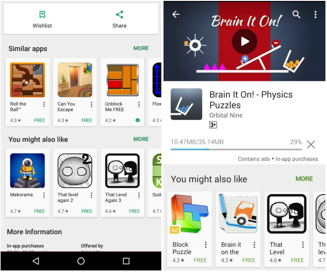
These app topic classifiers enable search and discovery features in the Google Play Apps store. The current system helps provide relevant results to our users, but we are constantly exploring new ways to improve the system, through additional signals, architectural improvements and new algorithms. In Part 2 of this series, we will discuss how to personalize the app discovery experience for users.

Acknowledgments
This work was done within the Google Play team in close collaboration with Liadan O'Callaghan, Yuhua Zhu, Mark Taylor and Michael Watson.