Tag Archives: datasets

The Data Cards Playbook: A Toolkit for Transparency in Dataset Documentation

Posted by Mahima Pushkarna, Senior Interaction Designer, and Andrew Zaldivar, Senior Developer Relations Engineer, Google Research

As machine learning (ML) research moves toward large-scale models capable of numerous downstream tasks, a shared understanding of a dataset’s origin, development, intent, and evolution becomes increasingly important for the responsible and informed development of ML models. However, knowledge about datasets, including use and implementations, is often distributed across teams, individuals, and even time. Earlier this year at the ACM Conference on Fairness, Accountability, and Transparency (ACM FAccT), we published Data Cards, a dataset documentation framework aimed at increasing transparency across dataset lifecycles. Data Cards are transparency artifacts that provide structured summaries of ML datasets with explanations of processes and rationale that shape the data and describe how the data may be used to train or evaluate models. At minimum, Data Cards include the following: (1) upstream sources, (2) data collection and annotation methods, (3) training and evaluation methods, (4) intended use, and (5) decisions affecting model performance.

In practice, two critical factors determine the success of a transparency artifact, the ability to identify the information decision-makers use and the establishment of processes and guidance needed to acquire that information. We started to explore this idea in our paper with three “scaffolding” frameworks designed to adapt Data Cards to a variety of datasets and organizational contexts. These frameworks helped us create boundary infrastructures, which are the processes and engagement models that complement technical and functional infrastructure necessary to communicate information between communities of practice. Boundary infrastructures enable dataset stakeholders to find common ground used to provide diverse input into decisions for the creation, documentation, and use of datasets.

Today, we introduce the Data Cards Playbook, a self-guided toolkit for a variety of teams to navigate transparency challenges with their ML datasets. The Playbook applies a human-centered design approach to documentation — from planning a transparency strategy and defining the audience to writing reader-centric summaries of complex datasets — to ensure that the usability and utility of the documented datasets are well understood. We’ve created participatory activities to navigate typical obstacles in setting up a dataset transparency effort, frameworks that can scale data transparency to new data types, and guidance that researchers, product teams and companies can use to produce Data Cards that reflect their organizational principles.

The Data Cards Playbook incorporates the latest in fairness, accountability, and transparency research.

The Data Cards Playbook

We created the Playbook using a multi-pronged approach that included surveys, artifact analysis, interviews, and workshops. We studied what Googlers wanted to know about datasets and models, and how they used that information in their day-to-day work. Over the past two years, we deployed templates for transparency artifacts used by fifteen teams at Google, and when bottlenecks arose, we partnered with these teams to determine appropriate workarounds. We then created over twenty Data Cards that describe image, language, tabular, video, audio, and relational datasets in production settings, some of which are now available on GitHub. This multi-faceted approach provided insights into the documentation workflows, collaborative information-gathering practices, information requests from downstream stakeholders, and review and assessment practices for each Google team.

Moreover, we spoke with design, policy, and technology experts across the industry and academia to get their unique feedback on the Data Cards we created. We also incorporated our learnings from a series of workshops at ACM FAccT in 2021. Within Google, we evaluated the effectiveness and scalability of our solutions with ML researchers, data scientists, engineers, AI ethics reviewers, product managers, and leadership. In the Data Cards Playbook, we’ve translated successful approaches into repeatable practices that can easily be adapted to unique team needs.

Activities, Foundations, and Transparency Patterns

The Data Cards Playbook is modeled after sprints and co-design practices, so cross-functional teams and their stakeholders can work together to define transparency with an eye for real-world problems they experience when creating dataset documentation and governance solutions. The thirty-three available Activities invite broad, critical perspectives from a wide variety of stakeholders, so Data Cards can be useful for decisions across the dataset lifecycle. We partnered with researchers from the Responsible AI team at Google to create activities that can reflect considerations of fairness and accountability. For example, we've adapted Evaluation Gaps in ML practices into a worksheet for more complete dataset documentation.

Download readily-available activity templates to use the Data Cards Playbook in your organization.

We’ve formed Transparency Patterns with evidence-based guidance to help anticipate challenges faced when producing transparent documentation, offer best practices that improve transparency, and make Data Cards useful for readers from different backgrounds. The challenges and their workarounds are based on data and insights from Googlers, industry experts, and academic research.

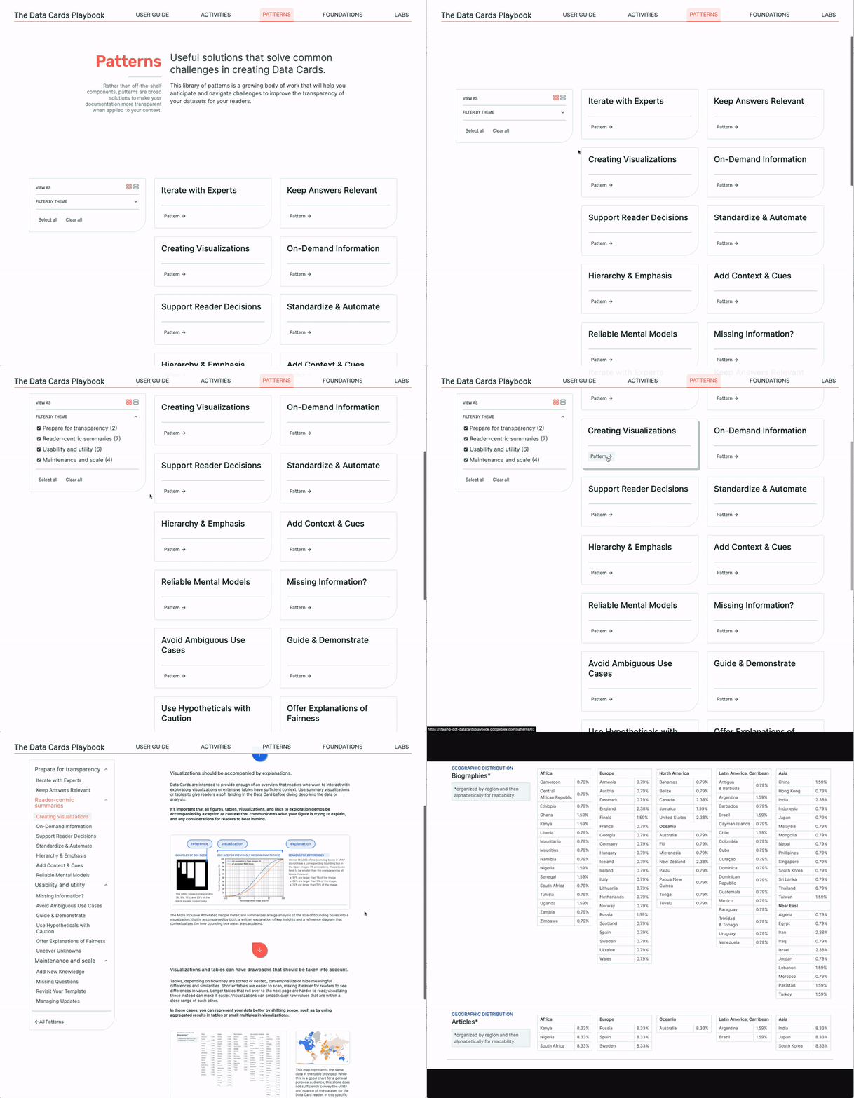
Patterns help unblock teams with recommended practices, caution against common pitfalls, and suggested alternatives to roadblocks.

The Playbook also includes Foundations, which are scalable concepts and frameworks that explore fundamental aspects of transparency as new contexts of data modalities and ML arise. Each Foundation supports different product development stages and includes key takeaways, actions for teams, and handy resources.

Playbook Modules

The Playbook is organized into four modules: (1) Ask, (2) Inspect, (3) Answer, and (3) Audit. Each module contains a growing compendium of materials teams can use within their workflows to tackle transparency challenges that frequently co-occur. Since Data Cards were created with scalability and extensibility in mind, modules leverage divergence-converge thinking that teams may already use, so documentation isn’t an afterthought. The Ask and Inspect modules help create and evaluate Data Card templates for organizational needs and principles. The Answer and Audit modules help data teams complete the templates and evaluate the resulting Data Cards.

In Ask, teams define transparency and optimize their dataset documentation for cross-functional decision-making. Participatory activities create opportunities for Data Card readers to have a say in what constitutes transparency in the dataset’s documentation. These address specific challenges and are rated for different intensities and durations so teams can mix-and-match activities around their needs.

The Inspect module contains activities to identify gaps and opportunities in dataset transparency and processes from user-centric and dataset-centric perspectives. It supports teams in refining, validating, and operationalizing Data Card templates across an organization so readers can arrive at reasonable conclusions about the datasets described.

The Answer module contains transparency patterns and dataset-exploration activities to answer challenging and ambiguous questions. Topics covered include preparing for transparency, writing reader-centric summaries in documentation, unpacking the usability and utility of datasets, and maintaining a Data Card over time.

The Audit module helps data teams and organizations set up processes to evaluate completed Data Cards before they are published. It also contains guidance to measure and track how a transparency effort for multiple datasets scales within organizations.

In Practice

A data operations team at Google used an early version of the Lenses and Scopes Activities from the Ask modules to create a customized Data Card template. Interestingly, we saw them use this template across their workflow till datasets were handed off. They used Data Cards to take dataset requests from research teams, tracked the various processes to create the datasets, collected metadata from vendors responsible for annotations, and managed approvals. Their experiences of iterating with experts and managing updates are reflected in our Transparency Patterns.

Another data governance group used a more advanced version of the activities to interview stakeholders for their ML health-related initiative. Using these descriptions, they identified stakeholders to co-create their Data Card schema. Voting on Lenses was used to rule out typical documentation questions, and identify atypical documentation needs specific to their data type, and important for decisions frequently made by ML leadership and tactical roles within their team. These questions were then used to customize existing metadata schemas in their data repositories.

Conclusion

We present the Data Cards Playbook, a continuous and contextual approach to dataset transparency that deliberately considers all relevant materials and contexts. With this, we hope to establish and promote practice-oriented foundations for transparency to pave the path for researchers to develop ML systems and datasets that are responsible and benefit society.

In addition to the four Playbook modules described, we’re also open-sourcing a card builder, which generates interactive Data Cards from a Markdown file. You can see the builder in action in the GEM Benchmark project’s Data Cards. The Data Cards created were a result of activities from this Playbook, in which the GEM team identified improvements across all dimensions, and created an interactive collection tool designed around scopes.

We acknowledge that this is not a comprehensive solution for fairness, accountability, or transparency in itself. We’ll continue to improve the Playbook using lessons learned. We hope the Data Cards Playbook can become a robust platform for collaboratively advancing transparency research, and invite you to make this your own.

Acknowledgements

This work was done in collaboration with Reena Jana, Vivian Tsai, and Oddur Kjartansson. We want to thank Donald Gonzalez, Dan Nanas, Parker Barnes, Laura Rosenstein, Diana Akrong, Monica Caraway, Ding Wang, Danielle Smalls, Aybuke Turker, Emily Brouillet, Andrew Fuchs, Sebastian Gehrmann, Cassie Kozyrkov, Alex Siegman, and Anthony Keene for their immense contributions; and Meg Mitchell and Timnit Gebru for championing this work.

We also want to thank Adam Boulanger, Lauren Wilcox, Roxanne Pinto, Parker Barnes, and Ayça Çakmakli for their feedback; Tulsee Doshi, Dan Liebling, Meredith Morris, Lucas Dixon, Fernanda Viegas, Jen Gennai, and Marian Croak for their support. This work would not have been possible without our workshop and study participants, and numerous partners, whose insights and experiences have shaped this Playbook.

Source: Google AI Blog

Open Images V7 — Now Featuring Point Labels

Posted by Rodrigo Benenson, Research Scientist, Google Research

Open Images is a computer vision dataset covering ~9 million images with labels spanning thousands of object categories. Researchers around the world use Open Images to train and evaluate computer vision models. Since the initial release of Open Images in 2016, which included image-level labels covering 6k categories, we have provided multiple updates to enrich annotations and expand the potential use cases of the dataset. Through several releases, we have added image-level labels for over 20k categories on all images and bounding box annotations, visual relations, instance segmentations, and localized narratives (synchronized voice, mouse trace, and text caption) on a subset of 1.9M images.

Today, we are happy to announce the release of Open Images V7, which expands the Open Images dataset even further with a new annotation type called point-level labels and includes a new all-in-one visualization tool that allows a better exploration of the rich data available.

Point Labels

The main strategy used to collect the new point-level label annotations leveraged suggestions from a machine learning (ML) model and human verification. First, the ML model selected points of interest and asked a yes or no question, e.g., “is this point on a pumpkin?”. Then, human annotators spent an average of 1.1 seconds answering the yes or no questions. We aggregated the answers from different annotators over the same question and assigned a final “yes”, “no”, or “unsure” label to each annotated point.

Illustration of the annotations interface.
(Image by Lenore Edman, under CC BY 2.0 license)

For each annotated image, we provide a collection of points, each with a “yes” or “no” label for a given class. These points provide sparse information that can be used for the semantic segmentation task. We collected a total of 38.6M new point annotations (12.4M with “yes” labels) that cover 5.8 thousand classes and 1.4M images.

By focusing on point labels, we expanded the number of images annotated and categories covered. We also concentrated the efforts of our annotators on efficiently collecting useful information. Compared to our instance segmentation, the new points include 16x more classes and cover more images. The new points also cover 9x more classes than our box annotations. Compared to existing segmentation datasets, like PASCAL VOC, COCO, Cityscapes, LVIS, or ADE20K, our annotations cover more classes and more images than previous work. The new point label annotations are the first type of annotation in Open Images that provides localization information for both things (countable objects, like cars, cats, and catamarans), and stuff categories (uncountable objects like grass, granite, and gravel). Overall, the newly collected data is roughly equivalent to two years of human annotation effort.

Our initial experiments show that this type of sparse data is suitable for both training and evaluating segmentation models. Training a model directly on sparse data allows us to reach comparable quality to training on dense annotations. Similarly, we show that one can directly compute the traditional semantic segmentation intersection-over-union (IoU) metric over sparse data. The ranking across different methods is preserved, and the sparse IoU values are an accurate estimate of its dense version. See our paper for more details.

Below, we show four example images with their point-level labels, illustrating the rich and diverse information these annotations provide. Circles ⭘ are “yes” labels, and squares ☐ are “no” labels.

Four example images with point-level labels.
Images by Richie Diesterheft, John AM Nueva, Sarah Ackerman, and C Thomas, all under CC BY 2.0 license.

New Visualizers

In addition to the new data release, we also expanded the available visualizations of the Open Images annotations. The Open Images website now includes dedicated visualizers to explore the localized narratives annotations, the new point-level annotations, and a new all-in-one view. This new all-in-one view is available for the subset of 1.9M densely annotated images and allows one to explore the rich annotations that Open Images has accumulated over seven releases. On average these images have annotations for 6.7 image-labels (classes), 8.3 boxes, 1.7 relations, 1.5 masks, 0.4 localized narratives and 34.8 point-labels per image.

Below, we show two example images with various annotations in the all-in-one visualizer. The figures show the image-level labels, bounding boxes, box relations, instance masks, localized narrative mouse trace and caption, and point-level labels. The + classes have positive annotations (of any kind), while – classes have only negative annotations (image-level or point-level).

Two example images with various annotations in the all-in-one visualizer.
Images by Jason Paris, and Rubén Vique, all under CC BY 2.0 license.

Conclusion

We hope that this new data release will enable computer vision research to cover ever more diverse and challenging scenarios. As the quality of automated semantic segmentation models improves over common classes, we want to move towards the long tail of visual concepts, and sparse point annotations are a step in that direction. More and more works are exploring how to use such sparse annotations (e.g., as supervision for instance segmentation or semantic segmentation), and Open Images V7 contributes to this research direction. We are looking forward to seeing what you will build next.

Acknowledgements

Thanks to Vittorio Ferrari, Jordi Pont-Tuset, Alina Kuznetsova, Ashlesha Sadras, and the annotators team for their support creating this new data release.

Source: Google AI Blog

Crossmodal-3600 — Multilingual Reference Captions for Geographically Diverse Images

Posted by Ashish Thapliyal, Software Engineer, and Jordi Pont-Tuset, Research Scientist, Google Research

Image captioning is the machine learning task of automatically generating a fluent natural language description for a given image. This task is important for improving accessibility for visually impaired users and is a core task in multimodal research encompassing both vision and language modeling.

However, datasets for image captioning are primarily available in English. Beyond that, there are only a few datasets covering a limited number of languages that represent just a small fraction of the world’s population. Further, these datasets feature images that severely under-represent the richness and diversity of cultures from across the globe. These aspects have hindered research on image captioning for a wide variety of languages, and directly hamper the deployment of accessibility solutions for a large potential audience around the world.

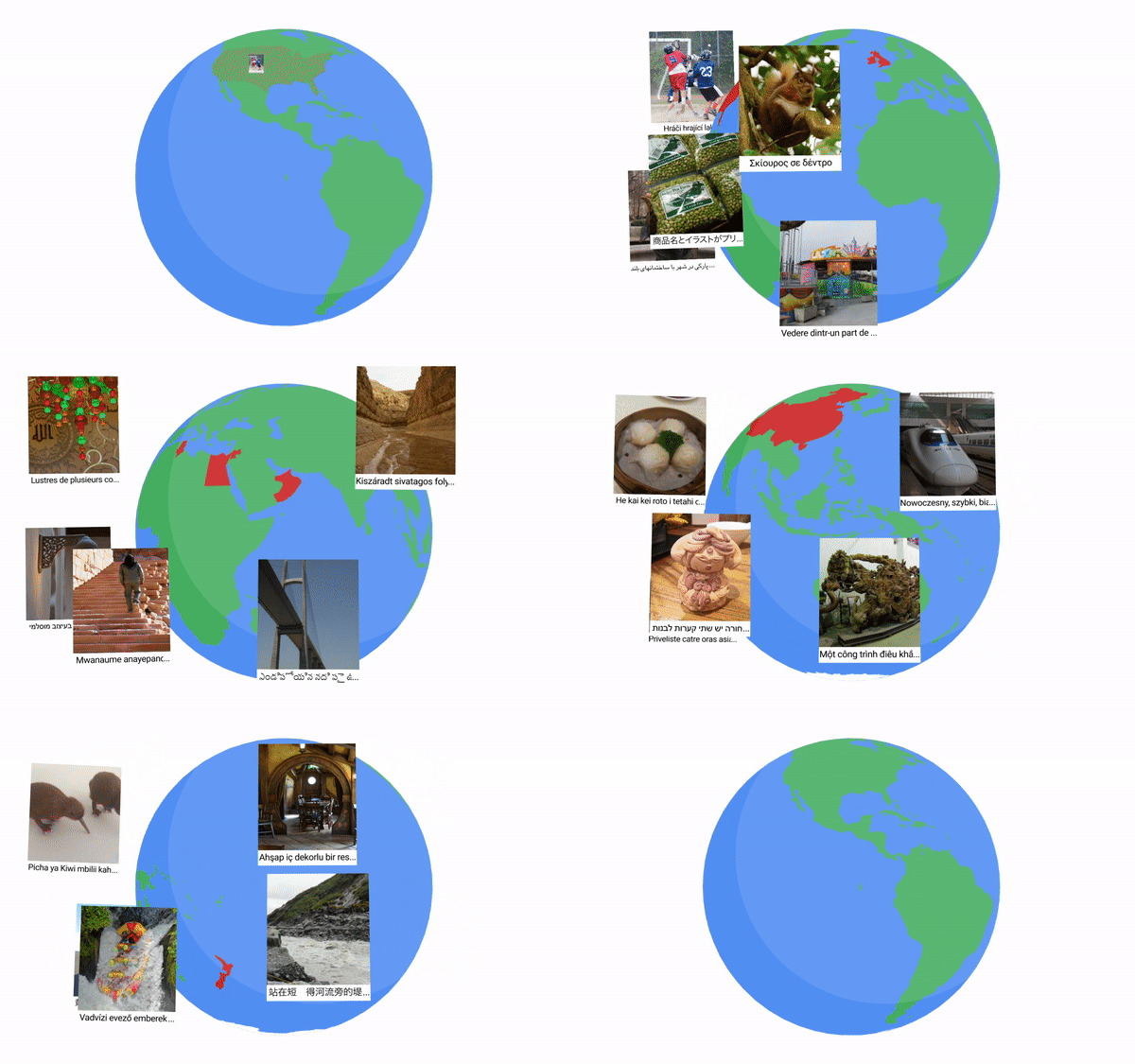
Today we present and make publicly available the Crossmodal 3600 (XM3600) image captioning evaluation dataset as a robust benchmark for multilingual image captioning that enables researchers to reliably compare research contributions in this emerging field. XM3600 provides 261,375 human-generated reference captions in 36 languages for a geographically diverse set of 3600 images. We show that the captions are of high quality and the style is consistent across languages.

The Crossmodal 3600 dataset includes reference captions in 36 languages for each of a geographically diverse set of 3600 images. All images used with permission under the CC-BY 2.0 license.

Overview of the Crossmodal 3600 Dataset
Creating large training and evaluation datasets in multiple languages is a resource-intensive endeavor. Recent work has shown that it is feasible to build multilingual image captioning models trained on machine-translated data with English captions as the starting point. However, some of the most reliable automatic metrics for image captioning are much less effective when applied to evaluation sets with translated image captions, resulting in poorer agreement with human evaluations compared to the English case. As such, trustworthy model evaluation at present can only be based on extensive human evaluation. Unfortunately, such evaluations usually cannot be replicated across different research efforts, and therefore do not offer a fast and reliable mechanism to automatically evaluate multiple model parameters and configurations (e.g., model hill climbing) or to compare multiple lines of research.

XM3600 provides 261,375 human-generated reference captions in 36 languages for a geographically diverse set of 3600 images from the Open Images dataset. We measure the quality of generated captions by comparing them to the manually provided captions using the CIDEr metric, which ranges from 0 (unrelated to the reference captions) to 10 (perfectly matching the reference captions). When comparing pairs of models, we observed strong correlations between the differences in the CIDEr scores of the model outputs, and side-by-side human evaluations comparing the model outputs. , making XM3600 is a reliable tool for high-quality automatic comparisons between image captioning models on a wide variety of languages beyond English.

Language Selection
We chose 30 languages beyond English, roughly based on their percentage of web content. In addition, we chose an additional five languages that include under-resourced languages that have many native speakers or major native languages from continents that would not be covered otherwise. Finally, we also included English as a baseline, thus resulting in a total of 36 languages, as listed in the table below.

Arabic	Bengali*	Chinese	Croatian	Cusco Quechua*	Czech
Danish	Dutch	English	Filipino	Finnish	French
German	Greek	Hebrew	Hindi	Hungarian	Indonesian
Italian	Japanese	Korean	Maori*	Norwegian	Persian
Polish	Portuguese	Romanian	Russian	Spanish	Swahili*
Swedish	Telugu*	Thai	Turkish	Ukrainian	Vietnamese

List of languages used in XM3600. *Low-resource languages with many native speakers, or major native languages from continents that would not be covered otherwise.

Image Selection
The images were selected from among those in the Open Images dataset that have location metadata. Since there are many regions where more than one language is spoken, and some areas are not well covered by these images, we designed an algorithm to maximize the correspondence between selected images and the regions where the targeted languages are spoken. The algorithm starts with the selection of images with geo-data corresponding to the languages for which we have the smallest pool (e.g., Persian) and processes them in increasing order of their candidate image pool size. If there aren't enough images in an area where a language is spoken, then we gradually expand the geographic selection radius to: (i) a country where the language is spoken; (ii) a continent where the language is spoken; and, as last resort, (iii) from anywhere in the world. This strategy succeeded in providing our target number of 100 images from an appropriate region for most of the 36 languages, except for Persian (where 14 continent-level images are used) and Hindi (where all 100 images are at the global level, because the in-region images were assigned to Bengali and Telugu).

English Photo by Chris Sampson	Swahili Photo by Henrik Palm	Telugu Photo by rojypala

Cusco Quechua Photo by McKay Savage	Filipino Photo by Simon Schoeters	Chinese Photo by Stefan Krasowski

Sample images showcasing the geographical diversity of the annotated images. Images used under CC BY 2.0 license.

Caption Generation
In total, all 3600 images (100 images per language) are annotated in all 36 languages, each with an average of two annotations per language, yielding a total of 261,375 captions.

Annotators work in batches of 15 images. The first screen shows all 15 images with their captions in English as generated by a captioning model trained to output a consistent style of the form "<main salient objects> doing <activities> in the <environment>", often with object attributes, such as a "smiling" person, "red" car, etc. The annotators are asked to rate the caption quality given guidelines for a 4-point scale from "excellent" to "bad", plus an option for "not_enough_information". This step forces the annotators to carefully assess caption quality and it primes them to internalize the style of the captions. The following screens show the images again but individually and without the English captions, and the annotators are asked to produce descriptive captions in the target language for each image.

The image batch size of 15 was chosen so that the annotators would internalize the style without remembering the exact captions. Thus, we expect the raters to generate captions based on the image content only and lacking translation artifacts. For example in the example shown below, the Spanish caption mentions “number 42” and the Thai caption mentions “convertibles”, none of which are mentioned in the English captions. The annotators were also provided with a protocol to use when creating the captions, thus achieving style consistency across languages.

Photo by Brian Solis	English	• A vintage sports car in a showroom with many other vintage sports cars
		• The branded classic cars in a row at display

	Spanish	• Automóvil clásico deportivo en exhibición de automóviles de galería — (Classic sports car in gallery car show)
		• Coche pequeño de carreras color plateado con el número 42 en una exhibición de coches — (Small silver racing car with the number 42 at a car show)

	Thai	• รถเปิดประทุนหลายสีจอดเรียงกันในที่จัดแสดง — (Multicolored convertibles line up in the exhibit)
		• รถแข่งวินเทจจอดเรียงกันหลายคันในงานจัดแสดง — (Several vintage racing cars line up at the show.)

Sample captions in three different languages (out of 36 — see full list of captions in Appendix A of the Crossmodal-3600 paper), showcasing the creation of annotations that are consistent in style across languages, while being free of direct-translation artifacts (e.g., the Spanish “number 42” or the Thai “convertibles” would not be possible when directly translating from the English versions). Image used under CC BY 2.0 license.

Caption Quality and Statistics
We ran two to five pilot studies per language to troubleshoot the caption generation process and to ensure high quality captions. We then manually evaluated a random subset of captions. First we randomly selected a sample of 600 images. Then, to measure the quality of captions in a particular language, for each image, we selected for evaluation one of the manually generated captions. We found that:

For 25 out of 36 languages, the percentage of captions rated as “Good” or “Excellent” is above 90%, and the rest are all above 70%.
For 26 out of 36 languages, the percentage of captions rated as “Bad” is below 2%, and the rest are all below 5%.

For languages that use spaces to separate words, the number of words per caption can be as low as 5 or 6 for some agglutinative languages like Cusco Quechua and Czech, and as high as 18 for an analytic language like Vietnamese. The number of characters per caption also varies drastically — from mid-20s for Korean to mid-90s for Indonesian — depending on the alphabet and the script of the language.

Empirical Evaluation and Results
We empirically measured the ability of the XM3600 annotations to rank image captioning model variations by training four variations of a multilingual image captioning model and comparing the CIDEr differences of the models’ outputs over the XM3600 dataset for 30+ languages, to side-by-side human evaluations. We observed strong correlations between the CIDEr differences and the human evaluations. These results support the use of the XM3600 references as a means to achieve high-quality automatic comparisons between image captioning models on a wide variety of languages beyond English.

Recent Uses
Recently PaLI used XM3600 to evaluate model performance beyond English for image captioning, image-to-text retrieval and text-to-image retrieval. The key takeaways they found when evaluating on XM3600 were that multilingual captioning greatly benefits from scaling the PaLI models, especially for low-resource languages.

Acknowledgements
We would like to acknowledge the coauthors of this work: Xi Chen and Radu Soricut.

Source: Google AI Blog

TensorStore for High-Performance, Scalable Array Storage

Posted by Jeremy Maitin-Shepard and Laramie Leavitt, Software Engineers, Connectomics at Google

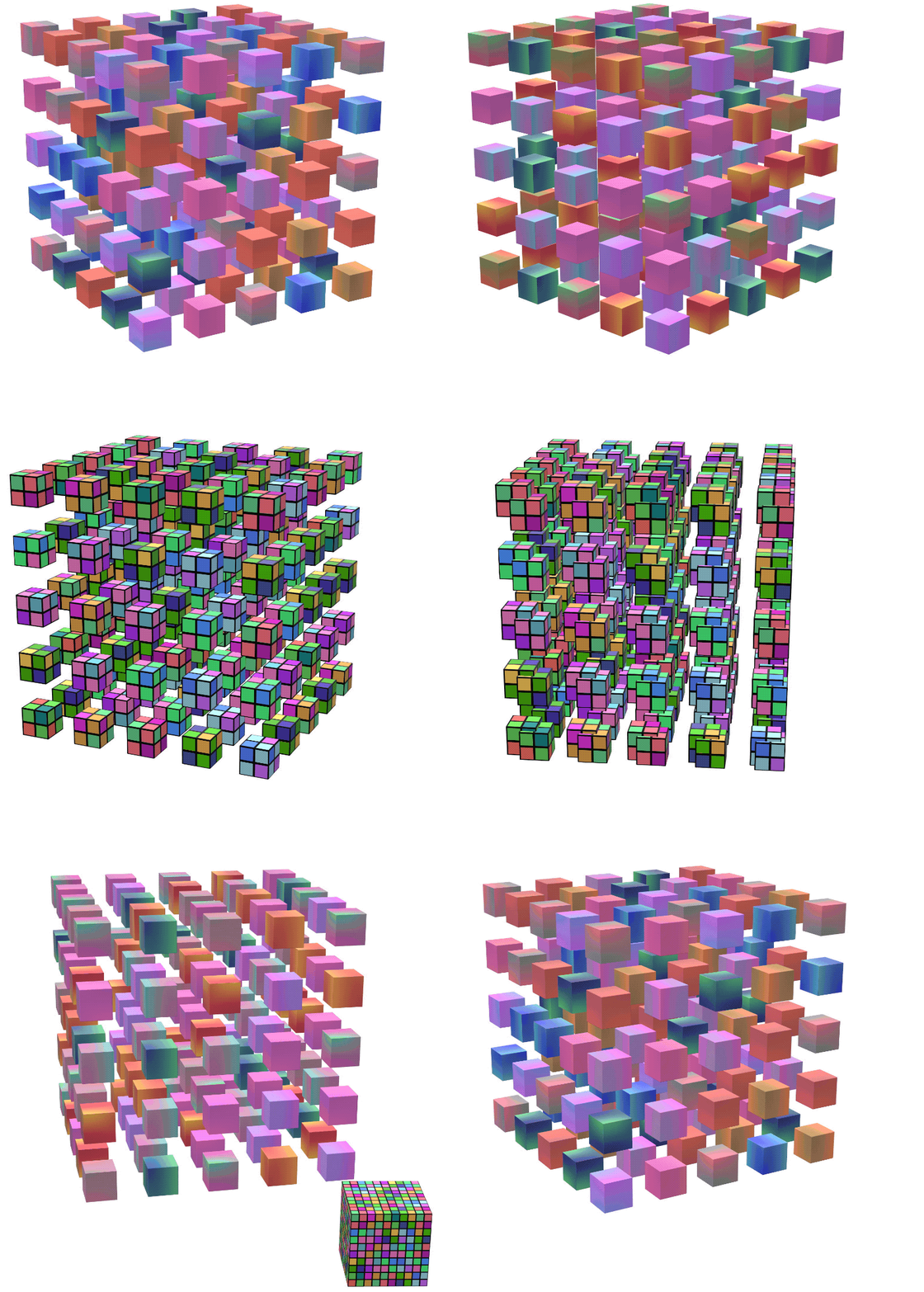
Many exciting contemporary applications of computer science and machine learning (ML) manipulate multidimensional datasets that span a single large coordinate system, for example, weather modeling from atmospheric measurements over a spatial grid or medical imaging predictions from multi-channel image intensity values in a 2d or 3d scan. In these settings, even a single dataset may require terabytes or petabytes of data storage. Such datasets are also challenging to work with as users may read and write data at irregular intervals and varying scales, and are often interested in performing analyses using numerous machines working in parallel.

Today we are introducing TensorStore, an open-source C++ and Python software library designed for storage and manipulation of n-dimensional data that:

Provides a uniform API for reading and writing multiple array formats, including zarr and N5.
Natively supports multiple storage systems, including Google Cloud Storage, local and network filesystems, HTTP servers, and in-memory storage.
Supports read/writeback caching and transactions, with strong atomicity, isolation, consistency, and durability (ACID) guarantees.
Supports safe, efficient access from multiple processes and machines via optimistic concurrency.
Offers an asynchronous API to enable high-throughput access even to high-latency remote storage.
Provides advanced, fully composable indexing operations and virtual views.

TensorStore has already been used to solve key engineering challenges in scientific computing (e.g., management and processing of large datasets in neuroscience, such as peta-scale 3d electron microscopy data and “4d” videos of neuronal activity). TensorStore has also been used in the creation of large-scale machine learning models such as PaLM by addressing the problem of managing model parameters (checkpoints) during distributed training.

Familiar API for Data Access and Manipulation
TensorStore provides a simple Python API for loading and manipulating large array data. In the following example, we create a TensorStore object that represents a 56 trillion voxel 3d image of a fly brain and access a small 100x100 patch of the data as a NumPy array:

>>> import tensorstore as ts
>>> import numpy as np

# Create a TensorStore object to work with fly brain data.
>>> dataset = ts.open({
...     'driver':
...         'neuroglancer_precomputed',
...     'kvstore':
...         'gs://neuroglancer-janelia-flyem-hemibrain/v1.1/segmentation/',
... }).result()

# Create a 3-d view (remove singleton 'channel' dimension):
>>> dataset_3d = dataset[ts.d['channel'][0]]
>>> dataset_3d.domain
{ "x": [0, 34432), "y": [0, 39552), "z": [0, 41408) }

# Convert a 100x100x1 slice of the data to a numpy ndarray
>>> slice = np.array(dataset_3d[15000:15100, 15000:15100, 20000])

Crucially, no actual data is accessed or stored in memory until the specific 100x100 slice is requested; hence arbitrarily large underlying datasets can be loaded and manipulated without having to store the entire dataset in memory, using indexing and manipulation syntax largely identical to standard NumPy operations. TensorStore also provides extensive support for advanced indexing features, including transforms, alignment, broadcasting, and virtual views (data type conversion, downsampling, lazily on-the-fly generated arrays).

The following example demonstrates how TensorStore can be used to create a zarr array, and how its asynchronous API enables higher throughput:

>>> import tensorstore as ts
>>> import numpy as np

>>> # Create a zarr array on the local filesystem
>>> dataset = ts.open({
...     'driver': 'zarr',
...     'kvstore': 'file:///tmp/my_dataset/',
... },
... dtype=ts.uint32,
... chunk_layout=ts.ChunkLayout(chunk_shape=[256, 256, 1]),
... create=True,
... shape=[5000, 6000, 7000]).result()

>>> # Create two numpy arrays with example data to write.
>>> a = np.arange(100*200*300, dtype=np.uint32).reshape((100, 200, 300))
>>> b = np.arange(200*300*400, dtype=np.uint32).reshape((200, 300, 400))

>>> # Initiate two asynchronous writes, to be performed concurrently.
>>> future_a = dataset[1000:1100, 2000:2200, 3000:3300].write(a)
>>> future_b = dataset[3000:3200, 4000:4300, 5000:5400].write(b)

>>> # Wait for the asynchronous writes to complete
>>> future_a.result()
>>> future_b.result()

Safe and Performant Scaling
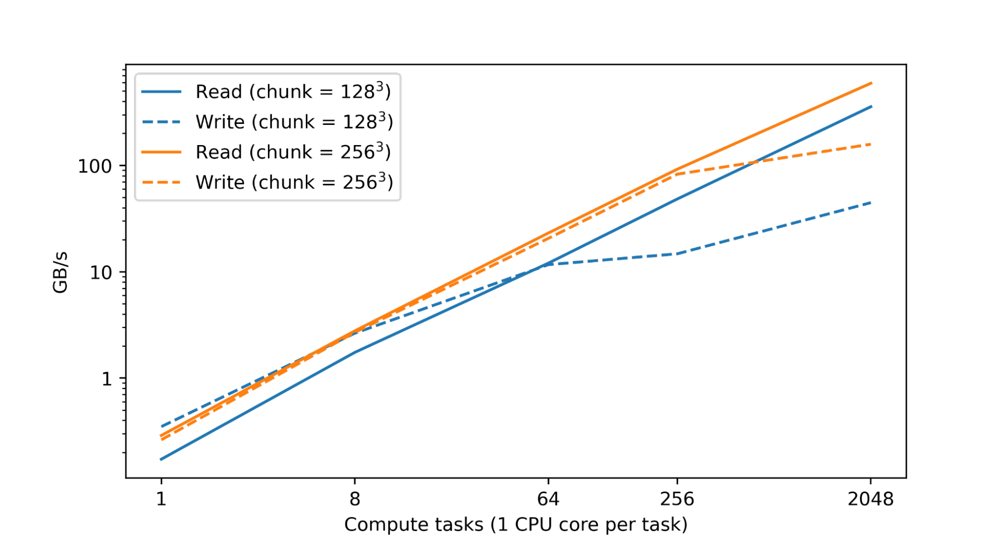
Processing and analyzing large numerical datasets requires significant computational resources. This is typically achieved through parallelization across numerous CPU or accelerator cores spread across many machines. Therefore a fundamental goal of TensorStore has been to enable parallel processing of individual datasets that is both safe (i.e., avoids corruption or inconsistencies arising from parallel access patterns) and high performance (i.e., reading and writing to TensorStore is not a bottleneck during computation). In fact, in a test within Google’s datacenters, we found nearly linear scaling of read and write performance as the number of CPUs was increased:

Read and write performance for a TensorStore dataset in zarr format residing on Google Cloud Storage (GCS) accessed concurrently using a variable number of single-core compute tasks in Google data centers. Both read and write performance scales nearly linearly with the number of compute tasks.

Performance is achieved by implementing core operations in C++, extensive use of multithreading for operations such as encoding/decoding and network I/O, and partitioning large datasets into much smaller units through chunking to enable efficiently reading and writing subsets of the entire dataset. TensorStore also provides configurable in-memory caching (which reduces slower storage system interactions for frequently accessed data) and an asynchronous API that enables a read or write operation to continue in the background while a program completes other work.

Safety of parallel operations when many machines are accessing the same dataset is achieved through the use of optimistic concurrency, which maintains compatibility with diverse underlying storage layers (including Cloud storage platforms, such as GCS, as well as local filesystems) without significantly impacting performance. TensorStore also provides strong ACID guarantees for all individual operations executing within a single runtime.

To make distributed computing with TensorStore compatible with many existing data processing workflows, we have also integrated TensorStore with parallel computing libraries such as Apache Beam (example code) and Dask (example code).

Use Case: Language Models
An exciting recent development in ML is the emergence of more advanced language models such as PaLM. These neural networks contain hundreds of billions of parameters and exhibit some surprising capabilities in natural language understanding and generation. These models also push the limits of computational infrastructure; in particular, training a language model such as PaLM requires thousands of TPUs working in parallel.

One challenge that arises during this training process is efficiently reading and writing the model parameters. Training is distributed across many separate machines, but parameters must be regularly saved to a single object (“checkpoint”) on a permanent storage system without slowing down the overall training process. Individual training jobs must also be able to read just the specific set of parameters they are concerned with in order to avoid the overhead that would be required to load the entire set of model parameters (which could be hundreds of gigabytes).

TensorStore has already been used to address these challenges. It has been applied to manage checkpoints associated with large-scale (“multipod”) models trained with JAX (code example) and has been integrated with frameworks such as T5X (code example) and Pathways. Model parallelism is used to partition the full set of parameters, which can occupy more than a terabyte of memory, over hundreds of TPUs. Checkpoints are stored in zarr format using TensorStore, with a chunk structure chosen to allow the partition for each TPU to be read and written independently in parallel.

When saving a checkpoint, each model parameter is written using TensorStore in zarr format using a chunk grid that further subdivides the grid used to partition the parameter over TPUs. The host machines write in parallel the zarr chunks for each of the partitions assigned to TPUs attached to that host. Using TensorStore's asynchronous API, training proceeds even while the data is still being written to persistent storage. When resuming from a checkpoint, each host reads only the chunks that make up the partitions assigned to that host.

Use Case: 3D Brain Mapping
The field of synapse-resolution connectomics aims to map the wiring of animal and human brains at the detailed level of individual synaptic connections. This requires imaging the brain at extremely high resolution (nanometers) over fields of view of up to millimeters or more, which yields datasets that can span petabytes in size. In the future these datasets may extend to exabytes as scientists contemplate mapping entire mouse or primate brains. However, even current datasets pose significant challenges related to storage, manipulation, and processing; in particular, even a single brain sample may require millions of gigabytes with a coordinate system (pixel space) of hundreds of thousands pixels in each dimension.

We have used TensorStore to solve computational challenges associated with large-scale connectomic datasets. Specifically, TensorStore has managed some of the largest and most widely accessed connectomic datasets, with Google Cloud Storage as the underlying object storage system. For example, it has been applied to the human cortex “h01” dataset, which is a 3d nanometer-resolution image of human brain tissue. The raw imaging data is 1.4 petabytes (roughly 500,000 * 350,000 * 5,000 pixels large, and is further associated with additional content such as 3d segmentations and annotations that reside in the same coordinate system. The raw data is subdivided into individual chunks 128x128x16 pixels large and stored in the “Neuroglancer precomputed” format, which is optimized for web-based interactive viewing and can be easily manipulated from TensorStore.

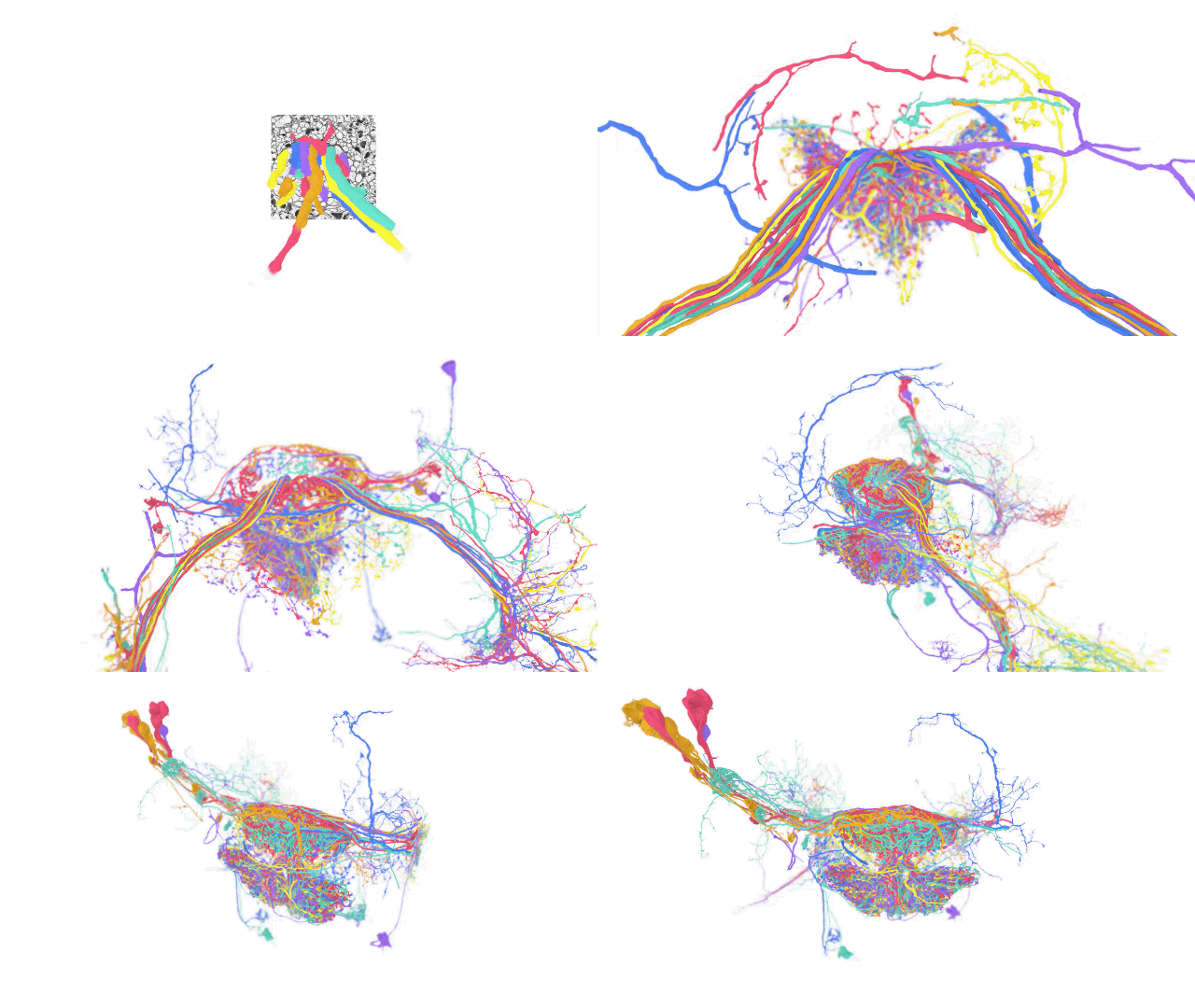
A fly brain reconstruction for which the underlying data can be easily accessed and manipulated using TensorStore.

Getting Started
To get started using the TensorStore Python API, you can install the tensorstore PyPI package using:

pip install tensorstore

Refer to the tutorials and API documentation for usage details. For other installation options and for using the C++ API, refer to installation instructions.

Acknowledgements
Thanks to Tim Blakely, Viren Jain, Yash Katariya, Jan-Matthis Luckmann, Michał Januszewski, Peter Li, Adam Roberts, Brain Williams, and Hector Yee from Google Research, and Davis Bennet, Stuart Berg, Eric Perlman, Stephen Plaza, and Juan Nunez-Iglesias from the broader scientific community for valuable feedback on the design, early testing and debugging.

Source: Google AI Blog

Announcing the Patent Phrase Similarity Dataset

Posted Grigor Aslanyan, Software Engineer, Google

Patent documents typically use legal and highly technical language, with context-dependent terms that may have meanings quite different from colloquial usage and even between different documents. The process of using traditional patent search methods (e.g., keyword searching) to search through the corpus of over one hundred million patent documents can be tedious and result in many missed results due to the broad and non-standard language used. For example, a "soccer ball" may be described as a "spherical recreation device", "inflatable sportsball" or "ball for ball game". Additionally, the language used in some patent documents may obfuscate terms to their advantage, so more powerful natural language processing (NLP) and semantic similarity understanding can give everyone access to do a thorough search.

The patent domain (and more general technical literature like scientific publications) poses unique challenges for NLP modeling due to its use of legal and technical terms. While there are multiple commonly used general-purpose semantic textual similarity (STS) benchmark datasets (e.g., STS-B, SICK, MRPC, PIT), to the best of our knowledge, there are currently no datasets focused on technical concepts found in patents and scientific publications (the somewhat related BioASQ challenge contains a biomedical question answering task). Moreover, with the continuing growth in size of the patent corpus (millions of new patents are issued worldwide every year), there is a need to develop more useful NLP models for this domain.

Today, we announce the release of the Patent Phrase Similarity dataset, a new human-rated contextual phrase-to-phrase semantic matching dataset, and the accompanying paper, presented at the SIGIR PatentSemTech Workshop, which focuses on technical terms from patents. The Patent Phrase Similarity dataset contains ~50,000 rated phrase pairs, each with a Cooperative Patent Classification (CPC) class as context. In addition to similarity scores that are typically included in other benchmark datasets, we include granular rating classes similar to WordNet, such as synonym, antonym, hypernym, hyponym, holonym, meronym, and domain related. This dataset (distributed under the Creative Commons Attribution 4.0 International license) was used by Kaggle and USPTO as the benchmark dataset in the U.S. Patent Phrase to Phrase Matching competition to draw more attention to the performance of machine learning models on technical text. Initial results show that models fine-tuned on this new dataset perform substantially better than general pre-trained models without fine-tuning.

The Patent Phrase Similarity Dataset
To better train the next generation of state-of-the-art models, we created the Patent Phrase Similarity dataset, which includes many examples to address the following problems: (1) phrase disambiguation, (2) adversarial keyword matching, and (3) hard negative keywords (i.e., keywords that are unrelated but received a high score for similarity from other models ). Some keywords and phrases can have multiple meanings (e.g., the phrase "mouse" may refer to an animal or a computer input device), so we disambiguate the phrases by including CPC classes with each pair of phrases. Also, many NLP models (e.g., bag of words models) will not do well on data with phrases that have matching keywords but are otherwise unrelated (adversarial keywords, e.g., “container section” → “kitchen container”, “offset table” → “table fan”). The Patent Phrase Similarity dataset is designed to include many examples of matching keywords that are unrelated through adversarial keyword match, enabling NLP models to improve their performance.

Each entry in the Patent Phrase Similarity dataset contains two phrases, an anchor and target, a context CPC class, a rating class, and a similarity score. The dataset contains 48,548 entries with 973 unique anchors, split into training (75%), validation (5%), and test (20%) sets. When splitting the data, all of the entries with the same anchor are kept together in the same set. There are 106 different context CPC classes and all of them are represented in the training set.

Anchor	Target	Context	Rating	Score
acid absorption	absorption of acid	B08	exact	1.0
acid absorption	acid immersion	B08	synonym	0.75
acid absorption	chemically soaked	B08	domain related	0.25
acid absorption	acid reflux	B08	not related	0.0
gasoline blend	petrol blend	C10	synonym	0.75
gasoline blend	fuel blend	C10	hypernym	0.5
gasoline blend	fruit blend	C10	not related	0.0
faucet assembly	water tap	A22	hyponym	0.5
faucet assembly	water supply	A22	holonym	0.25
faucet assembly	school assembly	A22	not related	0.0

A small sample of the dataset with anchor and target phrases, context CPC class (B08: Cleaning, C10: Petroleum, gas, fuel, lubricants, A22: Butchering, processing meat/poultry/fish), a rating class, and a similarity score.

Generating the Dataset
To generate the Patent Phrase Similarity data, we first process the ~140 million patent documents in the Google Patent's corpus and automatically extract important English phrases, which are typically noun phrases (e.g., “fastener”, “lifting assembly”) and functional phrases (e.g., “food processing”, “ink printing”). Next, we filter and keep phrases that appear in at least 100 patents and randomly sample around 1,000 of these filtered phrases, which we call anchor phrases. For each anchor phrase, we find all of the matching patents and all of the CPC classes for those patents. We then randomly sample up to four matching CPC classes, which become the context CPC classes for the specific anchor phrase.

We use two different methods for pre-generating target phrases: (1) partial matching and (2) a masked language model (MLM). For partial matching, we randomly select phrases from the entire corpus that partially match with the anchor phrase (e.g., “abatement” → “noise abatement”, “material formation” → “formation material”). For MLM, we select sentences from the patents that contain a given anchor phrase, mask them out, and use the Patent-BERT model to predict candidates for the masked portion of the text. Then, all of the phrases are cleaned up, which includes lowercasing and the removal of punctuation and certain stopwords (e.g., "and", "or", "said"), and sent to expert raters for review. Each phrase pair is rated independently by two raters skilled in the technology area. Each rater also generates new target phrases with different ratings. Specifically, they are asked to generate some low-similarity and unrelated targets that partially match with the original anchor and/or some high-similarity targets. Finally, the raters meet to discuss their ratings and come up with final ratings.

Dataset Evaluation
To evaluate its performance, the Patent Phrase Similarity dataset was used in the U.S. Patent Phrase to Phrase Matching Kaggle competition. The competition was very popular, drawing about 2,000 competitors from around the world. A variety of approaches were successfully used by the top scoring teams, including ensemble models of BERT variants and prompting (see the full discussion for more details). The table below shows the best results from the competition, as well as several off-the-shelf baselines from our paper. The Pearson correlation metric was used to measure the linear correlation between the predicted and true scores, which is a helpful metric to target for downstream models so they can distinguish between different similarity ratings.

The baselines in the paper can be considered zero-shot in the sense that they use off-the-shelf models without any further fine-tuning on the new dataset (we use these models to embed the anchor and target phrases separately and compute the cosine similarity between them). The Kaggle competition results demonstrate that by using our training data, one can achieve significant improvements compared with existing NLP models. We have also estimated human performance on this task by comparing a single rater’s scores to the combined score of both raters. The results indicate that this is not a particularly easy task, even for human experts.

Model	Training	Pearson correlation
word2vec	Zero-shot	0.44
Patent-BERT	Zero-shot	0.53
Sentence-BERT	Zero-shot	0.60
Kaggle 1st place single	Fine-tuned	0.87
Kaggle 1st place ensemble	Fine-tuned	0.88
Human		0.93

Performance of popular models with no fine-tuning (zero-shot), models fine-tuned on the Patent Phrase Similarity dataset as part of the Kaggle competition, and single human performance.

Conclusion and Future Work
We present the Patent Phrase Similarity dataset, which was used as the benchmark dataset in the U.S. Patent Phrase to Phrase Matching competition, and demonstrate that by using our training data, one can achieve significant improvements compared with existing NLP models.

Additional challenging machine learning benchmarks can be generated from the patent corpus, and patent data has made its way into many of today's most-studied models. For example, the C4 text dataset used to train T5 contains many patent documents. The BigBird and LongT5 models also use patents via the BIGPATENT dataset. The availability, breadth and open usage terms of full text data (see Google Patents Public Datasets) makes patents a unique resource for the research community. Possibilities for future tasks include massively multi-label classification, summarization, information retrieval, image-text similarity, citation graph prediction, and translation. See the paper for more details.

Acknowledgements
This work was possible through a collaboration with Kaggle, Satsyil Corp., USPTO, and MaxVal. Thanks to contributors Ian Wetherbee from Google, Will Cukierski and Maggie Demkin from Kaggle. Thanks to Jerry Ma, Scott Beliveau, and Jamie Holcombe from USPTO and Suja Chittamahalingam from MaxVal for their contributions.

Source: Google AI Blog

UVQ: Measuring YouTube’s Perceptual Video Quality

Posted by Yilin Wang, Staff Software Engineer, YouTube and Feng Yang, Senior Staff Software Engineer, Google Research

Online video sharing platforms, like YouTube, need to understand perceptual video quality (i.e., a user's subjective perception of video quality) in order to better optimize and improve user experience. Video quality assessment (VQA) attempts to build a bridge between video signals and perceptual quality by using objective mathematical models to approximate the subjective opinions of users. Traditional video quality metrics, like peak signal-to-noise ratio (PSNR) and Video Multi-Method Assessment Fusion (VMAF), are reference-based and focus on the relative difference between the target and reference videos. Such metrics, which work best on professionally generated content (e.g., movies), assume the reference video is of pristine quality and that one can induce the target video's absolute quality from the relative difference.

However, the majority of the videos that are uploaded on YouTube are user-generated content (UGC), which bring new challenges due to their remarkably high variability in video content and original quality. Most UGC uploads are non-pristine and the same amount of relative difference could imply very different perceptual quality impacts. For example, people tend to be less sensitive to the distortions of poor quality uploads than of high quality uploads. Thus, reference-based quality scores become inaccurate and inconsistent when used for UGC cases. Additionally, despite the high volume of UGC, there are currently limited UGC video quality assessment (UGC-VQA) datasets with quality labels. Existing UGC-VQA datasets are either small in size (e.g., LIVE-Qualcomm has 208 samples captured from 54 unique scenes), compared with datasets with millions of samples for classification and recognition (e.g., ImageNet and YouTube-8M), or don’t have enough content variability (sampling without considering content information, like LIVE-VQC and KoNViD-1k).

In "Rich Features for Perceptual Quality Assessment of UGC Videos", published at CVPR 2021, we describe how we attempt to solve the UGC quality assessment problem by building a Universal Video Quality (UVQ) model that resembles a subjective quality assessment. The UVQ model uses subnetworks to analyze UGC quality from high-level semantic information to low-level pixel distortions, and provides a reliable quality score with rationale (leveraging comprehensive and interpretable quality labels). Moreover, to advance UGC-VQA and compression research, we enhance the open-sourced YouTube-UGC dataset, which contains 1.5K representative UGC samples from millions of UGC videos (distributed under the Creative Commons license) on YouTube. The updated dataset contains ground-truth labels for both original videos and corresponding transcoded versions, enabling us to better understand the relationship between video content and its perceptual quality.

Subjective Video Quality Assessment
To understand perceptual video quality, we leverage an internal crowd-sourcing platform to collect mean opinion scores (MOS) with a scale of 1–5, where 1 is the lowest quality and 5 is the highest quality, for no-reference use cases. We collect ground-truth labels from the YouTube-UGC dataset and categorize UGC factors that affect quality perception into three high-level categories: (1) content, (2) distortions, and (3) compression. For example, a video with no meaningful content won't receive a high quality MOS. Also, distortions introduced during the video production phase and video compression artifacts introduced by third-party platforms, e.g., transcoding or transmission, will degrade the overall quality.


MOS= 2.052	MOS= 4.457

Left: A video with no meaningful content won't receive a high quality MOS. Right: A video displaying intense sports shows a higher MOS.


MOS= 1.242	MOS= 4.522

Left: A blurry gaming video gets a very low quality MOS. Right: A video with professional rendering (high contrast and sharp edges, usually introduced in the video production phase) shows a high quality MOS.


MOS= 2.372	MOS= 4.646

Left: A heavily compressed video receives a low quality MOS. Right: a video without compression artifacts shows a high quality MOS.

We demonstrate that the left gaming video in the second row of the figure above has the lowest MOS (1.2), even lower than the video with no meaningful content. A possible explanation is that viewers may have higher video quality expectations for videos that have a clear narrative structure, like gaming videos, and the blur artifacts significantly reduce the perceptual quality of the video.

UVQ Model Framework
A common method for evaluating video quality is to design sophisticated features, and then map these features to a MOS. However, designing useful handcrafted features is difficult and time-consuming, even for domain experts. Also, the most useful existing handcrafted features were summarized from limited samples, which may not perform well on broader UGC cases. In contrast, machine learning is becoming more prominent in UGC-VQA because it can automatically learn features from large-scale samples.

A straightforward approach is to train a model from scratch on existing UGC quality datasets. However, this may not be feasible as there are limited quality UGC datasets. To overcome this limitation, we apply a self-supervised learning step to the UVQ model during training. This self-supervised step enables us to learn comprehensive quality-related features, without ground-truth MOS, from millions of raw videos.

Following the quality-related categories summarized from the subjective VQA, we develop the UVQ model with four novel subnetworks. The first three subnetworks, which we call ContentNet, DistortionNet and CompressionNet, are used to extract quality features (i.e., content, distortion and compression), and the fourth subnetwork, called AggregationNet, maps the extracted features to generate a single quality score. ContentNet is trained in a supervised learning fashion with UGC-specific content labels that are generated by the YouTube-8M model. DistortionNet is trained to detect common distortions, e.g., Gaussian blur and white noise of the original frame. CompressionNet focuses on video compression artifacts, whose training data are videos compressed with different bitrates. CompressionNet is trained using two compressed variants of the same content that are fed into the model to predict corresponding compression levels (with a higher score for more noticeable compression artifacts), with the implicit assumption that the higher bitrate version has a lower compression level.

The ContentNet, DistortionNet and CompressionNet subnetworks are trained on large-scale samples without ground-truth quality scores. Since video resolution is also an important quality factor, the resolution-sensitive subnetworks (CompressionNet and DistortionNet) are patch-based (i.e., each input frame is divided into multiple disjointed patches that are processed separately), which makes it possible to capture all detail on native resolution without downscaling. The three subnetworks extract quality features that are then concatenated by the fourth subnetwork, AggregationNet, to predict quality scores with domain ground-truth MOS from YouTube-UGC.

The UVQ training framework.

Analyzing Video Quality with UVQ
After building the UVQ model, we use it to analyze the video quality of samples pulled from YouTube-UGC and demonstrate that its subnetworks can provide a single quality score along with high-level quality indicators that can help us understand quality issues. For example, DistortionNet detects multiple visual artifacts, e.g., jitter and lens blur, for the middle video below, and CompressionNet detects that the bottom video has been heavily compressed.

ContentNet assigns content labels with corresponding probabilities in parentheses, i.e., car (0.58), vehicle (0.42), sports car (0.32), motorsports (0.18), racing (0.11).

DistortionNet detects and categorizes multiple visual distortions with corresponding probabilities in parentheses, i.e., jitter (0.112), color quantization (0.111), lens blur (0.108), denoise (0.107).

CompressionNet detects a high compression level of 0.892 for the video above.

Additionally, UVQ can provide patch-based feedback to locate quality issues. Below, UVQ reports that the quality of the first patch (patch at time t = 1) is good with a low compression level. However, the model identifies heavy compression artifacts in the next patch (patch at time t = 2).


Patch at time t = 1	Patch at time t = 2
Compression level = 0.000	Compression level = 0.904

UVQ detects a sudden quality degradation (high compression level) for a local patch.

In practice, UVQ can generate a video diagnostic report that includes a content description (e.g., strategy video game), distortion analysis (e.g., the video is blurry or pixelated) and compression level (e.g., low or high compression). Below, UVQ reports that the content quality, looking at individual features, is good, but the compression and distortion quality is low. When combining all three features, the overall quality is medium-low. We see that these findings are close to the rationale summarized by internal user experts, demonstrating that UVQ can reason through quality assessments, while providing a single quality score.

UVQ diagnostic report. ContentNet (CT): Video game, strategy video game, World of Warcraft, etc. DistortionNet (DT): multiplicative noise, Gaussian blur, color saturation, pixelate, etc. CompressionNet (CP): 0.559 (medium-high compression). Predicted quality score in [1, 5]: (CT, DT, CP) = (3.901, 3.216, 3.151), (CT+DT+CP) = 3.149 (medium-low quality).

Conclusion
We present the UVQ model, which generates a report with quality scores and insights that can be used to interpret UGC video perceptual quality. UVQ learns comprehensive quality related features from millions of UGC videos and provides a consistent view of quality interpretation for both no-reference and reference cases. To learn more, read our paper or visit our website to see YT-UGC videos and their subjective quality data. We also hope that the enhanced YouTube-UGC dataset enables more research in this space.

Acknowledgements
This work was possible through a collaboration spanning several Google teams. Key contributors include: Balu Adsumilli, Neil Birkbeck, Joong Gon Yim from YouTube and Junjie Ke, Hossein Talebi, Peyman Milanfar from Google Research. Thanks to Ross Wolf, Jayaprasanna Jayaraman, Carena Church, and Jessie Lin for their contributions.

Source: Google AI Blog

UVQ: Measuring YouTube’s Perceptual Video Quality

Posted by Yilin Wang, Staff Software Engineer, YouTube and Feng Yang, Senior Staff Software Engineer, Google Research


MOS= 2.052	MOS= 4.457

Left: A video with no meaningful content won't receive a high quality MOS. Right: A video displaying intense sports shows a higher MOS.


MOS= 1.242	MOS= 4.522


MOS= 2.372	MOS= 4.646

Left: A heavily compressed video receives a low quality MOS. Right: a video without compression artifacts shows a high quality MOS.

The UVQ training framework.

ContentNet assigns content labels with corresponding probabilities in parentheses, i.e., car (0.58), vehicle (0.42), sports car (0.32), motorsports (0.18), racing (0.11).

CompressionNet detects a high compression level of 0.892 for the video above.


Patch at time t = 1	Patch at time t = 2
Compression level = 0.000	Compression level = 0.904

UVQ detects a sudden quality degradation (high compression level) for a local patch.

Source: Google AI Blog

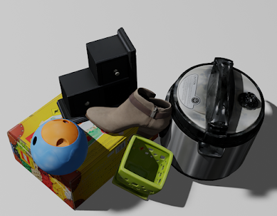
Scanned Objects by Google Research: A Dataset of 3D-Scanned Common Household Items

Posted by Laura Downs and Anthony Francis, Software Engineers, Robotics at Google

Many recent advances in computer vision and robotics rely on deep learning, but training deep learning models requires a wide variety of data to generalize to new scenarios. Historically, deep learning for computer vision has relied on datasets with millions of items that were gathered by web scraping, examples of which include ImageNet, Open Images, YouTube-8M, and COCO. However, the process of creating these datasets can be labor-intensive, and can still exhibit labeling errors that can distort the perception of progress. Furthermore, this strategy does not readily generalize to arbitrary three-dimensional shapes or real-world robotic data.

Real-world robotic data collection is very useful, but difficult to scale and challenging to label (figure from BC-Z).

Simulating robots and environments using tools such as Gazebo, MuJoCo, and Unity can mitigate many of the inherent limitations in these datasets. However, simulation is only an approximation of reality — handcrafted models built from polygons and primitives often correspond poorly to real objects. Even if a scene is built directly from a 3D scan of a real environment, the movable objects in that scan will act like fixed background scenery and will not respond the way real-world objects would. Due to these challenges, there are few large libraries with high-quality models of 3D objects that can be incorporated into physical and visual simulations to provide the variety needed for deep learning.

In “Google Scanned Objects: A High-Quality Dataset of 3D Scanned Household Items”, presented at ICRA 2022, we describe our efforts to address this need by creating the Scanned Objects dataset, a curated collection of over 1000 3D-scanned common household items. The Scanned Objects dataset is usable in tools that read Simulation Description Format (SDF) models, including the Gazebo and PyBullet robotics simulators. Scanned Objects is hosted on Open Robotics, an open-source hosting environment for models compatible with the Gazebo simulator.

History
Robotics researchers within Google began scanning objects in 2011, creating high-fidelity 3D models of common household objects to help robots recognize and grasp things in their environments. However, it became apparent that 3D models have many uses beyond object recognition and robotic grasping, including scene construction for physical simulations and 3D object visualization for end-user applications. Therefore, this Scanned Objects project was expanded to bring 3D experiences to Google at scale, collecting a large number of 3D scans of household objects through a process that is more efficient and cost effective than traditional commercial-grade product photography.

Scanned Objects was an end-to-end effort, involving innovations at nearly every stage of the process, including curation of objects at scale for 3D scanning, the development of novel 3D scanning hardware, efficient 3D scanning software, fast 3D rendering software for quality assurance, and specialized frontends for web and mobile viewers. We also executed human-computer interaction studies to create effective experiences for interacting with 3D objects.

Objects that were acquired for scanning.

These object models proved useful in 3D visualizations for Everyday Robots, which used the models to bridge the sim-to-real gap for training, work later published as RetinaGAN and RL-CycleGAN. Building on these earlier 3D scanning efforts, in 2019 we began preparing an external version of the Scanned Objects dataset and transforming the previous set of 3D images into graspable 3D models.

Object Scanning
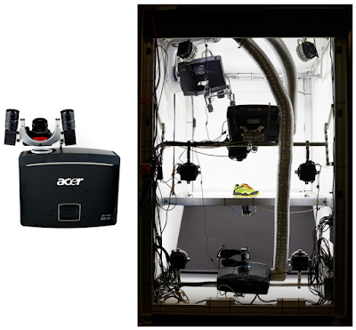
To create high-quality models, we built a scanning rig to capture images of an object from multiple directions under controlled and carefully calibrated conditions. The system consists of two machine vision cameras for shape detection, a DSLR camera for high-quality HDR color frame extraction, and a computer-controlled projector for pattern recognition. The scanning rig uses a structured light technique that infers a 3D shape from camera images with patterns of light that are projected onto an object.

The scanning rig used to capture 3D models.

A shoe being scanned (left). Images are captured from several directions with different patterns of light and color. A shadow passing over an object (right) illustrates how a 3D shape can be captured with an off-axis view of a shadow edge.

Simulation Model Conversion
The early internal scanned models used protocol buffer metadata, high-resolution visuals, and formats that were not suitable for simulation. For some objects, physical properties, such as mass, were captured by weighing the objects at scanning time, but surface properties, such as friction or deformation, were not represented.

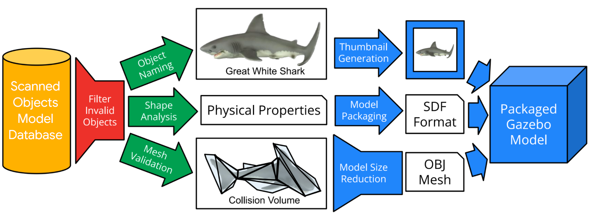
So, following data collection, we built an automated pipeline to solve these issues and enable the use of scanned models in simulation systems. The automated pipeline filters out invalid or duplicate objects, automatically assigns object names using text descriptions of the objects, and eliminates object mesh scans that do not meet simulation requirements. Next, the pipeline estimates simulation properties (e.g., mass and moment of inertia) from shape and volume, constructs collision volumes, and downscales the model to a usable size. Finally, the pipeline converts each model to SDF format, creates thumbnail images, and packages the model for use in simulation systems.

The pipeline filters models that are not suitable for simulation, generates collision volumes, computes physical properties, downsamples meshes, generates thumbnails, and packages them all for use in simulation systems.

A collection of Scanned Object models rendered in Blender.

The output of this pipeline is a simulation model in an appropriate format with a name, mass, friction, inertia, and collision information, along with searchable metadata in a public interface compatible with our open-source hosting on Open Robotics’ Gazebo.

The output objects are represented as SDF models that refer to Wavefront OBJ meshes averaging 1.4 Mb per model. Textures for these models are in PNG format and average 11.2 Mb. Together, these provide high resolution shape and texture.

Impact
The Scanned Objects dataset contains 1030 scanned objects and their associated metadata, totaling 13 Gb, licensed under the CC-BY 4.0 License. Because these models are scanned rather than modeled by hand, they realistically reflect real object properties, not idealized recreations, reducing the difficulty of transferring learning from simulation to the real world.

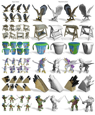
Input views (left) and reconstructed shape and texture from two novel views on the right (figure from Differentiable Stereopsis).

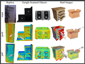
Visualized action scoring predictions over three real-world 3D scans from the Replica dataset and Scanned Objects (figure from Where2Act).

The Scanned Objects dataset has already been used in over 25 papers across as many projects, spanning computer vision, computer graphics, robot manipulation, robot navigation, and 3D shape processing. Most projects used the dataset to provide synthetic training data for learning algorithms. For example, the Scanned Objects dataset was used in Kubric, an open-sourced generator of scalable datasets for use in over a dozen vision tasks, and in LAX-RAY, a system for searching shelves with lateral access X-rays to automate the mechanical search for occluded objects on shelves.

Unsupervised 3D keypoints on real-world data (figure from KeypointDeformer).

We hope that the Scanned Objects dataset will be used by more robotics and simulation researchers in the future, and that the example set by this dataset will inspire other owners of 3D model repositories to make them available for researchers everywhere. If you would like to try it yourself, head to Gazebo and start browsing!

Acknowledgments
The authors thank the Scanned Objects team, including Peter Anderson-Sprecher, J.J. Blumenkranz, James Bruce, Ken Conley, Katie Dektar, Charles DuHadway, Anthony Francis, Chaitanya Gharpure, Topraj Gurung, Kristy Headley, Ryan Hickman, John Isidoro, Sumit Jain, Brandon Kinman, Greg Kline, Mach Kobayashi, Nate Koenig, Kai Kohlhoff, James Kuffner, Thor Lewis, Mike Licitra, Lexi Martin, Julian (Mac) Mason, Rus Maxham, Pascal Muetschard, Kannan Pashupathy, Barbara Petit, Arshan Poursohi, Jared Russell, Matt Seegmiller, John Sheu, Joe Taylor, Vincent Vanhoucke, Josh Weaver, and Tommy McHugh.

Special thanks go to Krista Reymann for organizing this project, helping write the paper, and editing this blogpost, James Bruce for the scanning pipeline design and Pascal Muetschard for maintaining the database of object models.

Source: Google AI Blog

Large-Scale Matrix Factorization on TPUs

Posted by Harsh Mehta, Software Engineer, Google Research

Matrix factorization is one of the oldest, yet still widely used, techniques for learning how to recommend items such as songs or movies from user ratings. In its basic form, it approximates a large, sparse (i.e., mostly empty) matrix of user-item interactions with a product of two smaller, denser matrices representing learned item and user features. These dense matrices, in turn, can be used to recommend items to a user with which they haven't interacted before.

Despite its algorithmic simplicity, matrix factorization can still achieve competitive performance in recommender benchmarks. Alternating least squares (ALS), and especially its implicit variation, is a fundamental algorithm to learn the parameters of matrix factorization. ALS is known for its high efficiency because it scales linearly in the number of rows, columns and non-zeros. Hence, this algorithm is very well suited for large-scale challenges. But, for very large real-world matrix factorization datasets, a single machine implementation would not suffice, and so, it would require a large distributed system. Most of the distributed implementations of matrix factorization that employ ALS leverage off-the-shelf CPU devices, and rightfully so, due to the inherently sparse nature of the problem (the input matrix is mostly empty).

On the other hand, recent success of deep learning, which has exhibited growing computational capacity, has spurred a new wave of research and progress on hardware accelerators such as Tensor Processing Units (TPUs). TPUs afford domain specific hardware speedups, especially for use cases like deep learning, which involves a large number of dense matrix multiplications. In particular, they allow significant speedups for traditional data-parallel workloads, such as training models with Stochastic Gradient Descent (SGD) in SPMD (single program multiple data) fashion. The SPMD approach has gained popularity in computations like training neural networks with gradient descent algorithms, and can be used for both data-parallel and model-parallel computations, where we distribute parameters of the model across available devices. Nevertheless, while TPUs have been enormously attractive for methods based on SGD, it is not immediately clear if a high performance implementation of ALS, which requires a large number of distributed sparse matrix multiplies, can be developed for a large-scale cluster of TPU devices.

In “ALX: Large Scale Matrix Factorization on TPUs”, we explore a distributed ALS design that makes efficient use of the TPU architecture and can scale well to matrix factorization problems of the order of billions of rows and columns by scaling the number of available TPU cores. The approach we propose leverages a combination of model and data parallelism, where each TPU core both stores a portion of the embedding table and trains over a unique slice of data, grouped in mini-batches. In order to spur future research on large-scale matrix factorization methods and to illustrate the scalability properties of our own implementation, we also built and released a real world web link prediction dataset called WebGraph.

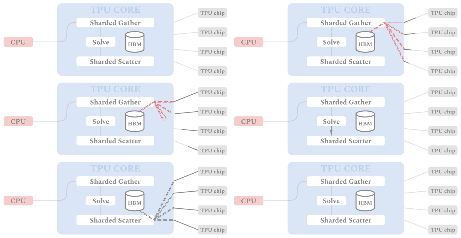
The figure shows the flow of data and computation through the ALX framework on TPU devices. Similar to SGD-based training procedures, each TPU core performs identical computation for its own batch of data in SPMD fashion, which allows for synchronous computation in parallel on multiple TPU cores. Each TPU starts with gathering all the relevant item embeddings in the Sharded Gather stage. These materialized embeddings are used to solve for user embeddings which are scattered to the relevant shard of the embedding table in the Sharded Scatter stage.

Dense Batching for Improved Efficiency
We designed ALX specifically for TPUs, exploiting unique properties of TPU architecture while overcoming a few interesting limitations. For instance, each TPU core has limited memory and restricts all tensors to have a static shape, but each example in a mini-batch can have a wildly varying number of items (i.e., inputs can be long and sparse). To resolve this, we break exceedingly long examples into multiple smaller examples of the same shape, a process called dense batching. More details about dense batching can be found in our paper.

Illustrating example of how sparse batches are densified to increase efficiency on TPUs.

Uniform Sharding of Embedding Tables
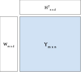
With the batching problem solved, we next want to factorize a sparse matrix into two dense embedding matrices (e.g., user and item embeddings) such that the resulting dot product of embeddings approximate the original sparse matrix — this helps us infer predictions for all the positions from the original matrix, including those that were empty, which can be used to recommend items with which users haven’t interacted. Both the resulting embedding tables (W and H in the figure below) can potentially be too large to fit in a single TPU core, thus requiring a distributed training setup for most large-scale use cases.

Most previous attempts of distributed matrix factorization use a parameter server architecture where the model parameters are stored on highly available servers, and the training data is processed in parallel by workers that are solely responsible for the learning task. In our case, since each TPU core has identical compute and memory, it's wasteful to only use either memory for storing model parameters or compute for training. Thus, we designed our system such that each core is used to do both.

Illustrative example of factorizing a sparse matrix Y into two dense embedding matrices W and H.

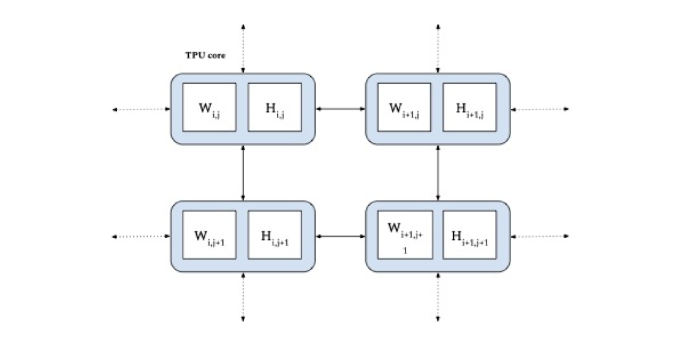
In ALX, we uniformly divide both embedding tables, thus fully exploiting both the size of distributed memory available and the dedicated low-latency interconnects between TPUs. This is highly efficient for very large embedding tables and results in good performance for distributed gather and scatter operations.

Uniform sharding of both embedding tables (W and H) across TPU cores (in blue).

WebGraph
Since potential applications may involve very large data sets, scalability is potentially an important opportunity for advancement in matrix factorization. To that end, we also release a large real-world web link prediction dataset called WebGraph. This dataset can be easily modeled as a matrix factorization problem where rows and columns are source and destination links, respectively, and the task is to predict destination links from each source link. We use WebGraph to illustrate the scaling properties of ALX.

The WebGraph dataset was generated from a single crawl performed by CommonCrawl in 2021 where we strip everything and keep only the link->outlinks data. Since the performance of a factorization method depends on the properties of the underlying graph, we created six versions of WebGraph, each varying in the sparsity pattern and locale, to study how well ALS performs on each.

To study locale-specific graphs, we filter based on two top level domains: ‘de’ and ‘in’, each producing a graph with an order of magnitude fewer nodes.
These graphs can still have arbitrary sparsity patterns and dangling links. Thus we further filter the nodes in each graph to have a minimum of either 10 or 50 inlinks and outlinks.

For easy access, we have made these available as a Tensorflow Dataset package. For reference, the biggest version, WebGraph-sparse, has more than 365M nodes and 30B edges. We create and publish both training and testing splits for evaluation purposes.

Results
We carefully tune the system and quality parameters of ALX. Based on our observations related to precision and choice of linear solvers. We observed that by carefully selecting the precision for storage of the embedding tables (bfloat16) and for the input to the linear solvers (float32), we were able to halve the memory required for the embeddings while still avoiding problems arising from lower precision values during the solve stage. For our linear solvers, we selected conjugate gradients, which we found to be the fastest across the board on TPUs. We use embeddings of dimension 128 and train the model for 16 epochs. In our experience, hyperparameter tuning over both norm penalty (λ) and unobserved weight (α) has been indispensable for good recall metrics as shown in the table below.

Results obtained by running ALX on all versions of WebGraph dataset. Recall values of 1.0 denote perfect recall.

Scaling Analysis
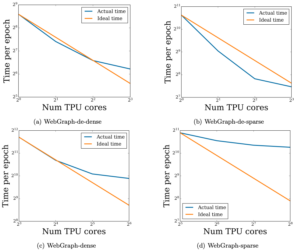
Since the input data are processed in parallel across TPU cores, increasing the number of cores decreases training time, ideally in a linear fashion. But at the same time, a larger number of cores requires more network communication (due to the sharded embedding tables). Thanks to high-speed interconnects, this overhead can be negligible for a small number of cores, but as the number of cores increases, the overhead eventually slows down the ideal linear scaling.

In order to confirm our hypothesis, we analyze scaling properties of the four biggest WebGraph variants in terms of training time as we increase the number of available TPU cores. As shown below, even empirically, we do observe the predicted linear decrease in training time up to a sweet spot, after which the network overhead slows the decline.

Scaling analysis of running time as the number of TPU cores are increased. Each figure plots the time taken to train for one epoch in seconds.

Conclusion
For easy access and reproducibility, the ALX code is open-sourced and can be easily run on Google Cloud. In fact, we illustrate that a sparse matrix like WebGraph-dense of size 135M x 135M (with 22B edges) can be factorized in a colab connected to 8 TPU cores in less than a day. We have designed the ALX framework with scalability in mind. With 256 TPU cores, one epoch of the largest WebGraph variant, WebGraph-sparse (365M x 365M sparse matrix) takes around 20 minutes to finish (5.5 hours for the whole training run). The final model has around 100B parameters. We hope that the ALX and WebGraph will be useful to both researchers and practitioners working in these fields. The code for ALX can be found here on github!

Acknowledgements
The core team includes Steffen Rendle, Walid Krichene and Li Zhang. We thank many Google colleagues for helping at various stages of this project. In particular, we are grateful to the JAX team for numerous discussions, especially James Bradbury and Skye Wanderman-Milne; Blake Hechtman for help with XLA and Rasmus Larsen for useful discussions about performance of linear solvers on TPUs. Finally, we're also grateful to Nicolas Mayoraz, John Anderson, and Fernando Pereira for providing useful feedback.

Source: Google AI Blog

Introducing CVSS: A Massively Multilingual Speech-to-Speech Translation Corpus

Posted by Ye Jia and Michelle Tadmor Ramanovich, Software Engineers, Google Research

Automatic translation of speech from one language to speech in another language, called speech-to-speech translation (S2ST), is important for breaking down the communication barriers between people speaking different languages. Conventionally, automatic S2ST systems are built with a cascade of automatic speech recognition (ASR), text-to-text machine translation (MT), and text-to-speech (TTS) synthesis sub-systems, so that the system overall is text-centric. Recently, work on S2ST that doesn’t rely on intermediate text representation is emerging, such as end-to-end direct S2ST (e.g., Translatotron) and cascade S2ST based on learned discrete representations of speech (e.g., Tjandra et al.). While early versions of such direct S2ST systems obtained lower translation quality compared to cascade S2ST models, they are gaining traction as they have the potential both to reduce translation latency and compounding errors, and to better preserve paralinguistic and non-linguistic information from the original speech, such as voice, emotion, tone, etc. However, such models usually have to be trained on datasets with paired S2ST data, but the public availability of such corpora is extremely limited.

To foster research on such a new generation of S2ST, we introduce a Common Voice-based Speech-to-Speech translation corpus, or CVSS, which includes sentence-level speech-to-speech translation pairs from 21 languages into English. Unlike existing public corpora, CVSS can be directly used for training such direct S2ST models without any extra processing. In “CVSS Corpus and Massively Multilingual Speech-to-Speech Translation”, we describe the dataset design and development, and demonstrate the effectiveness of the corpus through training of baseline direct and cascade S2ST models and showing performance of a direct S2ST model that approaches that of a cascade S2ST model.

Building CVSS
CVSS is directly derived from the CoVoST 2 speech-to-text (ST) translation corpus, which is further derived from the Common Voice speech corpus. Common Voice is a massively multilingual transcribed speech corpus designed for ASR in which the speech is collected by contributors reading text content from Wikipedia and other text corpora. CoVoST 2 further provides professional text translation for the original transcript from 21 languages into English and from English into 15 languages. CVSS builds on these efforts by providing sentence-level parallel speech-to-speech translation pairs from 21 languages into English (shown in the table below).

To facilitate research with different focuses, two versions of translation speech in English are provided in CVSS, both are synthesized using state-of-the-art TTS systems, with each version providing unique value that doesn’t exist in other public S2ST corpora:

CVSS-C: All the translation speech is in a single canonical speaker’s voice. Despite being synthetic, the speech is highly natural, clean, and consistent in speaking style. These properties ease the modeling of the target speech and enable trained models to produce high quality translation speech suitable for general user-facing applications where speech quality is of higher importance than accurately reproducing the speakers' voices.
CVSS-T: The translation speech captures the voice from the corresponding source speech. Each S2ST pair has a similar voice on the two sides, despite being in different languages. Because of this, the dataset is suitable for building models where accurate voice preservation is desired, such as for movie dubbing.

Together with the source speech, the two S2ST datasets contain 1,872 and 1,937 hours of speech, respectively.

Source Language	Code	Source speech (X)	CVSS-C target speech (En)	CVSS-T target speech (En)
French	fr	309.3	200.3	222.3
German	de	226.5	137.0	151.2
Catalan	ca	174.8	112.1	120.9
Spanish	es	157.6	94.3	100.2
Italian	it	73.9	46.5	49.2
Persian	fa	58.8	29.9	34.5
Russian	ru	38.7	26.9	27.4
Chinese	zh	26.5	20.5	22.1
Portuguese	pt	20.0	10.4	11.8
Dutch	nl	11.2	7.3	7.7
Estonian	et	9.0	7.3	7.1
Mongolian	mn	8.4	5.1	5.7
Turkish	tr	7.9	5.4	5.7
Arabic	ar	5.8	2.7	3.1
Latvian	lv	4.9	2.6	3.1
Swedish	sv	4.3	2.3	2.8
Welsh	cy	3.6	1.9	2.0
Tamil	ta	3.1	1.7	2.0
Indonesian	id	3.0	1.6	1.7
Japanese	ja	3.0	1.7	1.8
Slovenian	sl	2.9	1.6	1.9
Total		1,153.2	719.1	784.2

Amount of source and target speech of each X-En pair in CVSS (hours).

In addition to translation speech, CVSS also provides normalized translation text matching the pronunciation in the translation speech (on numbers, currencies, acronyms, etc., see data samples below, e.g., where “100%” is normalized as “one hundred percent” or “King George II” is normalized as “king george the second”), which can benefit both model training as well as standardizing the evaluation.

CVSS is released under the Creative Commons Attribution 4.0 International (CC BY 4.0) license and it can be freely downloaded online.

Data Samples

*Example 1:*
Source audio (French)

Source transcript (French)		Le genre musical de la chanson est entièrement le disco.

CVSS-C translation audio (English)
CVSS-T translation audio (English)

Translation text (English)		The musical genre of the song is 100% Disco.

Normalized translation text (English)		the musical genre of the song is one hundred percent disco


*Example 2:*
Source audio (Chinese)

Source transcript (Chinese)		弗雷德里克王子，英国王室成员，为乔治二世之孙，乔治三世之幼弟。

CVSS-C translation audio (English)
CVSS-T translation audio (English)

Translation text (English)		Prince Frederick, member of British Royal Family, Grandson of King George II, brother of King George III.

Normalized translation text (English)		prince frederick member of british royal family grandson of king george the second brother of king george the third

Baseline Models
On each version of CVSS, we trained a baseline cascade S2ST model as well as two baseline direct S2ST models and compared their performance. These baselines can be used for comparison in future research.

Cascade S2ST: To build strong cascade S2ST baselines, we trained an ST model on CoVoST 2, which outperforms the previous states of the art by +5.8 average BLEU on all 21 language pairs (detailed in the paper) when trained on the corpus without using extra data. This ST model is connected to the same TTS models used for constructing CVSS to compose very strong cascade S2ST baselines (ST → TTS).

Direct S2ST: We built two baseline direct S2ST models using Translatotron and Translatotron 2. When trained from scratch with CVSS, the translation quality from Translatotron 2 (8.7 BLEU) approaches that of the strong cascade S2ST baseline (10.6 BLEU). Moreover, when both use pre-training the gap decreases to only 0.7 BLEU on ASR transcribed translation. These results verify the effectiveness of using CVSS to train direct S2ST models.

Translation quality of baseline direct and cascade S2ST models built on CVSS-C, measured by BLEU on ASR transcription from speech translation. The pre-training was done on CoVoST 2 without other extra data sets.

Conclusion
We have released two versions of multilingual-to-English S2ST datasets, CVSS-C and CVSS-T, each with about 1.9K hours of sentence-level parallel S2ST pairs, covering 21 source languages. The translation speech in CVSS-C is in a single canonical speaker’s voice, while the same in CVSS-T is in voices transferred from the source speech. Each of these datasets provides unique value not existing in other public S2ST corpora.

We built baseline multilingual direct S2ST models and cascade S2ST models on both datasets, which can be used for comparison in future works. To build strong cascade S2ST baselines, we trained an ST model on CoVoST 2, which outperforms the previous states of the art by +5.8 average BLEU when trained on the corpus without extra data. Nevertheless, the performance of the direct S2ST models approaches the strong cascade baselines when trained from scratch, and with only 0.7 BLEU difference on ASR transcribed translation when utilized pre-training. We hope this work helps accelerate the research on direct S2ST.

Acknowledgments
We acknowledge the volunteer contributors and the organizers of the Common Voice and LibriVox projects for their contribution and collection of recordings, the creators of Common Voice, CoVoST, CoVoST 2, Librispeech and LibriTTS corpora for their previous work. The direct contributors to the CVSS corpus and the paper include Ye Jia, Michelle Tadmor Ramanovich, Quan Wang, Heiga Zen. We also thank Ankur Bapna, Yiling Huang, Jason Pelecanos, Colin Cherry, Alexis Conneau, Yonghui Wu, Hadar Shemtov and Françoise Beaufays for helpful discussions and support.

googblogs.com

All Google blogs and Press in one site

Tag Archives: datasets

The Data Cards Playbook: A Toolkit for Transparency in Dataset Documentation

The Data Cards Playbook

Activities, Foundations, and Transparency Patterns

Playbook Modules

In Practice

Conclusion

Acknowledgements

Source: Google AI Blog

Open Images V7 — Now Featuring Point Labels

Point Labels

New Visualizers

Conclusion

Acknowledgements

Source: Google AI Blog

Crossmodal-3600 — Multilingual Reference Captions for Geographically Diverse Images

Source: Google AI Blog

Announcing the Patent Phrase Similarity Dataset

Source: Google AI Blog

UVQ: Measuring YouTube’s Perceptual Video Quality

Source: Google AI Blog

UVQ: Measuring YouTube’s Perceptual Video Quality

Source: Google AI Blog

Scanned Objects by Google Research: A Dataset of 3D-Scanned Common Household Items

Source: Google AI Blog

Large-Scale Matrix Factorization on TPUs

Source: Google AI Blog

Introducing CVSS: A Massively Multilingual Speech-to-Speech Translation Corpus

Source: Google AI Blog