Tag Archives: open source release

DeepVariant: Highly Accurate Genomes With Deep Neural Networks

Crossposted on the Google Research Blog

Across many scientific disciplines, but in particular in the field of genomics, major breakthroughs have often resulted from new technologies. From Sanger sequencing, which made it possible to sequence the human genome, to the microarray technologies that enabled the first large-scale genome-wide experiments, new instruments and tools have allowed us to look ever more deeply into the genome and apply the results broadly to health, agriculture and ecology.

One of the most transformative new technologies in genomics was high-throughput sequencing (HTS), which first became commercially available in the early 2000s. HTS allowed scientists and clinicians to produce sequencing data quickly, cheaply, and at scale. However, the output of HTS instruments is not the genome sequence for the individual being analyzed — for humans this is 3 billion paired bases (guanine, cytosine, adenine and thymine) organized into 23 pairs of chromosomes. Instead, these instruments generate ~1 billion short sequences, known as reads. Each read represents just 100 of the 3 billion bases, and per-base error rates range from 0.1-10%. Processing the HTS output into a single, accurate and complete genome sequence is a major outstanding challenge. The importance of this problem, for biomedical applications in particular, has motivated efforts such as the Genome in a Bottle Consortium (GIAB), which produces high confidence human reference genomes that can be used for validation and benchmarking, as well as the precisionFDA community challenges, which are designed to foster innovation that will improve the quality and accuracy of HTS-based genomic tests.

CAPTION: For any given location in the genome, there are multiple reads among the ~1 billion that include a base at that position. Each read is aligned to a reference, and then each of the bases in the read is compared to the base of the reference at that location. When a read includes a base that differs from the reference, it may indicate a variant (a difference in the true sequence), or it may be an error.

Today, we announce the open source release of DeepVariant, a deep learning technology to reconstruct the true genome sequence from HTS sequencer data with significantly greater accuracy than previous classical methods. This work is the product of more than two years of research by the Google Brain team, in collaboration with Verily Life Sciences. DeepVariant transforms the task of variant calling, as this reconstruction problem is known in genomics, into an image classification problem well-suited to Google's existing technology and expertise.

CAPTION: Each of the four images above is a visualization of actual sequencer reads aligned to a reference genome. A key question is how to use the reads to determine whether there is a variant on both chromosomes, on just one chromosome, or on neither chromosome. There is more than one type of variant, with SNPs and insertions/deletions being the most common. A: a true SNP on one chromosome pair, B: a deletion on one chromosome, C: a deletion on both chromosomes, D: a false variant caused by errors. It's easy to see that these look quite distinct when visualized in this manner.

We started with GIAB reference genomes, for which there is high-quality ground truth (or the closest approximation currently possible). Using multiple replicates of these genomes, we produced tens of millions of training examples in the form of multi-channel tensors encoding the HTS instrument data, and then trained a TensorFlow-based image classification model to identify the true genome sequence from the experimental data produced by the instruments. Although the resulting deep learning model, DeepVariant, had no specialized knowledge about genomics or HTS, within a year it had won the the highest SNP accuracy award at the precisionFDA Truth Challenge, outperforming state-of-the-art methods. Since then, we've further reduced the error rate by more than 50%.


DeepVariant is being released as open source software to encourage collaboration and to accelerate the use of this technology to solve real world problems. To further this goal, we partnered with Google Cloud Platform (GCP) to deploy DeepVariant workflows on GCP, available today, in configurations optimized for low-cost and fast turnarounds using scalable GCP technologies like the Pipelines API. This paired set of releases provides a smooth ramp for users to explore and evaluate the capabilities of DeepVariant in their current compute environment while providing a scalable, cloud-based solution to satisfy the needs of even the largest genomics datasets.

DeepVariant is the first of what we hope will be many contributions that leverage Google's computing infrastructure and ML expertise to both better understand the genome and to provide deep learning-based genomics tools to the community. This is all part of a broader goal to apply Google technologies to healthcare and other scientific applications, and to make the results of these efforts broadly accessible.

By Mark DePristo and Ryan Poplin, Google Brain Team

Tangent: Source-to-Source Debuggable Derivatives

Crossposted on the Google Research Blog

Tangent is a new, free, and open source Python library for automatic differentiation. In contrast to existing machine learning libraries, Tangent is a source-to-source system, consuming a Python function f and emitting a new Python function that computes the gradient of f. This allows much better user visibility into gradient computations, as well as easy user-level editing and debugging of gradients. Tangent comes with many more features for debugging and designing machine learning models.
This post gives an overview of the Tangent API. It covers how to use Tangent to generate gradient code in Python that is easy to interpret, debug and modify.

Neural networks (NNs) have led to great advances in machine learning models for images, video, audio, and text. The fundamental abstraction that lets us train NNs to perform well at these tasks is a 30-year-old idea called reverse-mode automatic differentiation (also known as backpropagation), which comprises two passes through the NN. First, we run a “forward pass” to calculate the output value of each node. Then we run a “backward pass” to calculate a series of derivatives to determine how to update the weights to increase the model’s accuracy.

Training NNs, and doing research on novel architectures, requires us to compute these derivatives correctly, efficiently, and easily. We also need to be able to debug these derivatives when our model isn’t training well, or when we’re trying to build something new that we do not yet understand. Automatic differentiation, or just “autodiff,” is a technique to calculate the derivatives of computer programs that denote some mathematical function, and nearly every machine learning library implements it.

Existing libraries implement automatic differentiation by tracing a program’s execution (at runtime, like TF Eager, PyTorch and Autograd) or by building a dynamic data-flow graph and then differentiating the graph (ahead-of-time, like TensorFlow). In contrast, Tangent performs ahead-of-time autodiff on the Python source code itself, and produces Python source code as its output.
As a result, you can finally read your automatic derivative code just like the rest of your program. Tangent is useful to researchers and students who not only want to write their models in Python, but also read and debug automatically-generated derivative code without sacrificing speed and flexibility.

You can easily inspect and debug your models written in Tangent, without special tools or indirection. Tangent works on a large and growing subset of Python, provides extra autodiff features other Python ML libraries don’t have, is high-performance, and is compatible with TensorFlow and NumPy.

Automatic differentiation of Python code

How do we automatically generate derivatives of plain Python code? Math functions like tf.exp or tf.log have derivatives, which we can compose to build the backward pass. Similarly, pieces of syntax, such as  subroutines, conditionals, and loops, also have backward-pass versions. Tangent contains recipes for generating derivative code for each piece of Python syntax, along with many NumPy and TensorFlow function calls.

Tangent has a one-function API:
import tangent
df = tangent.grad(f)
Here’s an animated graphic of what happens when we call tangent.grad on a Python function:
If you want to print out your derivatives, you can run
import tangent
df = tangent.grad(f, verbose=1)
Under the hood, tangent.grad first grabs the source code of the Python function you pass it. Tangent has a large library of recipes for the derivatives of Python syntax, as well as TensorFlow Eager functions. The function tangent.grad then walks your code in reverse order, looks up the matching backward-pass recipe, and adds it to the end of the derivative function. This reverse-order processing gives the technique its name: reverse-mode automatic differentiation.

The function df above only works for scalar (non-array) inputs. Tangent also supports
Although we started with TensorFlow Eager support, Tangent isn’t tied to one numeric library or another—we would gladly welcome pull requests adding PyTorch or MXNet derivative recipes.

Next Steps

Tangent is open source now at github.com/google/tangent. Go check it out for download and installation instructions. Tangent is still an experiment, so expect some bugs. If you report them to us on GitHub, we will do our best to fix them quickly.

We are working to add support in Tangent for more aspects of the Python language (e.g., closures, inline function definitions, classes, more NumPy and TensorFlow functions). We also hope to add more advanced automatic differentiation and compiler functionality in the future, such as automatic trade-off between memory and compute (Griewank and Walther 2000; Gruslys et al., 2016), more aggressive optimizations, and lambda lifting.

We intend to develop Tangent together as a community. We welcome pull requests with fixes and features. Happy deriving!

By Alex Wiltschko, Research Scientist, Google Brain Team

Acknowledgments

Bart van Merriënboer contributed immensely to all aspects of Tangent during his internship, and Dan Moldovan led TF Eager integration, infrastructure and benchmarking. Also, thanks to the Google Brain team for their support of this post and special thanks to Sanders Kleinfeld and Aleks Haecky for their valuable contribution for the technical aspects of the post.

Announcing OpenFermion: The Open Source Chemistry Package for Quantum Computers

Crossposted on the Google Research Blog

“The underlying physical laws necessary for the mathematical theory of a large part of physics and the whole of chemistry are thus completely known, and the difficulty is only that the exact application of these laws leads to equations much too complicated to be soluble.”
-Paul Dirac, Quantum Mechanics of Many-Electron Systems (1929)

In this passage, physicist Paul Dirac laments that while quantum mechanics accurately models all of chemistry, exactly simulating the associated equations appears intractably complicated. Not until 1982 would Richard Feynman suggest that instead of surrendering to the complexity of quantum mechanics, we might harness it as a computational resource. Hence, the original motivation for quantum computing: by operating a computer according to the laws of quantum mechanics, one could efficiently unravel exact simulations of nature. Such simulations could lead to breakthroughs in areas such as photovoltaics, batteries, new materials, pharmaceuticals and superconductivity. And while we do not yet have a quantum computer large enough to solve classically intractable problems in these areas, rapid progress is being made. Last year, Google published this paper detailing the first quantum computation of a molecule using a superconducting qubit quantum computer. Building on that work, the quantum computing group at IBM scaled the experiment to larger molecules, which made the cover of Nature last month.

Today, we announce the release of OpenFermion, the first open source platform for translating problems in chemistry and materials science into quantum circuits that can be executed on existing platforms. OpenFermion is a library for simulating the systems of interacting electrons (fermions) which give rise to the properties of matter. Prior to OpenFermion, quantum algorithm developers would need to learn a significant amount of chemistry and write a large amount of code hacking apart other codes to put together even the most basic quantum simulations. While the project began at Google, collaborators at ETH Zurich, Lawrence Berkeley National Labs, University of Michigan, Harvard University, Oxford University, Dartmouth College, Rigetti Computing and NASA all contributed to alpha releases. You can learn more details about this release in our paper, OpenFermion: The Electronic Structure Package for Quantum Computers.

One way to think of OpenFermion is as a tool for generating and compiling physics equations which describe chemical and material systems into representations which can be interpreted by a quantum computer1. The most effective quantum algorithms for these problems build upon and extend the power of classical quantum chemistry packages used and developed by research chemists across government, industry and academia. Accordingly, we are also releasing OpenFermion-Psi4 and OpenFermion-PySCF which are plugins for using OpenFermion in conjunction with the classical electronic structure packages Psi4 and PySCF.

The core OpenFermion library is designed in a quantum programming framework agnostic way to ensure compatibility with various platforms being developed by the community. This allows OpenFermion to support external packages which compile quantum assembly language specifications for diverse hardware platforms. We hope this decision will help establish OpenFermion as a community standard for putting quantum chemistry on quantum computers. To see how OpenFermion is used with diverse quantum programming frameworks, take a look at OpenFermion-ProjectQ and Forest-OpenFermion - plugins which link OpenFermion to the externally developed circuit simulation and compilation platforms known as ProjectQ and Forest.

The following workflow describes how a quantum chemist might use OpenFermion in order to simulate the energy surface of a molecule (for instance, by preparing the sort of quantum computation we described in our past blog post):
  1. The researcher initializes an OpenFermion calculation with specification of:
    • An input file specifying the coordinates of the nuclei in the molecule.
    • The basis set (e.g. cc-pVTZ) that should be used to discretize the molecule.
    • The charge and spin multiplicity (if known) of the system.
  1. The researcher uses the OpenFermion-Psi4 plugin or the OpenFermion-PySCF plugin to perform scalable classical computations which are used to optimally stage the quantum computation. For instance, one might perform a classical Hartree-Fock calculation to choose a good initial state for the quantum simulation.
  2. The researcher then specifies which electrons are most interesting to study on a quantum computer (known as an active space) and asks OpenFermion to map the equations for those electrons to a representation suitable for quantum bits, using one of the available procedures in OpenFermion, e.g. the Bravyi-Kitaev transformation.
  3. The researcher selects a quantum algorithm to solve for the properties of interest and uses a quantum compilation framework such as OpenFermion-ProjectQ to output the quantum circuit in assembly language which can be run on a quantum computer. If the researcher has access to a quantum computer, they then execute the experiment.
A few examples of what one might do with OpenFermion are demonstrated in ipython notebooks here, here and here. While quantum simulation is widely recognized as one of the most important applications of quantum computing in the near term, very few quantum computer scientists know quantum chemistry and even fewer chemists know quantum computing. Our hope is that OpenFermion will help to close the gap between these communities and bring the power of quantum computing to chemists and material scientists. If you’re interested, please checkout our GitHub repository - pull requests welcome! By Ryan Babbush and Jarrod McClean, Quantum Software Engineers, Quantum AI Team

1 If we may be allowed one sentence for the experts: the primary function of OpenFermion is to encode the electronic structure problem in second quantization defined by various basis sets and active spaces and then to transform those operators into spin Hamiltonians using various isomorphisms between qubit and fermion algebras.

TensorFlow Lattice: Flexibility Empowered by Prior Knowledge

Crossposted on the Google Research Blog

Machine learning has made huge advances in many applications including natural language processing, computer vision and recommendation systems by capturing complex input/output relationships using highly flexible models. However, a remaining challenge is problems with semantically meaningful inputs that obey known global relationships, like “the estimated time to drive a road goes up if traffic is heavier, and all else is the same.” Flexible models like DNNs and random forests may not learn these relationships, and then may fail to generalize well to examples drawn from a different sampling distribution than the examples the model was trained on.

Today we present TensorFlow Lattice, a set of prebuilt TensorFlow Estimators that are easy to use, and TensorFlow operators to build your own lattice models. Lattices are multi-dimensional interpolated look-up tables (for more details, see [1--5]), similar to the look-up tables in the back of a geometry textbook that approximate a sine function.  We take advantage of the look-up table’s structure, which can be keyed by multiple inputs to approximate an arbitrarily flexible relationship, to satisfy monotonic relationships that you specify in order to generalize better. That is, the look-up table values are trained to minimize the loss on the training examples, but in addition, adjacent values in the look-up table are constrained to increase along given directions of the input space, which makes the model outputs increase in those directions. Importantly, because they interpolate between the look-up table values, the lattice models are smooth and the predictions are bounded, which helps to avoid spurious large or small predictions in the testing time.

How Lattice Models Help You

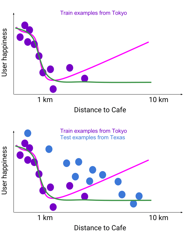
Suppose you are designing a system to recommend nearby coffee shops to a user. You would like the model to learn, “if two cafes are the same, prefer the closer one.”  Below we show a flexible model (pink) that accurately fits some training data for users in Tokyo (purple), where there are many coffee shops nearby.  The pink flexible model overfits the noisy training examples, and misses the overall trend that a closer cafe is better. If you used this pink model to rank test examples from Texas (blue), where businesses are spread farther out, you would find it acted strangely, sometimes preferring farther cafes!
Slice through a model’s feature space where all the other inputs stay the same and only distance changes. A flexible function (pink) that is accurate on training examples from Tokyo (purple) predicts that a cafe 10km-away is better than the same cafe if it was 5km-away. This problem becomes more evident at test-time if the data distribution has shifted, as shown here with blue examples from Texas where cafes are spread out more.
A monotonic flexible function (green) is both accurate on training examples and can generalize for Texas examples compared to non-monotonic flexible function (pink) from the previous figure.

In contrast, a lattice model, trained over the same example from Tokyo, can be constrained to satisfy such a monotonic relationship and result in a monotonic flexible function (green). The green line also accurately fits the Tokyo training examples, but also generalizes well to Texas, never preferring farther cafes.

In general, you might have many inputs about each cafe, e.g., coffee quality, price, etc. Flexible models have a hard time capturing global relationships of the form, “if all other inputs are equal, nearer is better, ” especially in parts of the feature space where your training data is sparse and noisy. Machine learning models that capture prior knowledge (e.g.  how inputs should impact the prediction) work better in practice, and are easier to debug and more interpretable.

Pre-built Estimators

We provide a range of lattice model architectures as TensorFlow Estimators. The simplest estimator we provide is the calibrated linear model, which learns the best 1-d transformation of each feature (using 1-d lattices), and then combines all the calibrated features linearly. This works well if the training dataset is very small, or there are no complex nonlinear input interactions. Another estimator is a calibrated lattice model. This model combines the calibrated features nonlinearly using a two-layer single lattice model, which can represent complex nonlinear interactions in your dataset. The calibrated lattice model is usually a good choice if you have 2-10 features, but for 10 or more features, we expect you will get the best results with an ensemble of calibrated lattices, which you can train using the pre-built ensemble architectures. Monotonic lattice ensembles can achieve 0.3% -- 0.5% accuracy gain compared to Random Forests [4], and these new TensorFlow lattice estimators can achieve 0.1 -- 0.4% accuracy gain compared to the prior state-of-the-art in learning models with monotonicity [5].

Build Your Own

You may want to experiment with deeper lattice networks or research using partial monotonic functions as part of a deep neural network or other TensorFlow architecture. We provide the building blocks: TensorFlow operators for calibrators, lattice interpolation, and monotonicity projections. For example, the figure below shows a 9-layer deep lattice network [5].


Example of a 9-layer deep lattice network architecture [5], alternating layers of linear embeddings and ensembles of lattices with calibrators layers (which act like a sum of ReLU’s in Neural Networks). The blue lines correspond to monotonic inputs, which is preserved layer-by-layer, and hence for the entire model. This and other arbitrary architectures can be constructed with TensorFlow Lattice because each layer is differentiable.

In addition to the choice of model flexibility and standard L1 and L2 regularization, we offer new regularizers with TensorFlow Lattice:
  • Monotonicity constraints [3] on your choice of inputs as described above.
  • Laplacian regularization [3] on the lattices to make the learned function flatter.
  • Torsion regularization [3] to suppress un-necessary nonlinear feature interactions.
We hope TensorFlow Lattice will be useful to the larger community working with meaningful semantic inputs. This is part of a larger research effort on interpretability and controlling machine learning models to satisfy policy goals, and enable practitioners to take advantage of their prior knowledge. We’re excited to share this with all of you. To get started, please check out our GitHub repository and our tutorials, and let us know what you think!

By Maya Gupta, Research Scientist, Jan Pfeifer, Software Engineer and Seungil You, Software Engineer

Acknowledgements

Developing and open sourcing TensorFlow Lattice was a huge team effort. We’d like to thank all the people involved: Andrew Cotter, Kevin Canini, David Ding, Mahdi Milani Fard, Yifei Feng, Josh Gordon, Kiril Gorovoy, Clemens Mewald, Taman Narayan, Alexandre Passos, Christine Robson, Serena Wang, Martin Wicke, Jarek Wilkiewicz, Sen Zhao, Tao Zhu

References

[1] Lattice Regression, Eric Garcia, Maya Gupta, Advances in Neural Information Processing Systems (NIPS), 2009
[2] Optimized Regression for Efficient Function Evaluation, Eric Garcia, Raman Arora, Maya R. Gupta, IEEE Transactions on Image Processing, 2012
[3] Monotonic Calibrated Interpolated Look-Up Tables, Maya Gupta, Andrew Cotter, Jan Pfeifer, Konstantin Voevodski, Kevin Canini, Alexander Mangylov, Wojciech Moczydlowski, Alexander van Esbroeck, Journal of Machine Learning Research (JMLR), 2016
[4] Fast and Flexible Monotonic Functions with Ensembles of Lattices, Mahdi Milani Fard, Kevin Canini, Andrew Cotter, Jan Pfeifer, Maya Gupta, Advances in Neural Information Processing Systems (NIPS), 2016
[5] Deep Lattice Networks and Partial Monotonic Functions, Seungil You, David Ding, Kevin Canini, Jan Pfeifer, Maya R. Gupta, Advances in Neural Information Processing Systems (NIPS), 2017

Introducing Abseil, a new common libraries project

Today we are open sourcing Abseil, a collection of libraries drawn from the most fundamental pieces of Google’s internal codebase. These libraries are the nuts-and-bolts that underpin almost everything that Google runs. Bits and pieces of these APIs are embedded in most of our open source projects, and now we have brought them together into one comprehensive project. Abseil encompasses the most basic building blocks of Google’s codebase: code that is production tested and will be fully maintained for years to come.

Our C++ code repository is available at: https://github.com/abseil/abseil-cpp

By adopting these new Apache-licensed libraries, you can reap the benefit of years (over a decade in many cases) of our design and optimization work in this space. Our past experience is baked in.

Just as interesting, we’ve also prepared for the future: several types in Abseil’s C++ libraries are “pre-adoption” versions of C++17 types like string_view and optional - implemented in C++11 to the greatest extent possible. We look forward to moving more and more of our code to match the current standard, and using these new vocabulary types helps us make that transition. Importantly, in C++17 mode these types are merely aliases to the standard, ensuring that you only ever have one type for optional or string_view in a project at a time. Put another way: Abseil is focused on the engineering task of providing APIs that remain stable over time.

Consisting of the foundational C++ and Python code at Google, Abseil includes libraries that will grow to underpin other Google-backed open source projects like gRPC, Protobuf and TensorFlow. We love those projects, and we love the users of those projects - we want to ensure smooth usage for these things over time. In the next few months we’ll introduce new distribution methods to incorporate these projects as a collection into your project.

Continuing with the “over time” theme, Abseil aims for compatibility with major compilers, platforms and standard libraries for approximately 5 years. Our 5-year target also applies to language version: we assume everyone builds with C++11 at this point. (In 2019 we’ll start talking about requiring C++14 as our base language version.) This 5-year horizon is part of our balance between “support everything” and “provide modern implementations and APIs.”

Highlights of the initial release include:
  • Zero configuration: most platforms (OS, compiler, architecture) should just work.
  • Pre-adoption for C++17 types: string_view, optional, any. We’ll follow up with variant soon.
  • Our primary synchronization type, absl::Mutex, has an elegant interface and has been extensively optimized.
  • Efficient support for handling time: absl::Time and absl::Duration are conceptually similar to std::chrono types, but are concrete (not class templates) and have defined behavior in all cases. Additionally, our clock-sampling API absl::Now() is more heavily optimized than most standard library calls for std::chrono::system_clock::now().
  • String handling routines: among internal users, we’ve been told that releasing absl::StrCat(), absl::StrJoin(), and absl::StrSplit() would itself be a big improvement for the open source C++ world.
The project has support for C++ and some Python. Over time we’ll tie those two projects together more closely with shared logging and command-line flag infrastructure. To start contributing, please see our contribution guidelines and fork us on GitHub. Check out our documentation and community page for information on how to contact us, ask questions or contribute to Abseil.

By Titus Winters, Abseil Lead

Making the Google Developers Documentation Style Guide Public

Cross-posted on the Google Developers Blog

You can now use our developer-documentation style guide for open source documentation projects.

For some years now, our technical writers at Google have used an internal-only editorial style guide for most of our developer documentation. In order to better support external contributors to our open source projects, such as Kubernetes, AMP, or Dart, and to allow for more consistency across developer documentation, we're now making that style guide public.

If you contribute documentation to projects like those, you now have direct access to useful guidance about voice, tone, word choice, and other style considerations. It can be useful for general issues, like reminders to use second person, present tense, active voice, and the serial comma; it can also be great for checking very specific issues, like whether to write "app" or "application" when you want to be consistent with the Google Developers style.

The style guide is a reference document, so instead of reading through it in linear order, you can use it to look things up as needed. For matters of punctuation, grammar, and formatting, you can do a search-in-page to find items like "Commas," "Lists," and "Link text" in the left nav. For specific terms and phrases, you can look at the word list.

Keep an eye on the guide's release notes page for updates and developments, and send us your comments and suggestions via the Send Feedback link on each page of the guide—we want to hear from you as we continue to evolve the style guide.

Posted by Jed Hartman, Technical Writer

Bringing Real-time Spatial Audio to the Web with Songbird

For a virtual scene to be truly immersive, stunning visuals need to be accompanied by true spatial audio to create a realistic and believable experience. Spatial audio tools allow developers to include sounds that can come from any direction, and that are associated in 3D space with audio sources, thus completely enveloping the user in 360-degree sound.

Spatial audio helps draw the user into a scene and creates the illusion of entering an entirely new world. To make this possible, the Chrome Media team has created Songbird, an open source, spatial audio encoding engine that works in any web browser by using the Web Audio API.

The Songbird library takes in any number of mono audio streams and allows developers to programmatically place them in 3D space around the user. Songbird allows you to create immersive soundscapes, realistically reproducing reflection and reverb for the space you describe. Sounds bounce off walls and reflect off materials just as they would in real-life, capturing truly 360-degree sound. Songbird creates an ambisonic soundfield that can then be rendered in real-time for use in your application. We’ve partnered with the Omnitone project, which we blogged about last year, to add higher-order ambisonic support to Omnitone’s binaural renderer to produce far more accurate sounding audio than ever before.

Songbird encapsulates Omnitone and with it, developers can now add interactive, full-sphere audio to any web based application. Songbird can scale to any order ambisonics, thereby creating a more realistic sound and higher performance than what is achievable through standard Web Audio API.
Songbird Audio Processing Diagram
The implementation of Songbird is based on the Google spatial media specification. It expects mono input and outputs ambisonic (multichannel) ACN channel layout with SN3D normalization. Detailed documentation may be found here.

As the web emerges as an important VR platform for delivering content, spatial audio will play a vital role in users’ embrace of this new medium. Songbird and Omnitone are key tools in enabling spatial audio on the web platform and establishing it as a preeminent platform for compelling VR experiences. Combining these audio experiences with 3D JavaScript libraries like three.js gives a glimpse into the future on the web.
Demo combining spatial sound in 3D environment
This project was made possible through close collaboration with Google’s Daydream and Web Audio teams. This collaboration allowed us to deliver similar audio capabilities to the web as are available to developers creating Daydream applications.

We look forward to seeing what people do with Songbird now that it's open source. Check out the code on GitHub and let us know what you think. Also available are a number of demos on creating full spherical audio with Songbird.

By Jamieson Brettle and Drew Allen, Chrome Media Team

Authenticating to HashiCorp Vault using Google Cloud IAM

Applications often require access to small pieces of sensitive data at build or run time, referred to as secrets. Secrets are generally more sensitive than other environment variables or parts of your repository as they may grant access to additional data, such as user data.

HashiCorp Vault is a popular open source tool for secret management, which allows a developer to store, manage and control access to tokens, passwords, certificates, API keys and other secrets. Vault has many options for authentication, called authentication backends. These allow developers to use many kinds of identities to access Vault, including tokens, or usernames and passwords. As the number of developers on a team grows, these kinds of authentication options become impractical; and in enterprise scenarios, managing and auditing these identities becomes burdensome.

Today, we are pleased to announce a Google Cloud Platform IAM authentication backend for Vault. This allows a developer to use an existing IAM identity to authenticate to Vault. Using a service account, you can sign a JWT to show it came from a particular account, and use that to authenticate to Vault. Learn more in the documentation.


The following example in Go shows how a user can authenticate with Vault using this backend. This example assumes the Vault server has already been mounted at auth/gcp and configured.
package main

import (
...
vaultapi "github.com/hashicorp/vault/api"
"golang.org/x/oauth2"
"golang.org/x/oauth2/google"
"google.golang.org/api/iam/v1"
...
)

func main() {
// Start [PARAMS]
project := "project-123456"
serviceAccount := "[email protected]"
credsPath := "path/to/creds.json"

os.Setenv("VAULT_ADDR", "https://vault.mycompany.com")
defer os.Setenv("VAULT_ADDR", "")
// End [PARAMS]

// Start [GCP IAM Setup]
jsonBytes, err := ioutil.ReadFile(credsPath)
if err != nil {
log.Fatal(err)
}
config, err := google.JWTConfigFromJSON(jsonBytes, iam.CloudPlatformScope)
if err != nil {
log.Fatal(err)
}

httpClient := config.Client(oauth2.NoContext)
iamClient, err := iam.New(httpClient)
if err != nil {
log.Fatal(err)
}
// End [GCP IAM Setup]

// 1. Generate signed JWT using IAM.
resourceName := fmt.Sprintf("projects/%s/serviceAccounts/%s", project, serviceAccount)
jwtPayload := map[string]interface{}{
"aud": "auth/gcp/login",
"sub": serviceAccount,
"exp": time.Now().Add(time.Minute * 10).Unix(),
}

payloadBytes, err := json.Marshal(jwtPayload)
if err != nil {
log.Fatal(err)
}
signJwtReq := &iam.SignJwtRequest{
Payload: string(payloadBytes),
}

resp, err := iamClient.Projects.ServiceAccounts.SignJwt(
resourceName, signJwtReq).Do()
if err != nil {
log.Fatal(err)
}

// 2. Send signed JWT in login request to Vault.
vaultClient, err := vaultapi.NewClient(vaultapi.DefaultConfig())
if err != nil {
log.Fatal(err)
}

vaultResp, err := vaultClient.Logical().Write(
"auth/gcp/login",
map[string]interface{}{
"role": "test",
"jwt": resp.SignedJwt,
})

if err != nil {
log.Fatal(err)
}

// 3. Use auth token from response.
log.Println("Access token %s", vaultResp.Auth.ClientToken)
vaultClient.SetToken(vaultResp.Auth.ClientToken)
// ...
}

Vault is just one way of managing secrets in development. For further reading on choosing a solution that’s right for you, see Google Cloud Platform’s documentation on Secret Management.

By Emily Ye, Software Engineer

Making Great Mobile Games with Firebase

So much goes into building and maintaining a mobile game. Let’s say you want to ship it with a level builder for sharing content with other players and, looking forward, you want to roll out new content and unlockables linked with player behavior. Of course, you also need players to be able to easily sign into your soon-to-be hit game.

With a DIY approach, you’d be faced with having to build user management, data storage, server side logic, and more. This will take a lot of your time, and importantly, it would take critical resources away from what you really want to do: build that amazing new mobile game!

Our Firebase SDKs for Unity and C++ provide you with the tools you need to add these features and more to your game with ease. Plus, to help you better understand how Firebase can help you build your next chart-topper, we’ve built a sample game in Unity and open sourced it: MechaHamster. Check it out on Google Play or download the project from GitHub to see how easy it is to integrate Firebase into your game.
Before you dive into the code for Mecha Hamster, here’s a rundown of the Firebase products that can help your game be successful.

Analytics

One of the best tools you have to maintain a high-performing game is your analytics. With Google Analytics for Firebase, you can see where your players might be struggling and make adjustments as needed. Analytics also integrates with Adwords and other major ad networks to maximize your campaign performance. If you monetize your game using AdMob, you can link your two accounts and see the lifetime value (LTV) of your players, from in-game purchases and AdMob, right from your Analytics console. And with Streamview, you can see how players are interacting with your game in realtime.

Test Lab for Android - Game Loop Test

Before releasing updates to your game, you’ll want to make sure it works correctly. However, manual testing can be time consuming when faced with a large variety of target devices. To help solve this, we recently launched Firebase Test Lab for Android Game Loop Test at Google I/O. If you add a demo mode to your game, Test Lab will automatically verify your game is working on a wide range of devices. You can read more in our deep dive blog post here.

Authentication

Another thing you’ll want to be sure to take care of before launch is easy sign-in, so your users can start playing as quickly as possible. Firebase Authentication can help by handling all sign-in and authentication, from simple email + password logins to support for common identity providers like Google, Facebook, Twitter, and Github. Just announced recently at I/O, Firebase also now supports phone number authentication. And Firebase Authentication shares state cross-device, so your users can pick up where they left off, no matter what platforms they’re using.

Remote Config

As more players start using your game, you realize that there are few spots that are frustrating for your audience. You may even see churn rates start to rise, so you decide that you need to push some adjustments. With Firebase Remote Config, you can change values in the console and push them out to players. Some players having trouble navigating levels? You can adjust the difficulty and update remotely. Remote Config can even benefit your development cycle; team members can tweak and test parameters without having to make new builds.

Realtime Database

Now that you have a robust player community, you’re probably starting to see a bunch of great player-built levels. With Firebase Realtime Database, you can store player data and sync it in real-time, meaning that the level builder you’ve built can store and share data easily with other players. You don't need your own server and it’s optimized for offline use. Plus, Realtime Database integrates with Firebase Auth for secure access to user specific data.

Cloud Messaging & Dynamic Links

A few months go by and your game is thriving, with high engagement and an active community. You’re ready to release your next wave of new content, but how can you efficiently get the word out to your users? Firebase Cloud Messaging lets you target messages to player segments, without any coding required. And Firebase Dynamic Links allow your users to share this new content — or an invitation to your game — with other players. Dynamic Links survive the app install process, so a new player can install your app and then dive right into the piece of content that was shared with him or her.

At Firebase, our mission is to help mobile developers build better apps and grow successful businesses. When it comes to games, that means taking care of the boring stuff, so you can focus on what matters — making a great game. Our mobile SDKs for C++ and Unity are available now at firebase.google.com/games.

By Darin Hilton, Art Director

Facets: An Open Source Visualization Tool for Machine Learning Training Data

Cross-posted on the Google Research Blog

Getting the best results out of a machine learning (ML) model requires that you truly understand your data. However, ML datasets can contain hundreds of millions of data points, each consisting of hundreds (or even thousands) of features, making it nearly impossible to understand an entire dataset in an intuitive fashion. Visualization can help unlock nuances and insights in large datasets. A picture may be worth a thousand words, but an interactive visualization can be worth even more.

Working with the PAIR initiative, we’ve released Facets, an open source visualization tool to aid in understanding and analyzing ML datasets. Facets consists of two visualizations that allow users to see a holistic picture of their data at different granularities. Get a sense of the shape of each feature of the data using Facets Overview, or explore a set of individual observations using Facets Dive. These visualizations allow you to debug your data which, in machine learning, is as important as debugging your model. They can easily be used inside of Jupyter notebooks or embedded into webpages. In addition to the open source code, we've also created a Facets demo website. This website allows anyone to visualize their own datasets directly in the browser without the need for any software installation or setup, without the data ever leaving your computer.

Facets Overview

Facets Overview automatically gives users a quick understanding of the distribution of values across the features of their datasets. Multiple datasets, such as a training set and a test set, can be compared on the same visualization. Common data issues that can hamper machine learning are pushed to the forefront, such as: unexpected feature values, features with high percentages of missing values, features with unbalanced distributions, and feature distribution skew between datasets.
overview-numerical.png
Facets Overview visualization of the six numeric features of the UCI Census datasets[1]. The features are sorted by non-uniformity, with the feature with the most non-uniform distribution at the top. Numbers in red indicate possible trouble spots, in this case numeric features with a high percentage of values set to 0. The histograms at right allow you to compare the distributions between the training data (blue) and test data (orange).

overview-categorical-expand.png
Facets Overview visualization showing two of the nine categorical features of the UCI Census datasets[1]. The features are sorted by distribution distance, with the feature with the biggest skew between the training (blue) and test (orange) datasets at the top. Notice in the “Target” feature that the label values differ between the training and test datasets, due to a trailing period in the test set (“<=50K” vs “<=50K.”). This can be seen in the chart for the feature and also in the entries in the “top” column of the table. This label mismatch would cause a model trained and tested on this data to not be evaluated correctly.

Facets Dive

Facets Dive provides an easy-to-customize, intuitive interface for exploring the relationship between the data points across the different features of a dataset. With Facets Dive, you control the position, color and visual representation of each data point based on its feature values. If the data points have images associated with them, the images can be used as the visual representations.
facets-dive.gif
Facets Dive visualization showing all 16281 data points in the UCI Census test dataset[1]. The animation shows a user coloring the data points by one feature (“Relationship”), faceting in one dimension by a continuous feature (“Age”) and then faceting in another dimension by a discrete feature (“Marital Status”).
dive-quickdraw.png
Facets Dive visualization of a large number of face drawings from the “Quick, Draw!” Dataset, showing the relationship between the number of strokes and points in the drawings and the ability for the “Quick, Draw!” classifier to correctly categorize them as faces.

Fun Fact: In large datasets, such as the CIFAR-10 dataset[2], a small human labelling error can easily go unnoticed. We inspected the CIFAR-10 dataset with Dive and were able to catch a frog-cat – an image of a frog that had been incorrectly labelled as a cat!
cat-frogs.gif
Exploration of the CIFAR-10 dataset using Facets Dive. Here we facet the ground truth labels by row and the predicted labels by column. This produces a confusion matrix view, allowing us to drill into particular kinds of misclassifications. In this particular case, the ML model incorrectly labels some small percentage of true cats as frogs. The interesting thing we find by putting the real images in the confusion matrix is that one of these "true cats" that the model predicted was a frog is actually a frog from visual inspection. With Facets Dive, we can determine that this one misclassification wasn't a true misclassification of the model, but instead incorrectly labeled data in the dataset.
Screen Shot 2017-07-14 at 2.59.13 PM.png
Can you spot the frog-cat?
We’ve gotten great value out of Facets inside of Google and are excited to share the visualizations with the world. We hope they can help you discover new and interesting things about your data that lead you to create more powerful and accurate machine learning models. And since they are open source, you can customize the visualizations for your specific needs or contribute to the project to help us all better understand our data. If you have feedback about your experience with Facets, please let us know what you think.

By James Wexler, Senior Software Engineer, Google Big Picture Team

Acknowledgments

This work is a collaboration between Mahima Pushkarna, James Wexler and Jimbo Wilson, with input from the entire Big Picture team. We would also like to thank Justine Tunney for providing us with the build tooling.

References

[1] Lichman, M. (2013). UCI Machine Learning Repository [http://archive.ics.uci.edu/ml/datasets/Census+Income]. Irvine, CA: University of California, School of Information and Computer Science

[2] Learning Multiple Layers of Features from Tiny Images, Alex Krizhevsky (2009).