Tag Archives: On-device Learning

Improving Speech Representations and Personalized Models Using Self-Supervision


There are many tasks within speech processing that are easier to solve by having large amounts of data. For example automatic speech recognition (ASR) translates spoken audio into text. In contrast, "non-semantic" tasks focus on the aspects of human speech other than its meaning, encompassing "paralinguistic" tasks, like speech emotion recognition, as well as other kinds of tasks, such as speaker identification, language identification, and certain kinds of voice-based medical diagnoses. In training systems to accomplish these tasks, one common approach is to utilize the largest datasets possible to help ensure good results. However, machine learning techniques that directly rely on massive datasets are often less successful when trained on small datasets.

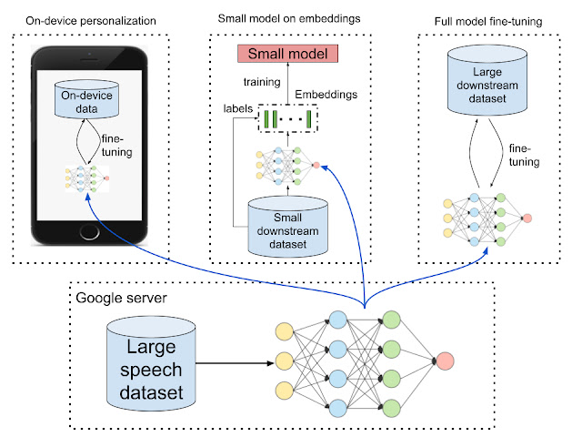
One way to bridge the performance gap between large and small datasets is to train a representation model on a large dataset, then transfer it to a setting with less data. Representations can improve performance in two ways: they can make it possible to train small models by transforming high-dimensional data (like images and audio) to a lower dimension, and the representation model can also be used as pre-training. In addition, if the representation model is small enough to be run or trained on-device, it can improve performance in a privacy-preserving way by giving users the benefits of a personalized model where the raw data never leaves their device. While representation learning is commonly used in the text domain (e.g. BERT and ALBERT) and in the images domain (e.g. Inception layers and SimCLR), such approaches are underutilized in the speech domain.
Bottom:A large speech dataset is used to train a model, which is then rolled out to other environments. Top Left: On-device personalization — personalized, on-device models combine security and privacy. Top Middle: Small model on embeddings — general-use representations transform high-dimensional, few-example datasets to a lower dimension without sacrificing accuracy; smaller models train faster and are regularized. Top Right: Full model fine-tuning — large datasets can use the embedding model as pre-training to improve performance
Unambiguously improving generally-useful representations, for non-semantic speech tasks in particular, is difficult without a standard benchmark to compare "speech representation usefulness." While the T5 framework systematically evaluates text embeddings and the Visual Task Adaptation Benchmark (VTAB) standardizes image embedding evaluation, both leading to progress in representation learning in those respective fields, there has been no such benchmark for non-semantic speech embeddings.

In "Towards Learning a Universal Non-Semantic Representation of Speech", we make three contributions to representation learning for speech-related applications. First, we present a NOn-Semantic Speech (NOSS) benchmark for comparing speech representations, which includes diverse datasets and benchmark tasks, such as speech emotion recognition, language identification, and speaker identification. These datasets are available in the "audio" section of TensorFlow Datasets. Second, we create and open-source TRIpLet Loss network (TRILL), a new model that is small enough to be executed and fine-tuned on-device, while still outperforming other representations. Third, we perform a large-scale study comparing different representations, and open-source the code used to compute the performance on new representations.

A New Benchmark for Speech Embeddings
For a benchmark to usefully guide model development, it must contain tasks that ought to have similar solutions and exclude those that are significantly different. Previous work either dealt with the variety of possible speech-based tasks independently, or lumped semantic and non-semantic tasks together. Our work improves performance on non-semantic speech tasks, in part, by focusing on neural network architectures that perform well specifically on this subset of speech tasks.

The tasks were selected for the NOSS benchmark on the basis of their 1) diversity — they need to cover a range of use-cases; 2) complexity — they should be challenging; and 3) availability, with particular emphasis on those tasks that are open-source. We combined six datasets of different sizes and tasks.
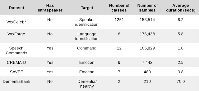
Datasets for downstream benchmark tasks. *VoxCeleb results in our study were computed using a subset of the dataset that was filtered according to internal policy.
We also introduce three additional intra-speaker tasks to test performance in the personalization scenario. In some datasets with k speakers, we can create k different tasks consisting of training and testing on just a single speaker. Overall performance is averaged across speakers. These three additional intra-speaker tasks measure the ability of an embedding to adapt to a particular speaker, as would be necessary for personalized, on-device models, which are becoming more important as computation moves to smart phones and the internet of things.

To help enable researchers to compare speech embeddings, we’ve added the six datasets in our benchmark to TensorFlow Datasets (in the "audio" section) and open sourced the evaluation framework.

TRILL: A New State of the Art in Non-semantic Speech Classification
Learning an embedding from one dataset and applying it to other tasks is not as common in speech as in other modalities. However, transfer learning, the more general technique of using data from one task to help another (not necessarily with embeddings), has some compelling applications, such as personalizing speech recognizers and voice imitation text-to-speech from few samples. There have been many previously proposed representations of speech, but most of these have been trained on a smaller and less diverse data, have been tested primarily on speech recognition, or both.

To create a data-derived representation of speech that was useful across environments and tasks, we started with AudioSet, a large and diverse dataset that includes about 2500 hours of speech. We then trained an embedding model on a simple, self-supervised criteria derived from previous work on metric learning — embeddings from the same audio should be closer in embedding space than embeddings from different audio. Like BERT and the other text embeddings, the self-supervised loss function doesn't require labels and only relies on the structure of the data itself. This form of self-supervision is the most appropriate for non-semantic speech, since non-semantic phenomena are more stable in time than ASR and other sub-second speech characteristics. This simple, self-supervised criteria captures a large number of acoustic properties that are leveraged in downstream tasks.
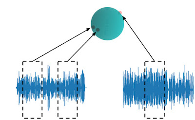
TRILL loss: Embeddings from the same audio are closer in embedding space than embeddings from different audio.
TRILL architecture is based on MobileNet, making it fast enough to run on mobile devices. To achieve high accuracy on this small architecture, we distilled the embedding from a larger ResNet50 model without performance degradation.

Benchmark Results
We compared the performance of TRILL against other deep learning representations that are not focused on speech recognition and were trained on similarly diverse datasets. In addition, we compared TRILL to the popular OpenSMILE feature extractor, which uses pre-deep learning techniques (e.g., a fourier transform coefficients, "pitch tracking" using a time-series of pitch measurements, etc.), and randomly initialized networks, which have been shown to be strong baselines. To aggregate the performance across tasks that have different performance characteristics, we first train a small number of simple models, for a given task and embedding. The best result is chosen. Then, to understand the effect that a particular embedding has across all tasks, we calculate a linear regression on the observed accuracies, with both the model and task as the explanatory variables. The effect a model has on the accuracy is the coefficient associated with the model in the regression. For a given task, when changing from one model to another, the resulting change in accuracy is expected to be the difference in y-values in the figure below.
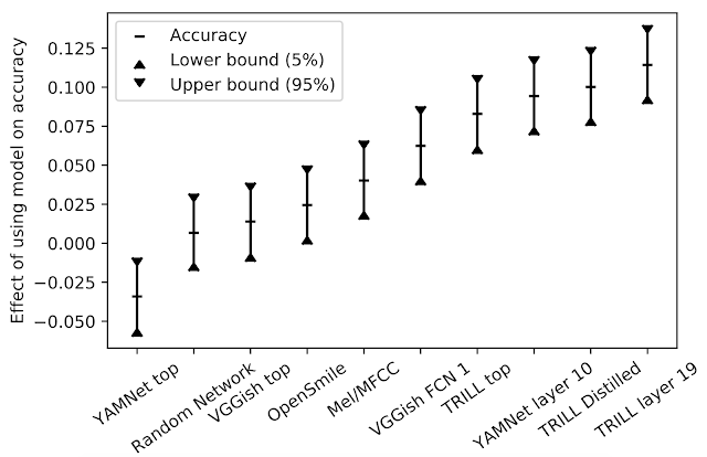
Effect of model on accuracy.
TRILL outperforms the other representations in our study. Factors that contribute to TRILL's success are the diversity of the training dataset, the large context window of the network, and the generality of the TRILL training loss that broadly preserves acoustic characteristics instead of prematurely focusing on certain aspects. Note that representations from intermediate network layers are often more generally useful. The intermediate representations are larger, have finer temporal granularity, and in the case of the classification networks they retain more general information that isn't as specific to the classes on which they were trained.

Another benefit of a generally-useful model is that it can be used to initialize a model on a new task. When the sample size of a new task is small, fine-tuning an existing model may lead to better results than training the model from scratch. We achieved a new state-of-the-art result on three out of six benchmark tasks using this technique, despite doing no dataset-specific hyperparameter tuning.

To compare our new representation, we also tested it on the mask sub-challenge of the Interspeech 2020 Computational Paralinguistics Challenge (ComParE). In this challenge, models must predict whether a speaker is wearing a mask, which would affect their speech. The mask effects are sometimes subtle, and audio clips are only one second long. A linear model on TRILL outperformed the best baseline model, which was a fusion of many models on different kinds of features including traditional spectral and deep-learned features.

Summary
The code to evaluate NOSS is available on GitHub, the datasets are on TensorFlow Datasets, and the TRILL models are available on AI Hub.

The NOn-Semantic Speech benchmark helps researchers create speech embeddings that are useful in a wide range of contexts, including for personalization and small-dataset problems. We provide the TRILL model to the research community as a baseline embedding to surpass.

Acknowledgements
The core team behind this work includes Joel Shor, Aren Jansen, Ronnie Maor, Oran Lang, Omry Tuval, Felix de Chaumont Quitry, Marco Tagliasacchi, Ira Shavitt, Dotan Emanuel, and Yinnon Haviv. We'd also like to thank Avinatan Hassidim and Yossi Matias for technical guidance.
Source: Google AI Blog


Federated Analytics: Collaborative Data Science without Data Collection


Federated learning, introduced in 2017, enables developers to train machine learning (ML) models across many devices without centralized data collection, ensuring that only the user has a copy of their data, and is used to power experiences like suggesting next words and expressions in Gboard for Android and improving the quality of smart replies in Android Messages. Following the success of these applications, there is a growing interest in using federated technologies to answer more basic questions about decentralized data — like computing counts or rates — that often don’t involve ML at all. Analyzing user behavior through these techniques can lead to better products, but it is essential to ensure that the underlying data remains private and secure.

Today we’re introducing federated analytics, the practice of applying data science methods to the analysis of raw data that is stored locally on users’ devices. Like federated learning, it works by running local computations over each device’s data, and only making the aggregated results — and never any data from a particular device — available to product engineers. Unlike federated learning, however, federated analytics aims to support basic data science needs. This post describes the basic methodologies of federated analytics that were developed in the pursuit of federated learning, how we extended those insights into new domains, and how recent advances in federated technologies enable better accuracy and privacy for a growing range of data science needs.

Origin of Federated Analytics
The first exploration into federated analytics was in support of federated learning: how can engineers measure the quality of federated learning models against real-world data when that data is not available in a data center? The answer was to re-use the federated learning infrastructure but without the learning part. In federated learning, the model definition can include not only the loss function that is to be optimized, but also code to compute metrics that indicate the quality of the model’s predictions. We could use this code to directly evaluate model quality on phones’ data.

As an example, Gboard engineers measured the overall quality of next word prediction models against raw typing data held on users’ phones. Participating phones downloaded a candidate model, locally computed a metric of how well the model’s predictions matched the words that were actually typed, and then uploaded the metric without any adjustment to the model’s weights or any change to the Gboard typing experience. By averaging the metrics uploaded by many phones, engineers learned a population-level summary of model performance. The technique also easily extended to estimate basic statistics like dataset sizes.

Federated Analytics for Song Recognition Measurement
Beyond model evaluation, federated analytics is used to support the Now Playing feature on Google’s Pixel phones, a tool that shows you what song is playing in the room around you. Under the hood, Now Playing uses an on-device database of song fingerprints to identify music playing near the phone without the need for a network connection. The architecture is good for privacy and for users — it is fast, works offline, and no raw or processed audio data leaves the phone. Because every phone in a region receives the same database, and only songs in the database can be recognized, it’s important for the database to hold the right songs.

To measure and improve each regional database quality, engineers needed to answer a basic question: which of its songs are most often recognized? Federated analytics provides an answer without revealing which songs are heard by any individual phone. It is enabled for users who agreed to send device related usage and diagnostics information to Google.

When Now Playing recognizes a song, it records the track name into the on-device Now Playing history, where users can see recently recognized songs and add them to a music app’s playlist. Later, when the phone is idle, plugged in, and connected to WiFi, Google’s federated learning and analytics server may invite the phone to join a “round” of federated analytics computation, along with several hundred other phones. Each phone in the round computes the recognition rate for the songs in its Now Playing History, and uses the secure aggregation protocol to encrypt the results. The encrypted rates are sent to the federated analytics server, which does not have the keys to decrypt them individually. But when combined with the encrypted counts from the other phones in the round, the final tally of all song counts (and nothing else) can be decrypted by the server.

The result enables Google engineers to improve the song database (for example, by making sure the database contains truly popular songs), without any phone revealing which songs were heard. In its first improvement iteration, this resulted in a 5% increase in overall song recognition across all Pixel phones globally.

Protecting Federated Analytics with Secure Aggregation
Secure aggregation can enable stronger privacy properties for federated analytics applications. For intuition about the secure aggregation protocol, consider a simpler version of the song recognition measurement problem. Let’s say that Rakshita wants to know how often her friends Emily and Zheng have listened to a particular song. Emily has heard it SEmily times and Zheng SZheng times, but neither is comfortable sharing their counts with Rakshita or each other. Instead, the trio could perform a secure aggregation: Emily and Zheng meet to decide on a random number M, which they keep secret from Rakshita. Emily reveals to Rakshita the sum SEmily + M, while Zheng reveals the difference SZheng - M. Rakshita sees two numbers that are effectively random (they are masked by M), but she can add them together (SEmily + M) + (SZheng - M) = SEmily + SZheng to reveal the total number of times that the song was heard by both Emily and Zheng.

The privacy properties of this approach can be strengthened by summing over more people or by adding small random values to the counts (e.g. in support of differential privacy). For Now Playing, song recognition rates from hundreds of devices are summed together, before the result is revealed to the engineers.
An illustration of the secure aggregation protocol, from the federated learning comic book.
Toward Learning and Analytics with Greater Privacy
The methods of federated analytics are an active area of research and already go beyond analyzing metrics and counts. Sometimes, training ML models with federated learning can be used for obtaining aggregate insights about on-device data, without any of the raw data leaving the devices. For example, Gboard engineers wanted to discover new words commonly typed by users and add them to dictionaries used for spell-checking and typing suggestions, all without being able to see any words that users typed. They did it by training a character-level recurrent neural network on phones, using only the words typed on these phones that were not already in the global dictionary. No typed words ever left the phones, but the resulting model could then be used in the datacenter to generate samples of frequently typed character sequences - the new words!

We are also developing techniques for answering even more ambiguous questions on decentralized datasets like “what patterns in the data are difficult for my model to recognize?” by training federated generative models. And we’re exploring ways to apply user-level differentially private model training to further ensure that these models do not encode information unique to any one user.

Google’s commitment to our privacy principles means pushing the state of the art in safeguarding user data, be it through differential privacy in the data center or advances in privacy during data collection. Google’s earliest system for decentralized data analysis, RAPPOR, was introduced in 2014, and we’ve learned a lot about making effective decisions even with a great deal of noise (often introduced for local differential privacy) since. Federated analytics continues this line of work.

It’s still early days for the federated analytics approach and more progress is needed to answer many common data science questions with good accuracy. The recent Advances and Open Problems in Federated Learning paper offers a comprehensive survey of federated research, while Federated Heavy Hitters Discovery with Differential Privacy introduces a federated analytics method for the discovery of most frequent items in the dataset. Federated analytics enables us to think about data science differently, with decentralized data and privacy-preserving aggregation in a central role. We welcome new contributions and extensions in this emerging field.

Acknowledgments
This post reflects the work of many people, including Blaise Agüera y Arcas, Galen Andrew, Sean Augenstein, Françoise Beaufays, Kallista Bonawitz, Mingqing Chen, Hubert Eichner, Úlfar Erlingsson, Christian Frank, Anna Goralska, Marco Gruteser, Alex Ingerman, Vladimir Ivanov, Peter Kairouz, Chloé Kiddon, Ben Kreuter, Alison Lentz, Wei Li, Xu Liu, Antonio Marcedone, Rajiv Mathews, Brendan McMahan, Tom Ouyang, Sarvar Patel, Swaroop Ramaswamy, Aaron Segal, Karn Seth, Haicheng Sun, Timon Van Overveldt, Sergei Vassilvitskii, Scott Wegner, Yuanbo Zhang, Li Zhang, and Wennan Zhu.

Source: Google AI Blog


Improving Audio Quality in Duo with WaveNetEQ


Online calls have become an everyday part of life for millions of people by helping to streamline their work and connect them to loved ones. To transmit a call across the internet, the data from calls are split into short chunks, called packets. These packets make their way over the network from the sender to the receiver where they are reassembled to make continuous streams of video and audio. However, packets often arrive at the other end in the wrong order or at the wrong time, an issue generally referred to as jitter, and sometimes individual packets can be lost entirely. Issues such as these lead to lower call quality, since the receiver has to try and fill in the gaps, and are a pervasive problem for both audio and video transmission. For example, 99% of Google Duo calls need to deal with packet losses, excessive jitter or network delays. Of those calls, 20% lose more than 3% of the total audio duration due to network issues, and 10% of calls lose more than 8%.
Simplified diagram of network problems leading to packet loss, which needs to be counteracted by the receiver to allow reliable real-time communication.
In order to ensure reliable real-time communication, it is necessary to deal with packets that are missing when the receiver needs them. Specifically, if new audio is not provided continuously, glitches and gaps will be audible, but repeating the same audio over and over is not an ideal solution, as it produces artifacts and reduces the overall quality of the call. The process of dealing with the missing packets is called packet loss concealment (PLC). The receiver’s PLC module is responsible for creating audio (or video) to fill in the gaps created by packet losses, excessive jitter or temporary network glitches, all three of which result in an absence of data.

To address these audio issues, we present WaveNetEQ, a new PLC system now being used in Duo. WaveNetEQ is a generative model, based on DeepMind’s WaveRNN technology, that is trained using a large corpus of speech data to realistically continue short speech segments enabling it to fully synthesize the raw waveform of missing speech. Because Duo calls are end-to-end encrypted, all processing needs to be done on-device. The WaveNetEQ model is fast enough to run on a phone, while still providing state-of-the-art audio quality and more natural sounding PLC than other systems currently in use.

A New PLC System for Duo
Like many other web-based communication systems, Duo is based on the WebRTC open source project. To conceal the effects of packet loss, WebRTC’s NetEQ component uses signal processing methods, which analyze the speech and produce a smooth continuation that works very well for small losses (20ms or less), but does not sound good when the number of missing packets leads to gaps of 60ms or more. In those latter cases the speech becomes robotic and repetitive, a characteristic sound that is unfortunately familiar to many internet voice callers.

To better manage packet loss, we replace the NetEQ PLC component with a modified version of WaveRNN, a recurrent neural network model for speech synthesis consisting of two parts, an autoregressive network and a conditioning network. The autoregressive network is responsible for the continuity of the signal and provides the short-term and mid-term structure for the speech by having each generated sample depend on the network’s previous outputs. The conditioning network influences the autoregressive network to produce audio that is consistent with the more slowly-moving input features.

However, WaveRNN, like its predecessor WaveNet, was created with the text-to-speech (TTS) application in mind. As a TTS model, WaveRNN is supplied with the information of what it is supposed to say and how to say it. The conditioning network directly receives this information as input in form of the phonemes that make up the words and additional prosody features (i.e., all non-text information like intonation or pitch). In a way, the conditioning network can “see into the future” and then steer the autoregressive network towards the right waveforms to match it. In the case of a PLC system and real-time communication, this context is not provided.

For a functional PLC system, one must both extract contextual information from the current speech (i.e., the past), and generate a plausible sound to continue it. Our solution, WaveNetEQ, does both at the same time, using the autoregressive network to provide the audio continuation during a packet loss event, and the conditioning network to model long term features, like voice characteristics. The spectrogram of the past audio signal is used as input for the conditioning network, which extracts limited information about the prosody and textual content. This condensed information is fed to the autoregressive network, which combines it with the audio of the recent past to predict the next sample in the waveform domain.

This differs slightly from the procedure that was followed during training of the WaveNetEQ model, where the autoregressive network receives the actual sample present in the training data as input for the next step, rather than using the last sample it produced. This process, called teacher forcing, assures that the model learns valuable information, even at an early stage of training when its predictions are still of low quality. Once the model is fully trained and put to use in an audio or video call, teacher forcing is only used to "warm up" the model for the first sample, and after that its own output is passed back as input for the next step.
WaveNetEQ architecture. During inference, we "warm up" the autoregressive network by teacher forcing with the most recent audio. Afterwards, the model is supplied with its own output as input for the next step. A MEL spectrogram from a longer audio part is used as input for the conditioning network.
The model is applied to the audio data in Duo's jitter buffer. Once the real audio continues after a packet loss event, we seamlessly merge the synthetic and real audio stream. In order to find the best alignment between the two signals, the model generates slightly more output than is required and then cross-fades from one to the other. This makes the transition smooth and avoids noticeable noise.
Simulation of PLC events on audio over a moving span of 60 ms. The blue line represents the real audio signal, including past and future parts of the PLC event. At each timestep the orange line represents the synthetic audio WaveNetEQ would predict if the audio were to cut out at the vertical grey line.
60 ms Packet Loss
NetEQ
WaveNetEQ
NetEQ
WaveNetEQ

120 ms Packet Loss
NetEQ
WaveNetEQ
NetEQ
WaveNetEQ
Audio clips: Comparison of WebRTC’s default PLC system, NetEQ, with our model, WaveNetEQ. Audio clips were taken from LibriTTS and 10% of the audio was dropped in 60 or 120 ms chunks and then filled in by the PLC systems.
Ensuring Robustness
One important factor during PLC is the ability of the network to adapt to variable input signals, including different speakers or changes in background noise. In order to ensure the robustness of the model across a wide range of users, we trained WaveNetEQ on a speech dataset that contains over 100 speakers in 48 different languages, which allows the model to learn the characteristics of human speech in general, instead of the properties of a specific language. To ensure WaveNetEQ is able to deal with noisy environments, such as answering your phone in the train station or in the cafeteria, we augment the data by mixing it with a wide variety of background noises.

While our model learns how to plausibly continue speech, this is only true on a short scale — it can finish a syllable but does not predict words, per se. Instead, for longer packet losses we gradually fade out until the model only produces silence after 120 milliseconds. To further ensure that the model is not generating false syllables, we evaluated samples from WaveNetEQ and NetEQ using the Google Cloud Speech-to-Text API and found no significant difference in the word error rate, i.e., how many mistakes were made transcribing the spoken text.

We have been experimenting with WaveNetEQ in Duo, where the feature has demonstrated a positive impact on call quality and user experience. WaveNetEQ is already available in all Duo calls on Pixel 4 phones and is now being rolled out to additional models.

Acknowledgements
The core team includes Alessio Bazzica, Niklas Blum, Lennart Kolmodin, Henrik Lundin, Alex Narest, Olga Sharonova from Google and Tom Walters from DeepMind. We would also like to thank Martin Bruse (Google), Norman Casagrande, Ray Smith, Chenjie Gu and Erich Elsen (DeepMind) for their contributions.

Source: Google AI Blog


Real-Time 3D Object Detection on Mobile Devices with MediaPipe


Object detection is an extensively studied computer vision problem, but most of the research has focused on 2D object prediction. While 2D prediction only provides 2D bounding boxes, by extending prediction to 3D, one can capture an object’s size, position and orientation in the world, leading to a variety of applications in robotics, self-driving vehicles, image retrieval, and augmented reality. Although 2D object detection is relatively mature and has been widely used in the industry, 3D object detection from 2D imagery is a challenging problem, due to the lack of data and diversity of appearances and shapes of objects within a category.

Today, we are announcing the release of MediaPipe Objectron, a mobile real-time 3D object detection pipeline for everyday objects. This pipeline detects objects in 2D images, and estimates their poses and sizes through a machine learning (ML) model, trained on a newly created 3D dataset. Implemented in MediaPipe, an open-source cross-platform framework for building pipelines to process perceptual data of different modalities, Objectron computes oriented 3D bounding boxes of objects in real-time on mobile devices.
 
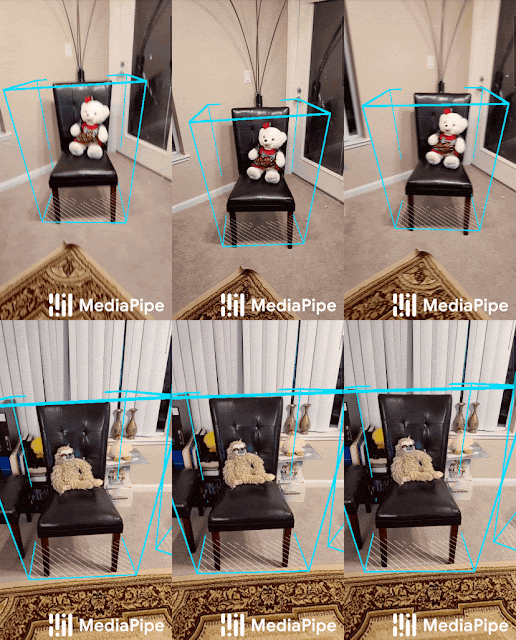
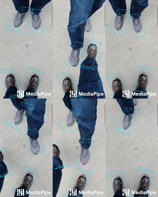
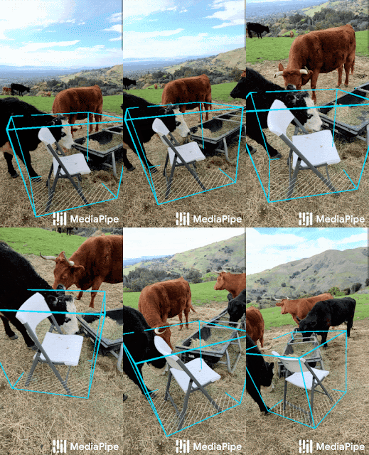
3D Object Detection from a single image. MediaPipe Objectron determines the position, orientation and size of everyday objects in real-time on mobile devices.
Obtaining Real-World 3D Training Data
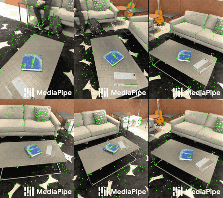
While there are ample amounts of 3D data for street scenes, due to the popularity of research into self-driving cars that rely on 3D capture sensors like LIDAR, datasets with ground truth 3D annotations for more granular everyday objects are extremely limited. To overcome this problem, we developed a novel data pipeline using mobile augmented reality (AR) session data. With the arrival of ARCore and ARKit, hundreds of millions of smartphones now have AR capabilities and the ability to capture additional information during an AR session, including the camera pose, sparse 3D point clouds, estimated lighting, and planar surfaces.

In order to label ground truth data, we built a novel annotation tool for use with AR session data, which allows annotators to quickly label 3D bounding boxes for objects. This tool uses a split-screen view to display 2D video frames on which are overlaid 3D bounding boxes on the left, alongside a view showing 3D point clouds, camera positions and detected planes on the right. Annotators draw 3D bounding boxes in the 3D view, and verify its location by reviewing the projections in 2D video frames. For static objects, we only need to annotate an object in a single frame and propagate its location to all frames using the ground truth camera pose information from the AR session data, which makes the procedure highly efficient.
Real-world data annotation for 3D object detection. Right: 3D bounding boxes are annotated in the 3D world with detected surfaces and point clouds. Left: Projections of annotated 3D bounding boxes are overlaid on top of video frames making it easy to validate the annotation.
AR Synthetic Data Generation
A popular approach is to complement real-world data with synthetic data in order to increase the accuracy of prediction. However, attempts to do so often yield poor, unrealistic data or, in the case of photorealistic rendering, require significant effort and compute. Our novel approach, called AR Synthetic Data Generation, places virtual objects into scenes that have AR session data, which allows us to leverage camera poses, detected planar surfaces, and estimated lighting to generate placements that are physically probable and with lighting that matches the scene. This approach results in high-quality synthetic data with rendered objects that respect the scene geometry and fit seamlessly into real backgrounds. By combining real-world data and AR synthetic data, we are able to increase the accuracy by about 10%.
An example of AR synthetic data generation. The virtual white-brown cereal box is rendered into the real scene, next to the real blue book.
An ML Pipeline for 3D Object Detection
We built a single-stage model to predict the pose and physical size of an object from a single RGB image. The model backbone has an encoder-decoder architecture, built upon MobileNetv2. We employ a multi-task learning approach, jointly predicting an object's shape with detection and regression. The shape task predicts the object's shape signals depending on what ground truth annotation is available, e.g. segmentation. This is optional if there is no shape annotation in training data. For the detection task, we use the annotated bounding boxes and fit a Gaussian to the box, with center at the box centroid, and standard deviations proportional to the box size. The goal for detection is then to predict this distribution with its peak representing the object’s center location. The regression task estimates the 2D projections of the eight bounding box vertices. To obtain the final 3D coordinates for the bounding box, we leverage a well established pose estimation algorithm (EPnP). It can recover the 3D bounding box of an object, without a priori knowledge of the object dimensions. Given the 3D bounding box, we can easily compute pose and size of the object. The diagram below shows our network architecture and post-processing. The model is light enough to run real-time on mobile devices (at 26 FPS on an Adreno 650 mobile GPU).
Network architecture and post-processing for 3D object detection.
Sample results of our network — [left] original 2D image with estimated bounding boxes, [middle] object detection by Gaussian distribution, [right] predicted segmentation mask.
Detection and Tracking in MediaPipe
When the model is applied to every frame captured by the mobile device, it can suffer from jitter due to the ambiguity of the 3D bounding box estimated in each frame. To mitigate this, we adopt the detection+tracking framework recently released in our 2D object detection and tracking solution. This framework mitigates the need to run the network on every frame, allowing the use of heavier and therefore more accurate models, while keeping the pipeline real-time on mobile devices. It also retains object identity across frames and ensures that the prediction is temporally consistent, reducing the jitter.

For further efficiency in our mobile pipeline, we run our model inference only once every few frames. Next, we take the prediction and track it over time using the approach described in our previous blogs for instant motion tracking and Motion Stills. When a new prediction is made, we consolidate the detection result with the tracking result based on the area of overlap.

To encourage researchers and developers to experiment and prototype based on our pipeline, we are releasing our on-device ML pipeline in MediaPipe, including an end-to-end demo mobile application and our trained models for two categories: shoes and chairs. We hope that sharing our solution with the wide research and development community will stimulate new use cases, new applications, and new research efforts. In the future, we plan to scale our model to many more categories, and further improve our on-device performance.
   
Examples of our 3D object detection in the wild.
Acknowledgements
The research described in this post was done by Adel Ahmadyan, Tingbo Hou, Jianing Wei, Matthias Grundmann, Liangkai Zhang, Jiuqiang Tang, Chris McClanahan, Tyler Mullen, Buck Bourdon, Esha Uboweja, Mogan Shieh, Siarhei Kazakou, Ming Guang Yong, Chuo-Ling Chang, and James Bruce. We thank Aliaksandr Shyrokau and the annotation team for their diligence to high quality annotations.

Source: Google AI Blog


The On-Device Machine Learning Behind Recorder


Over the past two decades, Google has made information widely accessible through search — from textual information, photos and videos, to maps and jobs. But much of the world’s information is conveyed through speech. Yet even though many people use audio recording devices to capture important information in conversations, interviews, lectures and more, it can be very difficult to later parse through hours of recordings to identify and extract information of interest. But what if there was the ability to automatically transcribe and tag long recordings in real-time, enabling you to intuitively find the relevant information you need, when you need it?

For this reason, we launched Recorder, a new kind of audio recording app for Pixel phones that leverages recent developments in on-device machine learning (ML) to transcribe conversations, to detect and identify the type of audio recorded (from broad categories like music or speech to particular sounds, such as applause, laughter and whistling), and to index recordings so users can quickly find and extract segments of interest. All of these features run entirely on-device, without the need for an internet connection.
Transcription
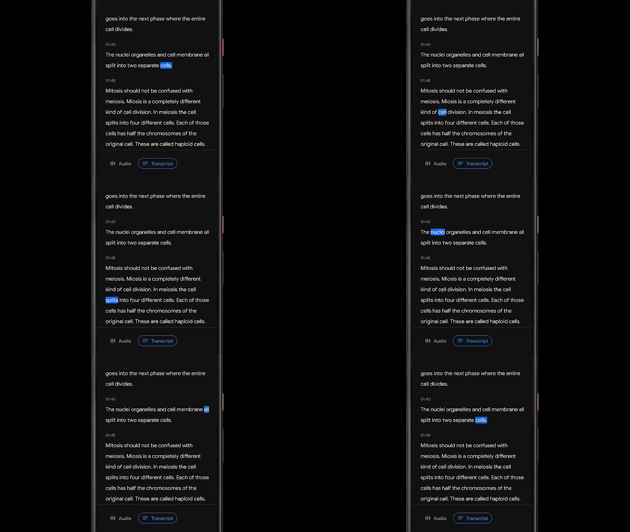
Recorder transcribes speech in real-time using an on-device automatic speech recognition model based on improvements announced earlier this year. Being a key component to many of Recorder’s smart features, we made sure that this model can transcribe long audio recordings (a few hours) reliably, while also indexing conversation by mapping words to timestamps as computed by the speech recognition model. This enables the user to click on a word in the transcription and initiate playback starting from that point in the recording, or to search for a word and jump to the exact point in the recording where it was being said.
Recording Content Visualization via Sound Classification
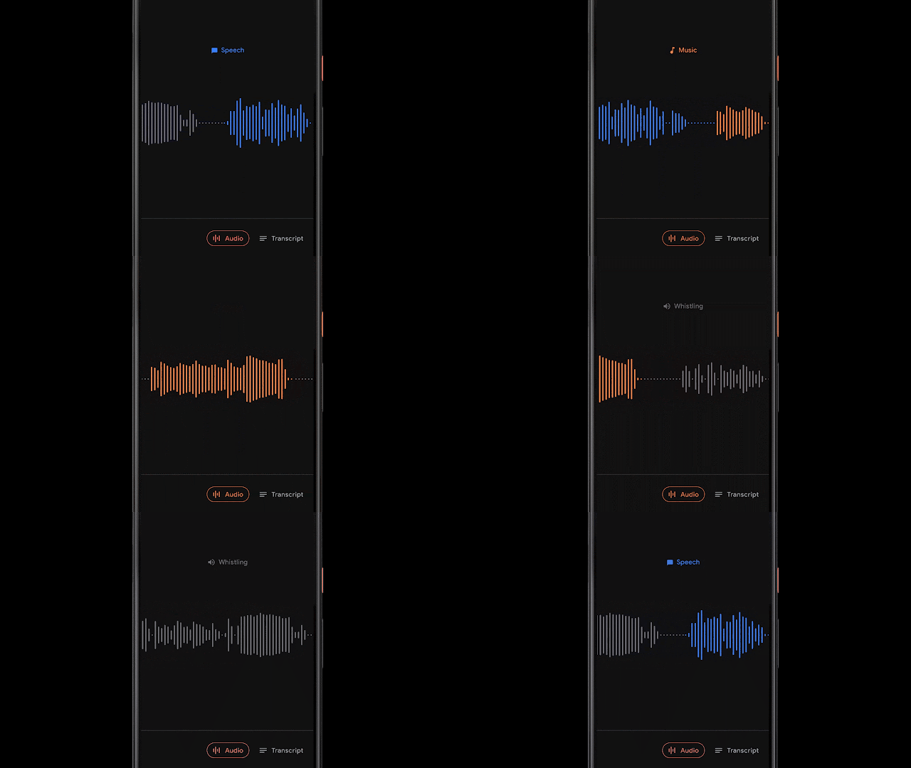
While presenting a transcript for a recording is useful and allows one to search for specific words, sometimes (especially for very long recordings) it’s more useful to visually search for sections of a recording based on specific moments or sounds. To enable this, Recorder additionally represents audio visually as a colored waveform where each color is associated with a different sound category. This is done by combining research into using CNNs to classify audio sounds (e.g., identifying a dog barking or a musical instrument playing) with previously published datasets for audio event detection to classify apparent sound events in individual audio frames.

Of course, in most situations many sounds can appear at the same time. In order to visualize the audio in a very clear way, we decided to color each waveform bar in a single color that represents the most dominant sound in a given time frame (in our case, 50ms bars). The colorized waveform lets users understand what type of content was captured in a specific recording and navigate along an ever-growing audio library more easily. This brings a visual representation of the audio recordings to the users, and also enables them to search over audio events in their recordings.
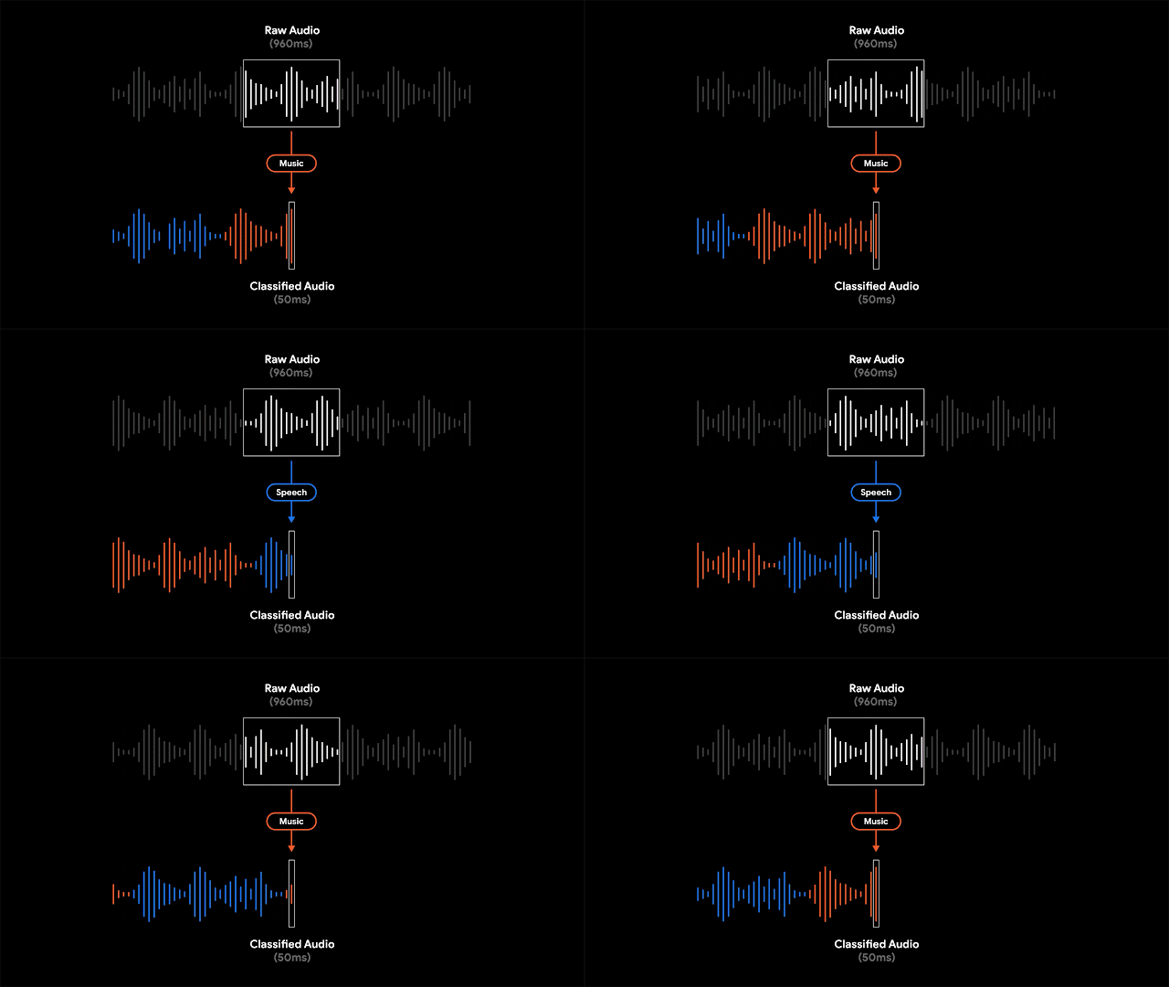
Recorder implements a sliding window capability that processes partially overlapping 960ms audio frames at 50ms intervals and outputs a sigmoid scores vector, representing the probability for each supported audio class within the frame. We apply a linearization process on the sigmoid scores in combination with a thresholding mechanism, in order to maximize the system precision and report the correct sound classification. This process of analyzing the content of the 960ms window with small 50ms offsets makes it possible to pinpoint exact start and end times in a manner that is less prone to mistakes than analyzing consecutive large 960ms window slices on their own.
Since the model analyzes each audio frame independently, it can be prone to quick jittering between audio classes. This is solved with an adaptive-size median filtering technique applied to the most recent model audio class outputs, thus providing a smoothed consecutive output. The process runs continuously in real-time, requiring it to meet very strict power consumption limitations.

Suggesting Tags for Titles
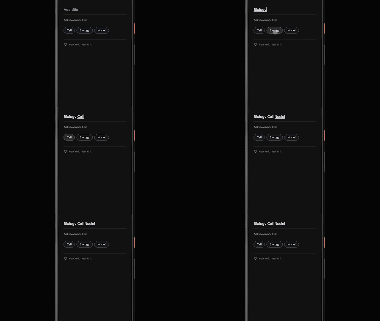
Once a recording is done, Recorder suggests three tags that the app deems to represent the most memorable content, enabling the user to quickly compose a meaningful title.
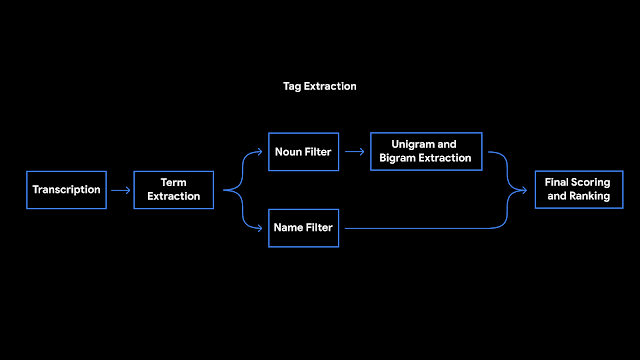
To be able to suggest these tags immediately when the recording ends, Recorder analyzes the content of the recording as it is being transcribed. First, Recorder counts term occurrences as well as their grammatical role in the sentence. The terms identified as entities are capitalized. Then, we utilize an on-device part-of-speech-tagger — a model that labels each word in the sentence according to its grammatical role — to detect common nouns and proper nouns, which appear to be more memorable by users. Recorder utilizes a prior scores table supporting both unigram and bigram terms extraction. To generate the scores, we trained a boosted decision tree with conversational data and utilized textual features like document words frequency and specificity. Last, filtering of stop words and swear words is applied and the top tags are outputted.
Tags extraction pipeline architecture
Conclusion
Recorder galvanized some of our most recent on-device ML research efforts into helpful features, running models on-device to ensure user privacy. The positive feedback loop between machine learning investigations and user needs revealed exciting opportunities to make our software even more useful. We’re excited for future research that will make everyone’s ideas and conversations even more easily accessible and searchable.

Acknowledgments
Special thanks to Dror Ayalon who played a key role in developing and forming the above features and without whom this blog post wouldn’t have been possible. We would also want to thank all our team members and collaborators who worked on this project with us: Amit Pitaru, Kelsie Van Deman, Isaac Blankensmith, Teo Soares, John Watkinson, Matt Hall, Josh Deitel, Benny Schlesinger, Yoni Tsafir, Michelle Tadmor Ramanovich, Danielle Cohen, Sushant Prakash, Renat Aksitov, Ed West, Max Gubin, Tiantian Zhang, Aaron Cohen, Yunhsuan Sung, Chung-Ching Chang, Nathan Dass, Amin Ahmad, Tiago Camolesi, Guilherme Santos‎, Julio da Silva, Dan Ellis, Qiao Liang, Arun Narayanan‎, Rohit Prabhavalkar, Benyah Shaparenko‎, Alex Salcianu, Mike Tsao, Shenaz Zak, Sherry Lin, James Lemieux, Jason Cho, Thomas Hall‎, Brian Chen, Allen Su, Vincent Peng‎, Richard Chou‎, Henry Liu‎, Edward Chen, Yitong Lin, Tracy Wu, Yvonne Yang‎.

Source: Google AI Blog


On-Device, Real-Time Hand Tracking with MediaPipe


The ability to perceive the shape and motion of hands can be a vital component in improving the user experience across a variety of technological domains and platforms. For example, it can form the basis for sign language understanding and hand gesture control, and can also enable the overlay of digital content and information on top of the physical world in augmented reality. While coming naturally to people, robust real-time hand perception is a decidedly challenging computer vision task, as hands often occlude themselves or each other (e.g. finger/palm occlusions and hand shakes) and lack high contrast patterns.

Today we are announcing the release of a new approach to hand perception, which we previewed CVPR 2019 in June, implemented in MediaPipe—an open source cross platform framework for building pipelines to process perceptual data of different modalities, such as video and audio. This approach provides high-fidelity hand and finger tracking by employing machine learning (ML) to infer 21 3D keypoints of a hand from just a single frame. Whereas current state-of-the-art approaches rely primarily on powerful desktop environments for inference, our method achieves real-time performance on a mobile phone, and even scales to multiple hands. We hope that providing this hand perception functionality to the wider research and development community will result in an emergence of creative use cases, stimulating new applications and new research avenues.
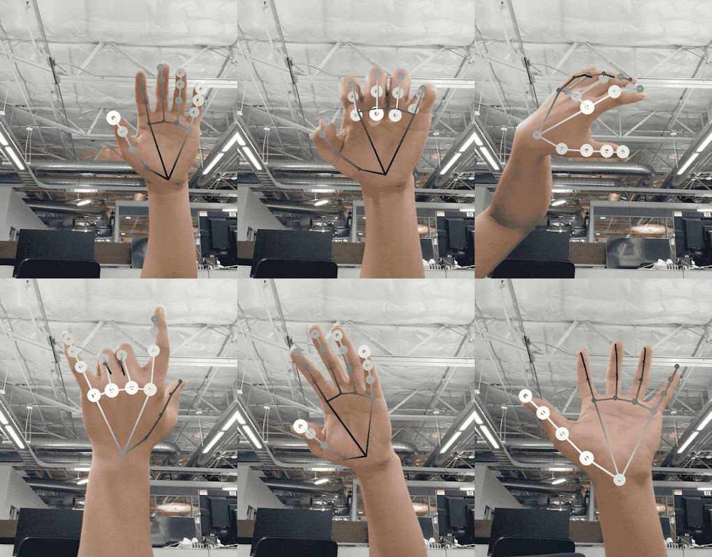
3D hand perception in real-time on a mobile phone via MediaPipe. Our solution uses machine learning to compute 21 3D keypoints of a hand from a video frame. Depth is indicated in grayscale.
An ML Pipeline for Hand Tracking and Gesture Recognition
Our hand tracking solution utilizes an ML pipeline consisting of several models working together:
  • A palm detector model (called BlazePalm) that operates on the full image and returns an oriented hand bounding box.
  • A hand landmark model that operates on the cropped image region defined by the palm detector and returns high fidelity 3D hand keypoints.
  • A gesture recognizer that classifies the previously computed keypoint configuration into a discrete set of gestures.
This architecture is similar to that employed by our recently published face mesh ML pipeline and that others have used for pose estimation. Providing the accurately cropped palm image to the hand landmark model drastically reduces the need for data augmentation (e.g. rotations, translation and scale) and instead allows the network to dedicate most of its capacity towards coordinate prediction accuracy.
Hand perception pipeline overview.
BlazePalm: Realtime Hand/Palm Detection
To detect initial hand locations, we employ a single-shot detector model called BlazePalm, optimized for mobile real-time uses in a manner similar to BlazeFace, which is also available in MediaPipe. Detecting hands is a decidedly complex task: our model has to work across a variety of hand sizes with a large scale span (~20x) relative to the image frame and be able to detect occluded and self-occluded hands. Whereas faces have high contrast patterns, e.g., in the eye and mouth region, the lack of such features in hands makes it comparatively difficult to detect them reliably from their visual features alone. Instead, providing additional context, like arm, body, or person features, aids accurate hand localization.

Our solution addresses the above challenges using different strategies. First, we train a palm detector instead of a hand detector, since estimating bounding boxes of rigid objects like palms and fists is significantly simpler than detecting hands with articulated fingers. In addition, as palms are smaller objects, the non-maximum suppression algorithm works well even for two-hand self-occlusion cases, like handshakes. Moreover, palms can be modelled using square bounding boxes (anchors in ML terminology) ignoring other aspect ratios, and therefore reducing the number of anchors by a factor of 3-5. Second, an encoder-decoder feature extractor is used for bigger scene context awareness even for small objects (similar to the RetinaNet approach). Lastly, we minimize the focal loss during training to support a large amount of anchors resulting from the high scale variance.

With the above techniques, we achieve an average precision of 95.7% in palm detection. Using a regular cross entropy loss and no decoder gives a baseline of just 86.22%.

Hand Landmark Model
After the palm detection over the whole image our subsequent hand landmark model performs precise keypoint localization of 21 3D hand-knuckle coordinates inside the detected hand regions via regression, that is direct coordinate prediction. The model learns a consistent internal hand pose representation and is robust even to partially visible hands and self-occlusions.

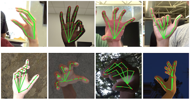
To obtain ground truth data, we have manually annotated ~30K real-world images with 21 3D coordinates, as shown below (we take Z-value from image depth map, if it exists per corresponding coordinate). To better cover the possible hand poses and provide additional supervision on the nature of hand geometry, we also render a high-quality synthetic hand model over various backgrounds and map it to the corresponding 3D coordinates.
Top: Aligned hand crops passed to the tracking network with ground truth annotation. Bottom: Rendered synthetic hand images with ground truth annotation
However, purely synthetic data poorly generalizes to the in-the-wild domain. To overcome this problem, we utilize a mixed training schema. A high-level model training diagram is presented in the following figure.
Mixed training schema for hand tracking network. Cropped real-world photos and rendered synthetic images are used as input to predict 21 3D keypoints.
The table below summarizes regression accuracy depending on the nature of the training data. Using both synthetic and real world data results in a significant performance boost.

Mean regression error
Dataset normalized by palm size
Only real-world 16.1 %
Only rendered synthetic 25.7 %
Mixed real-world + synthetic 13.4 %

Gesture Recognition
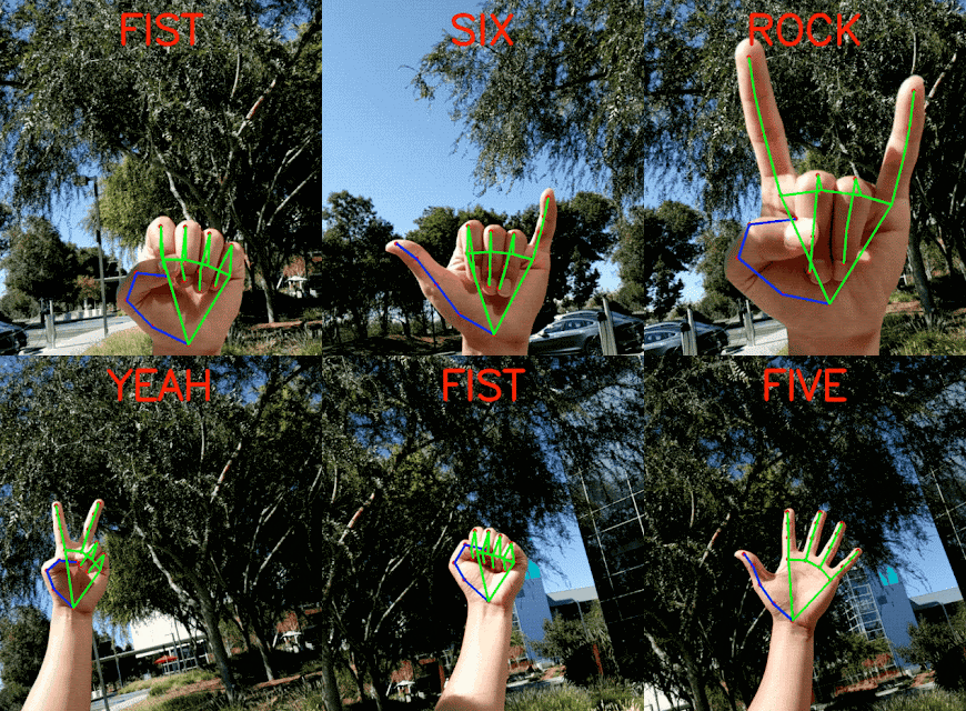
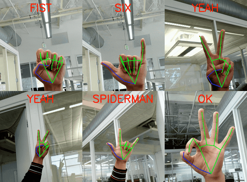
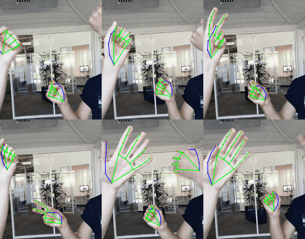
On top of the predicted hand skeleton, we apply a simple algorithm to derive the gestures. First, the state of each finger, e.g. bent or straight, is determined by the accumulated angles of joints. Then we map the set of finger states to a set of pre-defined gestures. This straightforward yet effective technique allows us to estimate basic static gestures with reasonable quality. The existing pipeline supports counting gestures from multiple cultures, e.g. American, European, and Chinese, and various hand signs including “Thumb up”, closed fist, “OK”, “Rock”, and “Spiderman”.

Implementation via MediaPipe
With MediaPipe, this perception pipeline can be built as a directed graph of modular components, called Calculators. Mediapipe comes with an extendable set of Calculators to solve tasks like model inference, media processing algorithms, and data transformations across a wide variety of devices and platforms. Individual calculators like cropping, rendering and neural network computations can be performed exclusively on the GPU. For example, we employ TFLite GPU inference on most modern phones.

Our MediaPipe graph for hand tracking is shown below. The graph consists of two subgraphs—one for hand detection and one for hand keypoints (i.e., landmark) computation. One key optimization MediaPipe provides is that the palm detector is only run as necessary (fairly infrequently), saving significant computation time. We achieve this by inferring the hand location in the subsequent video frames from the computed hand key points in the current frame, eliminating the need to run the palm detector over each frame. For robustness, the hand tracker model outputs an additional scalar capturing the confidence that a hand is present and reasonably aligned in the input crop. Only when the confidence falls below a certain threshold is the hand detection model reapplied to the whole frame.
The hand landmark model’s output (REJECT_HAND_FLAG) controls when the hand detection model is triggered. This behavior is achieved by MediaPipe’s powerful synchronization building blocks, resulting in high performance and optimal throughput of the ML pipeline.
A highly efficient ML solution that runs in real-time and across a variety of different platforms and form factors involves significantly more complexities than what the above simplified description captures. To this end, we are open sourcing the above hand tracking and gesture recognition pipeline in the MediaPipe framework, accompanied with the relevant end-to-end usage scenario and source code, here. This provides researchers and developers with a complete stack for experimentation and prototyping of novel ideas based on our model.

Future Directions
We plan to extend this technology with more robust and stable tracking, enlarge the amount of gestures we can reliably detect, and support dynamic gestures unfolding in time. We believe that publishing this technology can give an impulse to new creative ideas and applications by the members of the research and developer community at large. We are excited to see what you can build with it!
Acknowledgements
Special thanks to all our team members who worked on the tech with us: Andrey Vakunov, Andrei Tkachenka, Yury Kartynnik, Artsiom Ablavatski, Ivan Grishchenko, Kanstantsin Sokal‎, Mogan Shieh, Ming Guang Yong, Anastasia Tkach, Jonathan Taylor, Sean Fanello, Sofien Bouaziz, Juhyun Lee‎, Chris McClanahan, Jiuqiang Tang‎, Esha Uboweja‎, Hadon Nash‎, Camillo Lugaresi, Michael Hays, Chuo-Ling Chang, Matsvei Zhdanovich and Matthias Grundmann.

Source: Google AI Blog


Custom On-Device ML Models with Learn2Compress


Successful deep learning models often require significant amounts of computational resources, memory and power to train and run, which presents an obstacle if you want them to perform well on mobile and IoT devices. On-device machine learning allows you to run inference directly on the devices, with the benefits of data privacy and access everywhere, regardless of connectivity. On-device ML systems, such as MobileNets and ProjectionNets, address the resource bottlenecks on mobile devices by optimizing for model efficiency. But what if you wanted to train your own customized, on-device models for your personal mobile application?

Yesterday at Google I/O, we announced ML Kit to make machine learning accessible for all mobile developers. One of the core ML Kit capabilities that will be available soon is an automatic model compression service powered by “Learn2Compress” technology developed by our research team. Learn2Compress enables custom on-device deep learning models in TensorFlow Lite that run efficiently on mobile devices, without developers having to worry about optimizing for memory and speed. We are pleased to make Learn2Compress for image classification available soon through ML Kit. Learn2Compress will be initially available to a small number of developers, and will be offered more broadly in the coming months. You can sign up here if you are interested in using this feature for building your own models.

How it Works
Learn2Compress generalizes the learning framework introduced in previous works like ProjectionNet and incorporates several state-of-the-art techniques for compressing neural network models. It takes as input a large pre-trained TensorFlow model provided by the user, performs training and optimization and automatically generates ready-to-use on-device models that are smaller in size, more memory-efficient, more power-efficient and faster at inference with minimal loss in accuracy.
Learn2Compress for automatically generating on-device ML models.
To do this, Learn2Compress uses multiple neural network optimization and compression techniques including:
  • Pruning reduces model size by removing weights or operations that are least useful for predictions (e.g.low-scoring weights). This can be very effective especially for on-device models involving sparse inputs or outputs, which can be reduced up to 2x in size while retaining 97% of the original prediction quality.
  • Quantization techniques are particularly effective when applied during training and can improve inference speed by reducing the number of bits used for model weights and activations. For example, using 8-bit fixed point representation instead of floats can speed up the model inference, reduce power and further reduce size by 4x.
  • Joint training and distillation approaches follow a teacher-student learning strategy — we use a larger teacher network (in this case, user-provided TensorFlow model) to train a compact student network (on-device model) with minimal loss in accuracy.
    Joint training and distillation approach to learn compact student models.
    The teacher network can be fixed (as in distillation) or jointly optimized, and even train multiple student models of different sizes simultaneously. So instead of a single model, Learn2Compress generates multiple on-device models in a single shot, at different sizes and inference speeds, and lets the developer pick one best suited for their application needs.
These and other techniques like transfer learning also make the compression process more efficient and scalable to large-scale datasets.

How well does it work?
To demonstrate the effectiveness of Learn2Compress, we used it to build compact on-device models of several state-of-the-art deep networks used in image and natural language tasks such as MobileNets, NASNet, Inception, ProjectionNet, among others. For a given task and dataset, we can generate multiple on-device models at different inference speeds and model sizes.
Accuracy at various sizes for Learn2Compress models and full-sized baseline networks on CIFAR-10 (left) and ImageNet (right) image classification tasks. Student networks used to produce the compressed variants for CIFAR-10 and ImageNet are modeled using NASNet and MobileNet-inspired architectures, respectively.
For image classification, Learn2Compress can generate small and fast models with good prediction accuracy suited for mobile applications. For example, on ImageNet task, Learn2Compress achieves a model 22x smaller than Inception v3 baseline and 4x smaller than MobileNet v1 baseline with just 4.6-7% drop in accuracy. On CIFAR-10, jointly training multiple Learn2Compress models with shared parameters, takes only 10% more time than training a single Learn2Compress large model, but yields 3 compressed models that are upto 94x smaller in size and upto 27x faster with up to 36x lower cost and good prediction quality (90-95% top-1 accuracy).
Computation cost and average prediction latency (on Pixel phone) for baseline and Learn2Compress models on CIFAR-10 image classification task. Learn2Compress-optimized models use NASNet-style network architecture.
We are also excited to see how well this performs on developer use-cases. For example, Fishbrain, a social platform for fishing enthusiasts, used Learn2Compress to compress their existing image classification cloud model (80MB+ in size and 91.8% top-3 accuracy) to a much smaller on-device model, less than 5MB in size, with similar accuracy. In some cases, we observe that it is possible for the compressed models to even slightly outperform the original large model’s accuracy due to better regularization effects.

We will continue to improve Learn2Compress with future advances in ML and deep learning, and extend to more use-cases beyond image classification. We are excited and looking forward to make this available soon through ML Kit’s compression service on the Cloud. We hope this will make it easy for developers to automatically build and optimize their own on-device ML models so that they can focus on building great apps and cool user experiences involving computer vision, natural language and other machine learning applications.

Acknowledgments
I would like to acknowledge our core contributors Gaurav Menghani, Prabhu Kaliamoorthi and Yicheng Fan along with Wei Chai, Kang Lee, Sheng Xu and Pannag Sanketi. Special thanks to Dave Burke, Brahim Elbouchikhi, Hrishikesh Aradhye, Hugues Vincent, and Arun Venkatesan from the Android team; Sachin Kotwani, Wesley Tarle, Pavel Jbanov and from the Firebase team; Andrei Broder, Andrew Tomkins, Robin Dua, Patrick McGregor, Gaurav Nemade, the Google Expander team and TensorFlow team.


Source: Google AI Blog


Introducing the CVPR 2018 On-Device Visual Intelligence Challenge


Over the past year, there have been exciting innovations in the design of deep networks for vision applications on mobile devices, such as the MobileNet model family and integer quantization. Many of these innovations have been driven by performance metrics that focus on meaningful user experiences in real-world mobile applications, requiring inference to be both low-latency and accurate. While the accuracy of a deep network model can be conveniently estimated with well established benchmarks in the computer vision community, latency is surprisingly difficult to measure and no uniform metric has been established. This lack of measurement platforms and uniform metrics have hampered the development of performant mobile applications.

Today, we are happy to announce the On-device Visual Intelligence Challenge (OVIC), part of the Low-Power Image Recognition Challenge Workshop at the 2018 Computer Vision and Pattern Recognition conference (CVPR2018). A collaboration with Purdue University, the University of North Carolina and IEEE, OVIC is a public competition for real-time image classification that uses state-of-the-art Google technology to significantly lower the barrier to entry for mobile development. OVIC provides two key features to catalyze innovation: a unified latency metric and an evaluation platform.

A Unified Metric
OVIC focuses on the establishment of a unified metric aligned directly with accurate and performant operation on mobile devices. The metric is defined as the number of correct classifications within a specified per-image average time limit of 33ms. This latency limit allows every frame in a live 30 frames-per-second video to be processed, thus providing a seamless user experience1. Prior to OVIC, it was tricky to enforce such a limit due to the difficulty in accurately and uniformly measuring latency as would be experienced in real-world applications on real-world devices. Without a repeatable mobile development platform, researchers have relied primarily on approximate metrics for latency that are convenient to compute, such as the number of multiply-accumulate operations (MACs). The intuition is that multiply-accumulate constitutes the most time-consuming operation in a deep neural network, so their count should be indicative of the overall latency. However, these metrics are often poor predictors of on-device latency due to many aspects of the models that can impact the average latency of each MAC in typical implementations.
Even though the number of multiply-accumulate operations (# MACs) is the most commonly used metric to approximate on-device latency, it is a poor predictor of latency. Using data from various quantized and floating point MobileNet V1 and V2 based models, this graph plots on-device latency on a common reference device versus the number of MACs. It is clear that models with similar latency can have very different MACs, and vice versa.
The graph above shows that while the number of MACs is correlated with the inference latency, there is significant variation in the mapping. Thus number of MACs is a poor proxy for latency, and since latency directly affects users’ experiences, we believe it is paramount to optimize latency directly rather than focusing on limiting the number of MACs as a proxy.

An Evaluation Platform
As mentioned above, a primary issue with latency is that it has previously been challenging to measure reliably and repeatably, due to variations in implementation, running environment and hardware architectures. Recent successes in mobile development overcome these challenges with the help of a convenient mobile development platform, including optimized kernels for mobile CPUs, light-weight portable model formats, increasingly capable mobile devices, and more. However, these various platforms have traditionally required resources and development capabilities that are only available to larger universities and industry.

With that in mind, we are releasing OVIC’s evaluation platform that includes a number of components designed to make mobile development and evaluations that can be replicated and compared accessible to the broader research community:
  • TOCO compiler for optimizing TensorFlow models for efficient inference
  • TensorFlow Lite inference engine for mobile deployment
  • A benchmarking SDK that can be run locally on any Android phone
  • Sample models to showcase successful mobile architectures that run inference in floating-point and quantized modes
  • Google’s benchmarking tool for reliable latency measurements on specific Pixel phones (available to registered contestants).
Using these tools available in OVIC, a participant can conveniently incorporate measurement of on-device latency into their design loop without having to worry about optimizing kernels, purchasing latency/power measurement devices, or designing the framework to drive them. The only requirement for entry is experiences with training computer vision models in TensorFlow, which can be found in this tutorial.

With OVIC, we encourage the entire research community to improve the classification performance of low-latency high-accuracy models towards new frontiers, as shown in the following graphic.
Sampling of current MobileNet mobile models illustrating the tradeoff between increased accuracy and reduced latency.
We cordially invite you to participate here before the deadline on June 15th, and help us discover new mobile vision architectures that will propel development into the future.

Acknowledgements
We would like to acknowledge our core contributors Achille Brighton, Alec Go, Andrew Howard, Hartwig Adam, Mark Sandler and Xiao Zhang. We would also like to acknowledge our external collaborators Alex Berg and Yung-Hsiang Lu. We give special thanks to Andre Hentz, Andrew Selle, Benoit Jacob, Brad Krueger, Dmitry Kalenichenko, Megan Cummins, Pete Warden, Rajat Monga, Shiyu Hu and Yicheng Fan.


1 Alternatively the same metric could encourage even lower power operation by only processing a subset of the images in the input stream.


Source: Google AI Blog