Category Archives: Research Blog

The latest news on Google Research

High-Definition Segmentation in Google Meet

In recent years video conferencing has played an increasingly important role in both work and personal communication for many users. Over the past two years, we have enhanced this experience in Google Meet by introducing privacy-preserving machine learning (ML) powered background features, also known as “virtual green screen”, which allows users to blur their backgrounds or replace them with other images. What is unique about this solution is that it runs directly in the browser without the need to install additional software.

So far, these ML-powered features have relied on CPU inference made possible by leveraging neural network sparsity, a common solution that works across devices, from entry level computers to high-end workstations. This enables our features to reach the widest audience. However, mid-tier and high-end devices often have powerful GPUs that remain untapped for ML inference, and existing functionality allows web browsers to access GPUs via shaders (WebGL).

With the latest update to Google Meet, we are now harnessing the power of GPUs to significantly improve the fidelity and performance of these background effects. As we detail in “Efficient Heterogeneous Video Segmentation at the Edge”, these advances are powered by two major components: 1) a novel real-time video segmentation model and 2) a new, highly efficient approach for in-browser ML acceleration using WebGL. We leverage this capability to develop fast ML inference via fragment shaders. This combination results in substantial gains in accuracy and latency, leading to crisper foreground boundaries.

CPU segmentation vs. HD segmentation in Meet.

Moving Towards Higher Quality Video Segmentation Models
To predict finer details, our new segmentation model now operates on high definition (HD) input images, rather than lower-resolution images, effectively doubling the resolution over the previous model. To accommodate this, the model must be of higher capacity to extract features with sufficient detail. Roughly speaking, doubling the input resolution quadruples the computation cost during inference.

Inference of high-resolution models using the CPU is not feasible for many devices. The CPU may have a few high-performance cores that enable it to execute arbitrary complex code efficiently, but it is limited in its ability for the parallel computation required for HD segmentation. In contrast, GPUs have many, relatively low-performance cores coupled with a wide memory interface, making them uniquely suitable for high-resolution convolutional models. Therefore, for mid-tier and high-end devices, we adopt a significantly faster pure GPU pipeline, which is integrated using WebGL.

This change inspired us to revisit some of the prior design decisions for the model architecture.

  • Backbone: We compared several widely-used backbones for on-device networks and found EfficientNet-Lite to be a better fit for the GPU because it removes the squeeze-and-excitation block, a component that is inefficient on WebGL (more below).
  • Decoder: We switched to a multi-layer perceptron (MLP) decoder consisting of 1x1 convolutions instead of using simple bilinear upsampling or the more expensive squeeze-and-excitation blocks. MLP has been successfully adopted in other segmentation architectures, like DeepLab and PointRend, and is efficient to compute on both CPU and GPU.
  • Model size: With our new WebGL inference and the GPU-friendly model architecture, we were able to afford a larger model without sacrificing the real-time frame rate necessary for smooth video segmentation. We explored the width and the depth parameters using a neural architecture search.
HD segmentation model architecture.

In aggregate, these changes substantially improve the mean Intersection over Union (IoU) metric by 3%, resulting in less uncertainty and crisper boundaries around hair and fingers.

We have also released the accompanying model card for this segmentation model, which details our fairness evaluations. Our analysis shows that the model is consistent in its performance across the various regions, skin-tones, and genders, with only small deviations in IoU metrics.

Model     Resolution     Inference     IoU     Latency (ms)
CPU segmenter     256×144     Wasm SIMD     94.0%     8.7
GPU segmenter     512×288     WebGL     96.9%     4.3
Comparison of the previous segmentation model vs. the new HD segmentation model on a Macbook Pro (2018).

Accelerating Web ML with WebGL
One common challenge for web-based inference is that web technologies can incur a performance penalty when compared to apps running natively on-device. For GPUs, this penalty is substantial, only achieving around 25% of native OpenGL performance. This is because WebGL, the current GPU standard for Web-based inference, was primarily designed for image rendering, not arbitrary ML workloads. In particular, WebGL does not include compute shaders, which allow for general purpose computation and enable ML workloads in mobile and native apps.

To overcome this challenge, we accelerated low-level neural network kernels with fragment shaders that typically compute the output properties of a pixel like color and depth, and then applied novel optimizations inspired by the graphics community. As ML workloads on GPUs are often bound by memory bandwidth rather than compute, we focused on rendering techniques that would improve the memory access, such as Multiple Render Targets (MRT).

MRT is a feature in modern GPUs that allows rendering images to multiple output textures (OpenGL objects that represent images) at once. While MRT was originally designed to support advanced graphics rendering such as deferred shading, we found that we could leverage this feature to drastically reduce the memory bandwidth usage of our fragment shader implementations for critical operations, like convolutions and fully connected layers. We do so by treating intermediate tensors as multiple OpenGL textures.

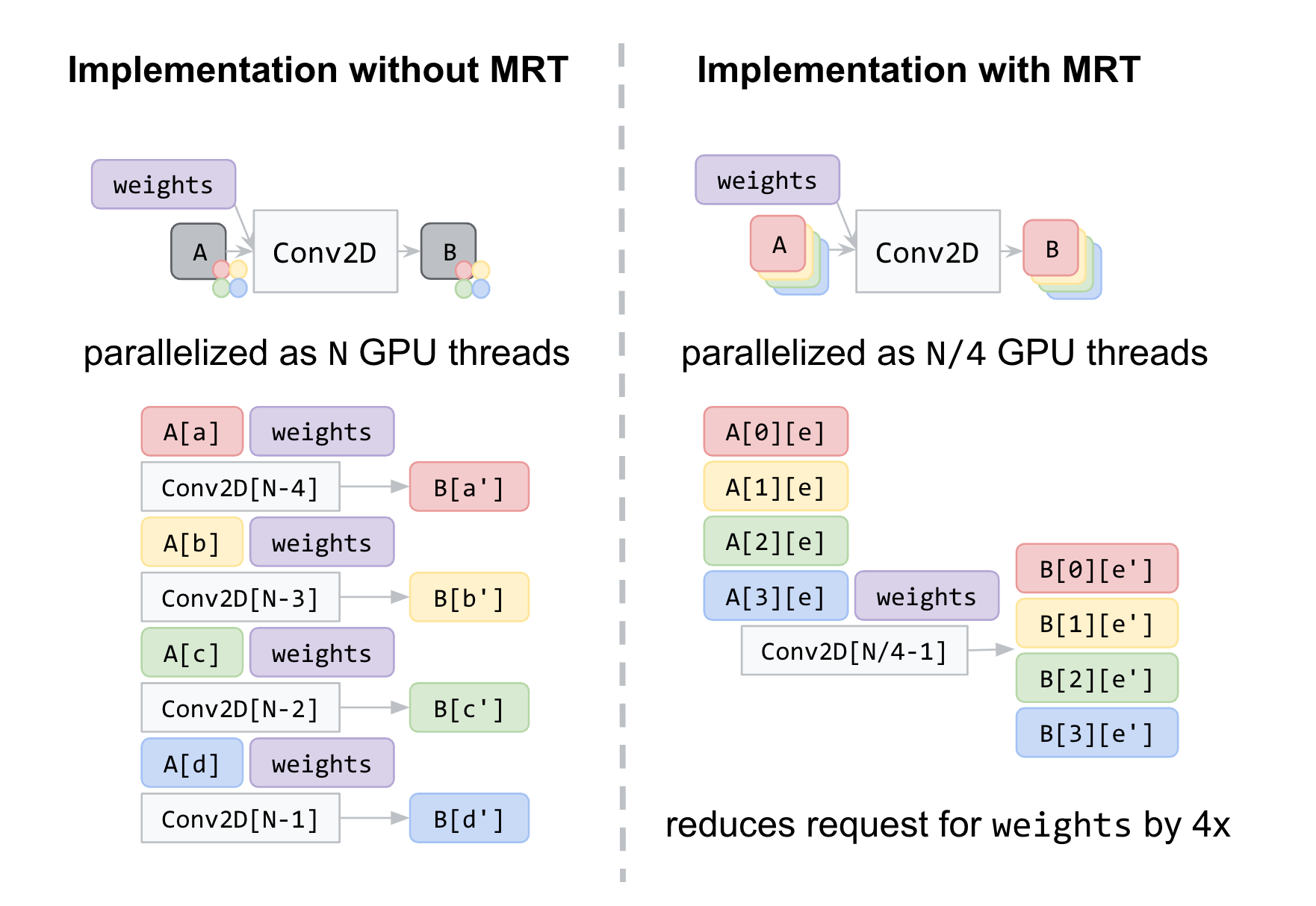
In the figure below, we show an example of intermediate tensors having four underlying GL textures each. With MRT, the number of GPU threads, and thus effectively the number of memory requests for weights, is reduced by a factor of four and saves memory bandwidth usage. Although this introduces considerable complexities in the code, it helps us reach over 90% of native OpenGL performance, closing the gap with native applications.

Left: A classic implementation of Conv2D with 1-to-1 correspondence of tensor and an OpenGL texture. Red, yellow, green, and blue boxes denote different locations in a single texture each for intermediate tensor A and B. Right: Our implementation of Conv2D with MRT where intermediate tensors A and B are realized with a set of 4 GL textures each, depicted as red, yellow, green, and blue boxes. Note that this reduces the request count for weights by 4x.

Conclusion
We have made rapid strides in improving the quality of real-time segmentation models by leveraging the GPU on mid-tier and high-end devices for use with Google Meet. We look forward to the possibilities that will be enabled by upcoming technologies like WebGPU, which bring compute shaders to the web. Beyond GPU inference, we're also working on improving the segmentation quality for lower powered devices with quantized inference via XNNPACK WebAssembly.

Acknowledgements
Special thanks to those on the Meet team and others who worked on this project, in particular Sebastian Jansson, Sami Kalliomäki, Rikard Lundmark, Stephan Reiter, Fabian Bergmark, Ben Wagner, Stefan Holmer, Dan Gunnarsson, Stéphane Hulaud, and to all our team members who made this possible: Siargey Pisarchyk, Raman Sarokin, Artsiom Ablavatski, Jamie Lin, Tyler Mullen, Gregory Karpiak, Andrei Kulik, Karthik Raveendran, Trent Tolley, and Matthias Grundmann.
Source: Google AI Blog


Using ML to Boost Engagement with a Maternal and Child Health Program in India

The widespread availability of mobile phones has enabled non-profits to deliver critical health information to their beneficiaries in a timely manner. While advanced applications on smartphones allow for richer multimedia content and two-way communication between beneficiaries and health coaches, simpler text and voice messaging services can be effective in disseminating information to large communities, particularly those that are underserved with limited access to information and smartphones. ARMMAN1, one non-profit doing just this, is based in India with the mission of improving maternal and child health outcomes in underserved communities.

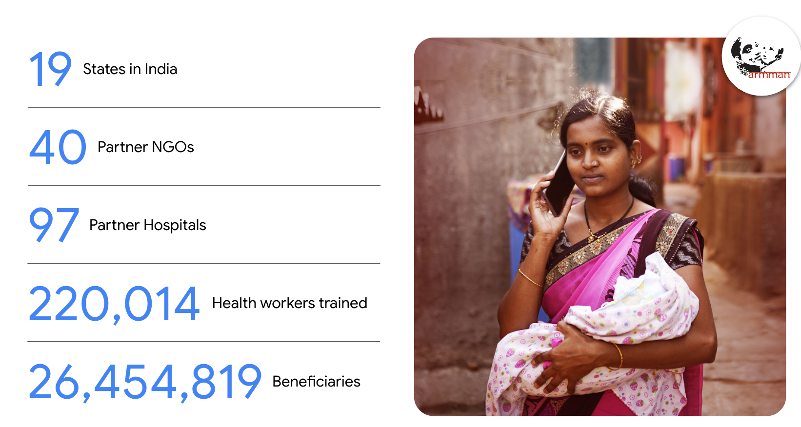
Overview of ARMMAN

One of the programs run by them is mMitra, which employs automated voice messaging to deliver timely preventive care information to expecting and new mothers during pregnancy and until one year after birth. These messages are tailored according to the gestational age of the beneficiary. Regular listenership to these messages has been shown to have a high correlation with improved behavioral and health outcomes, such as a 17% increase in infants with tripled birth weight at end of year and a 36% increase in women knowing the importance of taking iron tablets.

However, a key challenge ARMMAN faced was that about 40% of women gradually stopped engaging with the program. While it’s possible to mitigate this with live service calls to women to explain the advantage of listening to the messages, it is infeasible to call all the low listeners in the program because of limited support staff — this highlights the importance of effectively prioritizing who receives such service calls.

In “Field Study in Deploying Restless Multi-Armed Bandits: Assisting Non-Profits in Improving Maternal and Child Health”, published in AAAI 2022, we describe an ML-based solution that uses historical data from the NGO to predict which beneficiaries will benefit most from service calls. We address the challenges that come with a large-scale real world deployment of such a system and show the usefulness of deploying this model in a real study involving over 23,000 participants. The model showed an increase in listenership of 30% compared to the current standard of care group.

Background
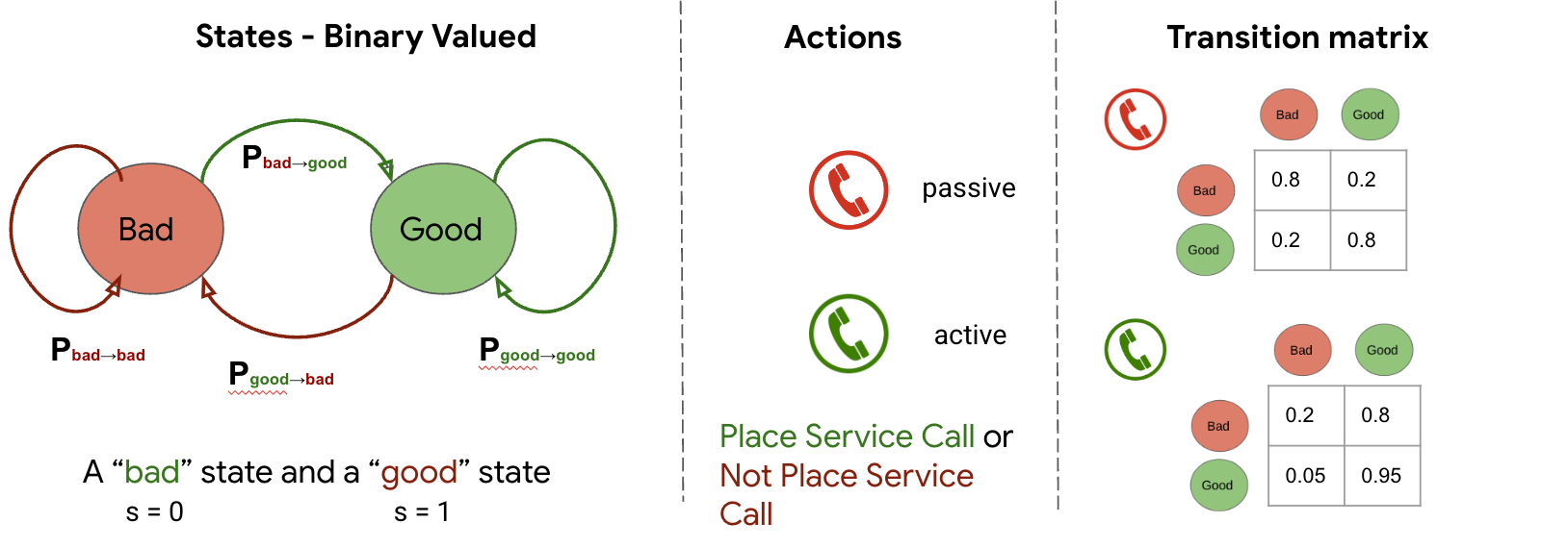
We model this resource optimization problem using restless multi-armed bandits (RMABs), which have been well studied for application to such problems in a myriad of domains, including healthcare. An RMAB consists of n arms where each arm (representing a beneficiary) is associated with a two-state Markov decision process (MDP). Each MDP is modeled as a two-state (good or bad state, where the good state corresponds to high listenership in the previous week), two-action (corresponding to whether the beneficiary was chosen to receive a service call or not) problem. Further, each MDP has an associated reward function (i.e., the reward accumulated at a given state and action) and a transition function indicating the probability of moving from one state to the next under a given action, under the Markov condition that the next state depends only on the previous state and the action taken on that arm in that time step. The term restless indicates that all arms can change state irrespective of the action.

State of a beneficiary may transition from good (high engagement) to bad (low engagement) with example passive and active transition probabilities shown in the transition matrix.

Model Development
Finally, the RMAB problem is modeled such that at any time step, given n total arms, which k arms should be acted on (i.e., chosen to receive a service call), to maximize reward (engagement with the program).

The probability of transitioning from one state to another with (active probability) or without (passive probability) receiving a service call are therefore the underlying model parameters that are critical to solving the above optimization. To estimate these parameters, we use the demographic data of the beneficiaries collected at time of enrolment by the NGO, such as age, income, education, number of children, etc., as well as past listenership data, all in-line with the NGO’s data privacy standards (more below).

However, the limited volume of service calls limits the data corresponding to receiving a service call. To mitigate this, we use clustering techniques to learn from the collective observations of beneficiaries within a cluster and enable overcoming the challenge of limited samples per individual beneficiary.

In particular, we perform clustering on listenership behaviors, and then compute a mapping from the demographic features to each cluster.

Clustering on past listenership data reveals clusters with beneficiaries that behave similarly. We then infer a mapping from demographic features to clusters.

This mapping is useful because when a new beneficiary is enrolled, we only have access to their demographic information and have no knowledge of their listenership patterns, since they haven’t had a chance to listen yet. Using the mapping, we can infer transition probabilities for any new beneficiary that enrolls into the system.

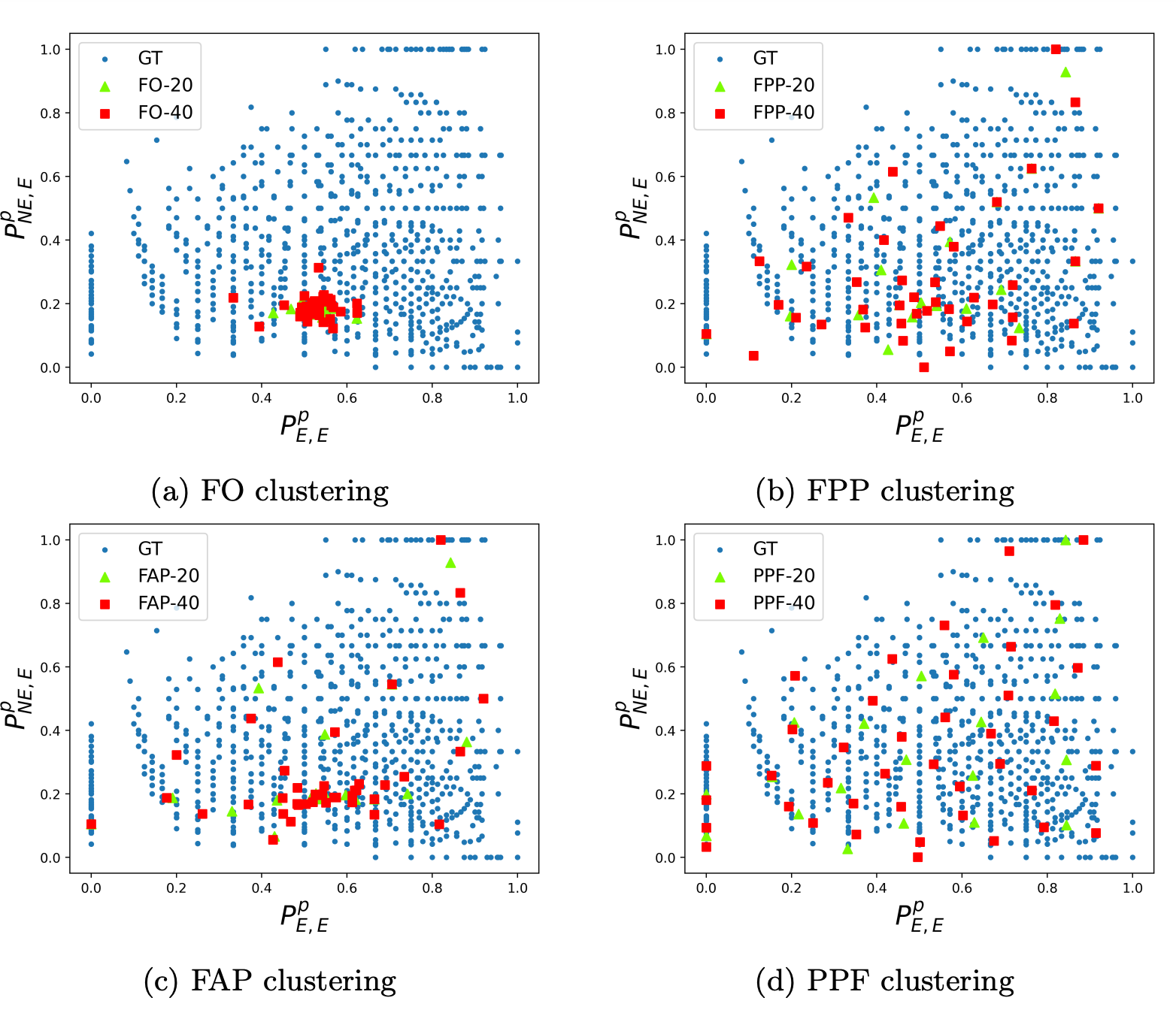
We used several qualitative and quantitative metrics to infer the optimal set of of clusters and explored different combinations of training data (demographic features only, features plus passive probabilities, features plus all probabilities, passive probabilities only) to achieve the most meaningful clusters, that are representative of the underlying data distribution and have a low variance in individual cluster sizes.

Comparison of passive transition probabilities obtained from different clustering methods with number of clusters s = 20 (red dots) and 40 (green dots), using ground truth passive transition probabilities (blue dots). Clustering based on features+passive probabilities (PPF) captures more distinct beneficiary behaviors across the probability space.

Clustering has the added advantage of reducing computational cost for resource-limited NGOs, as the optimization needs to be solved at a cluster level rather than an individual level. Finally, solving RMAB’s is known to be P-space hard, so we choose to solve the optimization using the popular Whittle index approach, which ultimately provides a ranking of beneficiaries based on their likely benefit of receiving a service call.

Results
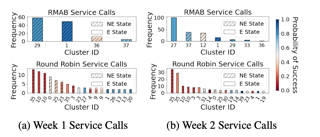
We evaluated the model in a real world study consisting of approximately 23,000 beneficiaries who were divided into three groups: the current standard of care (CSOC) group, the "round robin" (RR) group, and the RMAB group. The beneficiaries in the CSOC group follow the original standard of care, where there are no NGO initiated service calls. The RR group represents the scenario where the NGO often conducts service calls using some systematic set order — the idea here is to have an easily executable policy that services enough of a cross-section of beneficiaries and can be scaled up or down per week based on available resources (this is the approach used by the NGO in this particular case, but the approach may vary for different NGOs). The RMAB group receives service calls as predicted by the RMAB model. All the beneficiaries across the three groups continue to receive the automated voice messages independent of the service calls.

Distributions of clusters picked for service calls by RMAB and RR in week 1 (left) and 2 (right) are significantly different. RMAB is very strategic in picking only a few clusters with a promising probability of success (blue is high and red is low), RR displays no such strategic selection.

At the end of seven weeks, RMAB-based service calls resulted in the highest (and statistically significant) reduction in cumulative engagement drops (32%) compared to the CSOC group.

The plot shows cumulative engagement drops prevented compared to the control group.
   RMAB vs CSOC       RR vs CSOC       RMAB vs RR   
% reduction in cumulative engagement drops    32.0% 5.2% 28.3%
p-value 0.044 0.740 0.098

Ethical Considerations
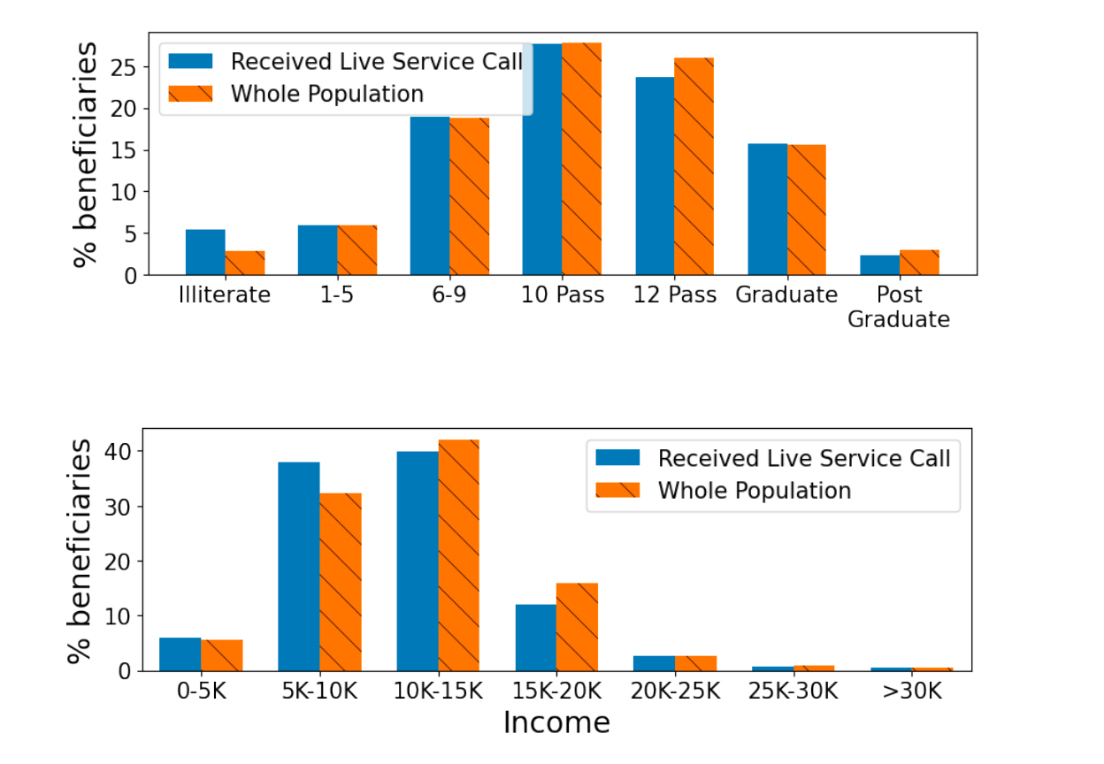
An ethics board at the NGO reviewed the study. We took significant measures to ensure participant consent is understood and recorded in a language of the community's choice at each stage of the program. Data stewardship resides in the hands of the NGO, and only the NGO is allowed to share data. The code will soon be available publicly. The pipeline only uses anonymized data and no personally identifiable information (PII) is made available to the models. Sensitive data, such as caste, religion, etc., are not collected by ARMMAN for mMitra. Therefore, in pursuit of ensuring fairness of the model, we worked with public health and field experts to ensure other indicators of socioeconomic status were measured and adequately evaluated as shown below.

Distribution of highest education received (top) and monthly family income in Indian Rupees (bottom) across a cohort that received service calls compared to the whole population.

The proportion of beneficiaries that received a live service call within each income bracket reasonably matches the proportion in the overall population. However, differences are observed in lower income categories, where the RMAB model favors beneficiaries with lower income and beneficiaries with no formal education. Lastly, domain experts at ARMMAN have been deeply involved in the development and testing of this system and have provided continuous input and oversight in data interpretation, data consumption, and model design.

Conclusions
After thorough testing, the NGO has currently deployed this system for scheduling of service calls on a weekly basis. We are hopeful that this will pave the way for more deployments of ML algorithms for social impact in partnerships with non-profits in service of populations that have so far benefited less from ML. This work was also featured in Google for India 2021.

Acknowledgements
This work is part of our AI for Social Good efforts and was led by Google Research, India. Thanks to all our collaborators at ARMMAN, Google Research India, Google.org, and University Relations: Aparna Hegde, Neha Madhiwalla, Suresh Chaudhary, Aditya Mate, Lovish Madaan, Shresth Verma, Gargi Singh, Divy Thakkar.


1ARMMAN runs multiple programs to provide preventive care information to women through pregnancy and infancy enabling them to seek care, as well as programs to train and support health workers for timely detection and management of high-risk conditions. 

Source: Google AI Blog


UVQ: Measuring YouTube’s Perceptual Video Quality

Online video sharing platforms, like YouTube, need to understand perceptual video quality (i.e., a user's subjective perception of video quality) in order to better optimize and improve user experience. Video quality assessment (VQA) attempts to build a bridge between video signals and perceptual quality by using objective mathematical models to approximate the subjective opinions of users. Traditional video quality metrics, like peak signal-to-noise ratio (PSNR) and Video Multi-Method Assessment Fusion (VMAF), are reference-based and focus on the relative difference between the target and reference videos. Such metrics, which work best on professionally generated content (e.g., movies), assume the reference video is of pristine quality and that one can induce the target video's absolute quality from the relative difference.

However, the majority of the videos that are uploaded on YouTube are user-generated content (UGC), which bring new challenges due to their remarkably high variability in video content and original quality. Most UGC uploads are non-pristine and the same amount of relative difference could imply very different perceptual quality impacts. For example, people tend to be less sensitive to the distortions of poor quality uploads than of high quality uploads. Thus, reference-based quality scores become inaccurate and inconsistent when used for UGC cases. Additionally, despite the high volume of UGC, there are currently limited UGC video quality assessment (UGC-VQA) datasets with quality labels. Existing UGC-VQA datasets are either small in size (e.g., LIVE-Qualcomm has 208 samples captured from 54 unique scenes), compared with datasets with millions of samples for classification and recognition (e.g., ImageNet and YouTube-8M), or don’t have enough content variability (sampling without considering content information, like LIVE-VQC and KoNViD-1k).

In "Rich Features for Perceptual Quality Assessment of UGC Videos", published at CVPR 2021, we describe how we attempt to solve the UGC quality assessment problem by building a Universal Video Quality (UVQ) model that resembles a subjective quality assessment. The UVQ model uses subnetworks to analyze UGC quality from high-level semantic information to low-level pixel distortions, and provides a reliable quality score with rationale (leveraging comprehensive and interpretable quality labels). Moreover, to advance UGC-VQA and compression research, we enhance the open-sourced YouTube-UGC dataset, which contains 1.5K representative UGC samples from millions of UGC videos (distributed under the Creative Commons license) on YouTube. The updated dataset contains ground-truth labels for both original videos and corresponding transcoded versions, enabling us to better understand the relationship between video content and its perceptual quality.

Subjective Video Quality Assessment
To understand perceptual video quality, we leverage an internal crowd-sourcing platform to collect mean opinion scores (MOS) with a scale of 1–5, where 1 is the lowest quality and 5 is the highest quality, for no-reference use cases. We collect ground-truth labels from the YouTube-UGC dataset and categorize UGC factors that affect quality perception into three high-level categories: (1) content, (2) distortions, and (3) compression. For example, a video with no meaningful content won't receive a high quality MOS. Also, distortions introduced during the video production phase and video compression artifacts introduced by third-party platforms, e.g., transcoding or transmission, will degrade the overall quality.

MOS= 2.052 MOS= 4.457
Left: A video with no meaningful content won't receive a high quality MOS. Right: A video displaying intense sports shows a higher MOS.
MOS= 1.242 MOS= 4.522
Left: A blurry gaming video gets a very low quality MOS. Right: A video with professional rendering (high contrast and sharp edges, usually introduced in the video production phase) shows a high quality MOS.
MOS= 2.372 MOS= 4.646
Left: A heavily compressed video receives a low quality MOS. Right: a video without compression artifacts shows a high quality MOS.

We demonstrate that the left gaming video in the second row of the figure above has the lowest MOS (1.2), even lower than the video with no meaningful content. A possible explanation is that viewers may have higher video quality expectations for videos that have a clear narrative structure, like gaming videos, and the blur artifacts significantly reduce the perceptual quality of the video.

UVQ Model Framework
A common method for evaluating video quality is to design sophisticated features, and then map these features to a MOS. However, designing useful handcrafted features is difficult and time-consuming, even for domain experts. Also, the most useful existing handcrafted features were summarized from limited samples, which may not perform well on broader UGC cases. In contrast, machine learning is becoming more prominent in UGC-VQA because it can automatically learn features from large-scale samples.

A straightforward approach is to train a model from scratch on existing UGC quality datasets. However, this may not be feasible as there are limited quality UGC datasets. To overcome this limitation, we apply a self-supervised learning step to the UVQ model during training. This self-supervised step enables us to learn comprehensive quality-related features, without ground-truth MOS, from millions of raw videos.

Following the quality-related categories summarized from the subjective VQA, we develop the UVQ model with four novel subnetworks. The first three subnetworks, which we call ContentNet, DistortionNet and CompressionNet, are used to extract quality features (i.e., content, distortion and compression), and the fourth subnetwork, called AggregationNet, maps the extracted features to generate a single quality score. ContentNet is trained in a supervised learning fashion with UGC-specific content labels that are generated by the YouTube-8M model. DistortionNet is trained to detect common distortions, e.g., Gaussian blur and white noise of the original frame. CompressionNet focuses on video compression artifacts, whose training data are videos compressed with different bitrates. CompressionNet is trained using two compressed variants of the same content that are fed into the model to predict corresponding compression levels (with a higher score for more noticeable compression artifacts), with the implicit assumption that the higher bitrate version has a lower compression level.

The ContentNet, DistortionNet and CompressionNet subnetworks are trained on large-scale samples without ground-truth quality scores. Since video resolution is also an important quality factor, the resolution-sensitive subnetworks (CompressionNet and DistortionNet) are patch-based (i.e., each input frame is divided into multiple disjointed patches that are processed separately), which makes it possible to capture all detail on native resolution without downscaling. The three subnetworks extract quality features that are then concatenated by the fourth subnetwork, AggregationNet, to predict quality scores with domain ground-truth MOS from YouTube-UGC.

The UVQ training framework.

Analyzing Video Quality with UVQ
After building the UVQ model, we use it to analyze the video quality of samples pulled from YouTube-UGC and demonstrate that its subnetworks can provide a single quality score along with high-level quality indicators that can help us understand quality issues. For example, DistortionNet detects multiple visual artifacts, e.g., jitter and lens blur, for the middle video below, and CompressionNet detects that the bottom video has been heavily compressed.

ContentNet assigns content labels with corresponding probabilities in parentheses, i.e., car (0.58), vehicle (0.42), sports car (0.32), motorsports (0.18), racing (0.11).
DistortionNet detects and categorizes multiple visual distortions with corresponding probabilities in parentheses, i.e., jitter (0.112), color quantization (0.111), lens blur (0.108), denoise (0.107).
CompressionNet detects a high compression level of 0.892 for the video above.

Additionally, UVQ can provide patch-based feedback to locate quality issues. Below, UVQ reports that the quality of the first patch (patch at time t = 1) is good with a low compression level. However, the model identifies heavy compression artifacts in the next patch (patch at time t = 2).

Patch at time t = 1 Patch at time t = 2
Compression level = 0.000 Compression level = 0.904
UVQ detects a sudden quality degradation (high compression level) for a local patch.

In practice, UVQ can generate a video diagnostic report that includes a content description (e.g., strategy video game), distortion analysis (e.g., the video is blurry or pixelated) and compression level (e.g., low or high compression). Below, UVQ reports that the content quality, looking at individual features, is good, but the compression and distortion quality is low. When combining all three features, the overall quality is medium-low. We see that these findings are close to the rationale summarized by internal user experts, demonstrating that UVQ can reason through quality assessments, while providing a single quality score.

UVQ diagnostic report. ContentNet (CT): Video game, strategy video game, World of Warcraft, etc. DistortionNet (DT): multiplicative noise, Gaussian blur, color saturation, pixelate, etc. CompressionNet (CP): 0.559 (medium-high compression). Predicted quality score in [1, 5]: (CT, DT, CP) = (3.901, 3.216, 3.151), (CT+DT+CP) = 3.149 (medium-low quality).

Conclusion
We present the UVQ model, which generates a report with quality scores and insights that can be used to interpret UGC video perceptual quality. UVQ learns comprehensive quality related features from millions of UGC videos and provides a consistent view of quality interpretation for both no-reference and reference cases. To learn more, read our paper or visit our website to see YT-UGC videos and their subjective quality data. We also hope that the enhanced YouTube-UGC dataset enables more research in this space.

Acknowledgements
This work was possible through a collaboration spanning several Google teams. Key contributors include: Balu Adsumilli, Neil Birkbeck, Joong Gon Yim from YouTube and Junjie Ke, Hossein Talebi, Peyman Milanfar from Google Research. Thanks to Ross Wolf, Jayaprasanna Jayaraman, Carena Church, and Jessie Lin for their contributions.

Source: Google AI Blog


OptFormer: Towards Universal Hyperparameter Optimization with Transformers

One of the most important aspects in machine learning is hyperparameter optimization, as finding the right hyperparameters for a machine learning task can make or break a model’s performance. Internally, we regularly use Google Vizier as the default platform for hyperparameter optimization. Throughout its deployment over the last 5 years, Google Vizier has been used more than 10 million times, over a vast class of applications, including machine learning applications from vision, reinforcement learning, and language but also scientific applications such as protein discovery and hardware acceleration. As Google Vizier is able to keep track of use patterns in its database, such data, usually consisting of optimization trajectories termed studies, contain very valuable prior information on realistic hyperparameter tuning objectives, and are thus highly attractive for developing better algorithms.

While there have been many previous methods for meta-learning over such data, such methods share one major common drawback: their meta-learning procedures depend heavily on numerical constraints such as the number of hyperparameters and their value ranges, and thus require all tasks to use the exact same total hyperparameter search space (i.e., tuning specifications). Additional textual information in the study, such as its description and parameter names, are also rarely used, yet can hold meaningful information about the type of task being optimized. Such a drawback becomes more exacerbated for larger datasets, which often contain significant amounts of such meaningful information.

Today in “Towards Learning Universal Hyperparameter Optimizers with Transformers”, we are excited to introduce the OptFormer, one of the first Transformer-based frameworks for hyperparameter tuning, learned from large-scale optimization data using flexible text-based representations. While numerous works have previously demonstrated the Transformer’s strong abilities across various domains, few have touched on its optimization-based capabilities, especially over text space. Our core findings demonstrate for the first time some intriguing algorithmic abilities of Transformers: 1) a single Transformer network is capable of imitating highly complex behaviors from multiple algorithms over long horizons; 2) the network is further capable of predicting objective values very accurately, in many cases surpassing Gaussian Processes, which are commonly used in algorithms such as Bayesian Optimization.

Approach: Representing Studies as Tokens
Rather than only using numerical data as common with previous methods, our novel approach instead utilizes concepts from natural language and represents all of the study data as a sequence of tokens, including textual information from initial metadata. In the animation below, this includes “CIFAR10”, “learning rate”, “optimizer type”, and “Accuracy”, which informs the OptFormer of an image classification task. The OptFormer then generates new hyperparameters to try on the task, predicts the task accuracy, and finally receives the true accuracy, which will be used to generate the next round’s hyperparameters. Using the T5X codebase, the OptFormer is trained in a typical encoder-decoder fashion using standard generative pretraining over a wide range of hyperparameter optimization objectives, including real world data collected by Google Vizier, as well as public hyperparameter (HPO-B) and blackbox optimization benchmarks (BBOB).

The OptFormer can perform hyperparameter optimization encoder-decoder style, using token-based representations. It initially observes text-based metadata (in the gray box) containing information such as the title, search space parameter names, and metrics to optimize, and repeatedly outputs parameter and objective value predictions.

Imitating Policies
As the OptFormer is trained over optimization trajectories by various algorithms, it may now accurately imitate such algorithms simultaneously. By providing a text-based prompt in the metadata for the designated algorithm (e.g. “Regularized Evolution”), the OptFormer will imitate the algorithm’s behavior.

Over an unseen test function, the OptFormer produces nearly identical optimization curves as the original algorithm. Mean and standard deviation error bars are shown.

Predicting Objective Values
In addition, the OptFormer may now predict the objective value being optimized (e.g. accuracy) and provide uncertainty estimates. We compared the OptFormer’s prediction with a standard Gaussian Process and found that the OptFormer was able to make significantly more accurate predictions. This can be seen below qualitatively, where the OptFormer’s calibration curve closely follows the ideal diagonal line in a goodness-of-fit test, and quantitatively through standard aggregate metrics such as log predictive density.

Left: Rosenblatt Goodness-of-Fit. Closer diagonal fit is better. Right: Log Predictive Density. Higher is better.

Combining Both: Model-based Optimization
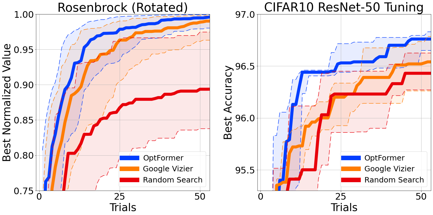
We may now use the OptFormer’s function prediction capability to better guide our imitated policy, similar to techniques found in Bayesian Optimization. Using Thompson Sampling, we may rank our imitated policy’s suggestions and only select the best according to the function predictor. This produces an augmented policy capable of outperforming our industry-grade Bayesian Optimization algorithm in Google Vizier when optimizing classic synthetic benchmark objectives and tuning the learning rate hyperparameters of a standard CIFAR-10 training pipeline.

Left: Best-so-far optimization curve over a classic Rosenbrock function. Right: Best-so-far optimization curve over hyperparameters for training a ResNet-50 on CIFAR-10 via init2winit. Both cases use 10 seeds per curve, and error bars at 25th and 75th percentiles.

Conclusion
Throughout this work, we discovered some useful and previously unknown optimization capabilities of the Transformer. In the future, we hope to pave the way for a universal hyperparameter and blackbox optimization interface to use both numerical and textual data to facilitate optimization over complex search spaces, and integrate the OptFormer with the rest of the Transformer ecosystem (e.g. language, vision, code) by leveraging Google’s vast collection of offline AutoML data.

Acknowledgements
The following members of DeepMind and the Google Research Brain Team conducted this research: Yutian Chen, Xingyou Song, Chansoo Lee, Zi Wang, Qiuyi Zhang, David Dohan, Kazuya Kawakami, Greg Kochanski, Arnaud Doucet, Marc'aurelio Ranzato, Sagi Perel, and Nando de Freitas.

We would like to also thank Chris Dyer, Luke Metz, Kevin Murphy, Yannis Assael, Frank Hutter, and Esteban Real for providing valuable feedback, and further thank Sebastian Pineda Arango, Christof Angermueller, and Zachary Nado for technical discussions on benchmarks. In addition, we thank Daniel Golovin, Daiyi Peng, Yingjie Miao, Jack Parker-Holder, Jie Tan, Lucio Dery, and Aleksandra Faust for multiple useful conversations.

Finally, we thank Tom Small for designing the animation for this post.

Source: Google AI Blog


Towards Helpful Robots: Grounding Language in Robotic Affordances

Over the last several years, we have seen significant progress in applying machine learning to robotics. However, robotic systems today are capable of executing only very short, hard-coded commands, such as “Pick up an apple,” because they tend to perform best with clear tasks and rewards. They struggle with learning to perform long-horizon tasks and reasoning about abstract goals, such as a user prompt like “I just worked out, can you get me a healthy snack?”

Meanwhile, recent progress in training language models (LMs) has led to systems that can perform a wide range of language understanding and generation tasks with impressive results. However, these language models are inherently not grounded in the physical world due to the nature of their training process: a language model generally does not interact with its environment nor observe the outcome of its responses. This can result in it generating instructions that may be illogical, impractical or unsafe for a robot to complete in a physical context. For example, when prompted with “I spilled my drink, can you help?” the language model GPT-3 responds with “You could try using a vacuum cleaner,” a suggestion that may be unsafe or impossible for the robot to execute. When asking the FLAN language model the same question, it apologizes for the spill with "I'm sorry, I didn't mean to spill it,” which is not a very useful response. Therefore, we asked ourselves, is there an effective way to combine advanced language models with robot learning algorithms to leverage the benefits of both?

In “Do As I Can, Not As I Say: Grounding Language in Robotic Affordances”, we present a novel approach, developed in partnership with Everyday Robots, that leverages advanced language model knowledge to enable a physical agent, such as a robot, to follow high-level textual instructions for physically-grounded tasks, while grounding the language model in tasks that are feasible within a specific real-world context. We evaluate our method, which we call PaLM-SayCan, by placing robots in a real kitchen setting and giving them tasks expressed in natural language. We observe highly interpretable results for temporally-extended complex and abstract tasks, like “I just worked out, please bring me a snack and a drink to recover.” Specifically, we demonstrate that grounding the language model in the real world nearly halves errors over non-grounded baselines. We are also excited to release a robot simulation setup where the research community can test this approach.

With PaLM-SayCan, the robot acts as the language model’s “hands and eyes,” while the language model supplies high-level semantic knowledge about the task.

A Dialog Between User and Robot, Facilitated by the Language Model
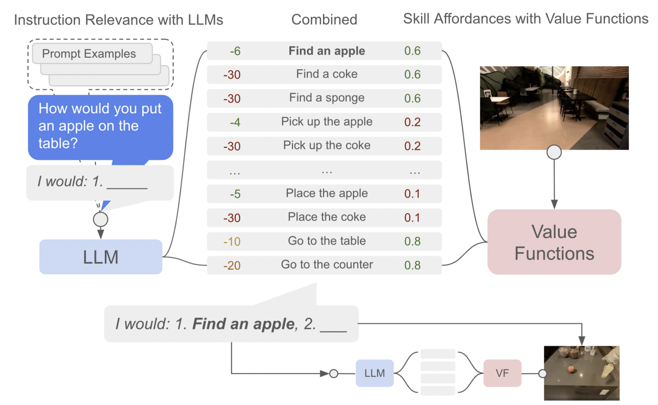
Our approach uses the knowledge contained in language models (Say) to determine and score actions that are useful towards high-level instructions. It also uses an affordance function (Can) that enables real-world-grounding and determines which actions are possible to execute in a given environment. Using the the PaLM language model, we call this PaLM-SayCan.

Our approach selects skills based on what the language model scores as useful to the high level instruction and what the affordance model scores as possible.

Our system can be seen as a dialog between the user and robot, facilitated by the language model. The user starts by giving an instruction that the language model turns into a sequence of steps for the robot to execute. This sequence is filtered using the robot’s skillset to determine the most feasible plan given its current state and environment. The model determines the probability of a specific skill successfully making progress toward completing the instruction by multiplying two probabilities: (1) task-grounding (i.e., a skill language description) and (2) world-grounding (i.e., skill feasibility in the current state).

There are additional benefits of our approach in terms of its safety and interpretability. First, by allowing the LM to score different options rather than generate the most likely output, we effectively constrain the LM to only output one of the pre-selected responses. In addition, the user can easily understand the decision making process by looking at the separate language and affordance scores, rather than a single output.

PaLM-SayCan is also interpretable: at each step, we can see the top options it considers based on their language score (blue), affordance score (red), and combined score (green).

Training Policies and Value Functions
Each skill in the agent’s skillset is defined as a policy with a short language description (e.g., “pick up the can”), represented as embeddings, and an affordance function that indicates the probability of completing the skill from the robot’s current state. To learn the affordance functions, we use sparse reward functions set to 1.0 for a successful execution, and 0.0 otherwise.

We use image-based behavioral cloning (BC) to train the language-conditioned policies and temporal-difference-based (TD) reinforcement learning (RL) to train the value functions. To train the policies, we collected data from 68,000 demos performed by 10 robots over 11 months and added 12,000 successful episodes, filtered from a set of autonomous episodes of learned policies. We then learned the language conditioned value functions using MT-Opt in the Everyday Robots simulator. The simulator complements our real robot fleet with a simulated version of the skills and environment, which is transformed using RetinaGAN to reduce the simulation-to-real gap. We bootstrapped simulation policies’ performance by using demonstrations to provide initial successes, and then continuously improved RL performance with online data collection in simulation.

Given a high-level instruction, our approach combines the probabilities from the language model with the probabilities from the value function (VF) to select the next skill to perform. This process is repeated until the high-level instruction is successfully completed.

Performance on Temporally-Extended, Complex, and Abstract Instructions
To test our approach, we use robots from Everyday Robots paired with PaLM. We place the robots in a kitchen environment containing common objects and evaluate them on 101 instructions to test their performance across various robot and environment states, instruction language complexity and time horizon. Specifically, these instructions were designed to showcase the ambiguity and complexity of language rather than to provide simple, imperative queries, enabling queries such as “I just worked out, how would you bring me a snack and a drink to recover?” instead of “Can you bring me water and an apple?”

We use two metrics to evaluate the system’s performance: (1) the plan success rate, indicating whether the robot chose the right skills for the instruction, and (2) the execution success rate, indicating whether it performed the instruction successfully. We compare two language models, PaLM and FLAN (a smaller language model fine-tuned on instruction answering) with and without the affordance grounding as well as the underlying policies running directly with natural language (Behavioral Cloning in the table below). The results show that the system using PaLM with affordance grounding (PaLM-SayCan) chooses the correct sequence of skills 84% of the time and executes them successfully 74% of the time, reducing errors by 50% compared to FLAN and compared to PaLM without robotic grounding. This is particularly exciting because it represents the first time we can see how an improvement in language models translates to a similar improvement in robotics. This result indicates a potential future where robotics is able to ride the wave of progress that we have been observing in language models, bringing these subfields of research closer together.

Algorithm     Plan     Execute
PaLM-SayCan     84%     74%
PaLM     67%     -
FLAN-SayCan     70%     61%
FLAN     38%     -
Behavioral Cloning     0%     0%
PaLM-SayCan halves errors compared to PaLM without affordances and compared to FLAN over 101 tasks.
SayCan demonstrated successful planning for 84% of the 101 test instructions when combined with PaLM.

If you're interested in learning more about this project from the researchers themselves, please check out the video below:

Conclusion and Future Work
We’re excited about the progress that we’ve seen with PaLM-SayCan, an interpretable and general approach to leveraging knowledge from language models that enables a robot to follow high-level textual instructions to perform physically-grounded tasks. Our experiments on a number of real-world robotic tasks demonstrate the ability to plan and complete long-horizon, abstract, natural language instructions at a high success rate. We believe that PaLM-SayCan’s interpretability allows for safe real-world user interaction with robots. As we explore future directions for this work, we hope to better understand how information gained via the robot’s real-world experience could be leveraged to improve the language model and to what extent natural language is the right ontology for programming robots. We have open-sourced a robot simulation setup, which we hope will provide researchers with a valuable resource for future research that combines robotic learning with advanced language models. The research community can visit the project’s GitHub page and website to learn more.

Acknowledgements
We’d like to thank our coauthors Michael Ahn, Anthony Brohan, Noah Brown, Yevgen Chebotar, Omar Cortes, Byron David, Chelsea Finn, Kelly Fu, Keerthana Gopalakrishnan, Alex Herzog, Daniel Ho, Jasmine Hsu, Julian Ibarz, Alex Irpan, Eric Jang, Rosario Jauregui Ruano, Kyle Jeffrey, Sally Jesmonth, Nikhil J Joshi, Ryan Julian, Dmitry Kalashnikov, Yuheng Kuang, Kuang-Huei Lee, Sergey Levine, Yao Lu, Linda Luu, Carolina Parada, Peter Pastor, Jornell Quiambao, Kanishka Rao, Jarek Rettinghouse, Diego Reyes, Pierre Sermanet, Nicolas Sievers, Clayton Tan, Alexander Toshev, Vincent Vanhoucke, Fei Xia, Ted Xiao, Peng Xu, Sichun Xu, Mengyuan Yan, and Andy Zeng. We’d also like to thank Yunfei Bai, Matt Bennice, Maarten Bosma, Justin Boyd, Bill Byrne, Kendra Byrne, Noah Constant, Pete Florence, Laura Graesser, Rico Jonschkowski, Daniel Kappler, Hugo Larochelle, Benjamin Lee, Adrian Li, Suraj Nair, Krista Reymann, Jeff Seto, Dhruv Shah, Ian Storz, Razvan Surdulescu, and Vincent Zhao for their help and support in various aspects of the project. And we’d like to thank Tom Small for creating many of the animations in this post.

Source: Google AI Blog


Rax: Composable Learning-to-Rank Using JAX

Ranking is a core problem across a variety of domains, such as search engines, recommendation systems, or question answering. As such, researchers often utilize learning-to-rank (LTR), a set of supervised machine learning techniques that optimize for the utility of an entire list of items (rather than a single item at a time). A noticeable recent focus is on combining LTR with deep learning. Existing libraries, most notably TF-Ranking, offer researchers and practitioners the necessary tools to use LTR in their work. However, none of the existing LTR libraries work natively with JAX, a new machine learning framework that provides an extensible system of function transformations that compose: automatic differentiation, JIT-compilation to GPU/TPU devices and more.

Today, we are excited to introduce Rax, a library for LTR in the JAX ecosystem. Rax brings decades of LTR research to the JAX ecosystem, making it possible to apply JAX to a variety of ranking problems and combine ranking techniques with recent advances in deep learning built upon JAX (e.g., T5X). Rax provides state-of-the-art ranking losses, a number of standard ranking metrics, and a set of function transformations to enable ranking metric optimization. All this functionality is provided with a well-documented and easy to use API that will look and feel familiar to JAX users. Please check out our paper for more technical details.

Learning-to-Rank Using Rax
Rax is designed to solve LTR problems. To this end, Rax provides loss and metric functions that operate on batches of lists, not batches of individual data points as is common in other machine learning problems. An example of such a list is the multiple potential results from a search engine query. The figure below illustrates how tools from Rax can be used to train neural networks on ranking tasks. In this example, the green items (B, F) are very relevant, the yellow items (C, E) are somewhat relevant and the red items (A, D) are not relevant. A neural network is used to predict a relevancy score for each item, then these items are sorted by these scores to produce a ranking. A Rax ranking loss incorporates the entire list of scores to optimize the neural network, improving the overall ranking of the items. After several iterations of stochastic gradient descent, the neural network learns to score the items such that the resulting ranking is optimal: relevant items are placed at the top of the list and non-relevant items at the bottom.

Using Rax to optimize a neural network for a ranking task. The green items (B, F) are very relevant, the yellow items (C, E) are somewhat relevant and the red items (A, D) are not relevant.

Approximate Metric Optimization
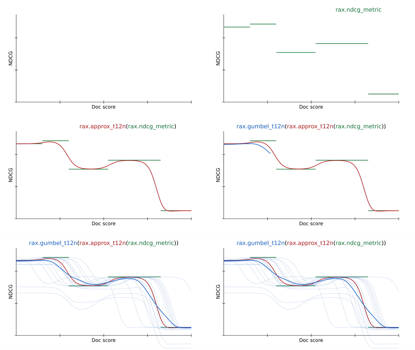
The quality of a ranking is commonly evaluated using ranking metrics, e.g., the normalized discounted cumulative gain (NDCG). An important objective of LTR is to optimize a neural network so that it scores highly on ranking metrics. However, ranking metrics like NDCG can present challenges because they are often discontinuous and flat, so stochastic gradient descent cannot directly be applied to these metrics. Rax provides state-of-the-art approximation techniques that make it possible to produce differentiable surrogates to ranking metrics that permit optimization via gradient descent. The figure below illustrates the use of rax.approx_t12n, a function transformation unique to Rax, which allows for the NDCG metric to be transformed into an approximate and differentiable form.

Using an approximation technique from Rax to transform the NDCG ranking metric into a differentiable and optimizable ranking loss (approx_t12n and gumbel_t12n).

First, notice how the NDCG metric (in green) is flat and discontinuous, making it hard to optimize using stochastic gradient descent. By applying the rax.approx_t12n transformation to the metric, we obtain ApproxNDCG, an approximate metric that is now differentiable with well-defined gradients (in red). However, it potentially has many local optima — points where the loss is locally optimal, but not globally optimal — in which the training process can get stuck. When the loss encounters such a local optimum, training procedures like stochastic gradient descent will have difficulty improving the neural network further.

To overcome this, we can obtain the gumbel-version of ApproxNDCG by using the rax.gumbel_t12n transformation. This gumbel version introduces noise in the ranking scores which causes the loss to sample many different rankings that may incur a non-zero cost (in blue). This stochastic treatment may help the loss escape local optima and often is a better choice when training a neural network on a ranking metric. Rax, by design, allows the approximate and gumbel transformations to be freely used with all metrics that are offered by the library, including metrics with a top-k cutoff value, like recall or precision. In fact, it is even possible to implement your own metrics and transform them to obtain gumbel-approximate versions that permit optimization without any extra effort.

Ranking in the JAX Ecosystem
Rax is designed to integrate well in the JAX ecosystem and we prioritize interoperability with other JAX-based libraries. For example, a common workflow for researchers that use JAX is to use TensorFlow Datasets to load a dataset, Flax to build a neural network, and Optax to optimize the parameters of the network. Each of these libraries composes well with the others and the composition of these tools is what makes working with JAX both flexible and powerful. For researchers and practitioners of ranking systems, the JAX ecosystem was previously missing LTR functionality, and Rax fills this gap by providing a collection of ranking losses and metrics. We have carefully constructed Rax to function natively with standard JAX transformations such as jax.jit and jax.grad and various libraries like Flax and Optax. This means that users can freely use their favorite JAX and Rax tools together.

Ranking with T5
While giant language models such as T5 have shown great performance on natural language tasks, how to leverage ranking losses to improve their performance on ranking tasks, such as search or question answering, is under-explored. With Rax, it is possible to fully tap this potential. Rax is written as a JAX-first library, thus it is easy to integrate it with other JAX libraries. Since T5X is an implementation of T5 in the JAX ecosystem, Rax can work with it seamlessly.

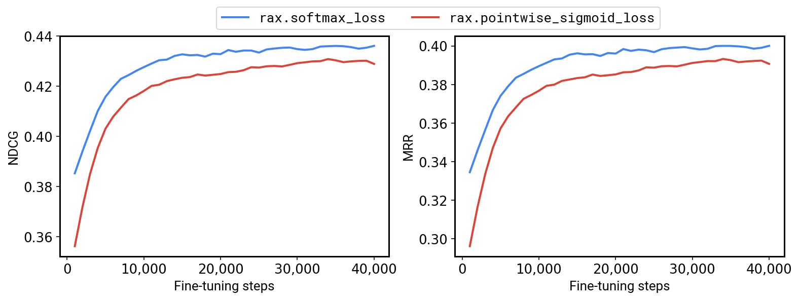
To this end, we have an example that demonstrates how Rax can be used in T5X. By incorporating ranking losses and metrics, it is now possible to fine-tune T5 for ranking problems, and our results indicate that enhancing T5 with ranking losses can offer significant performance improvements. For example, on the MS-MARCO QNA v2.1 benchmark we are able to achieve a +1.2% NDCG and +1.7% MRR by fine-tuning a T5-Base model using the Rax listwise softmax cross-entropy loss instead of a pointwise sigmoid cross-entropy loss.

Fine-tuning a T5-Base model on MS-MARCO QNA v2.1 with a ranking loss (softmax, in blue) versus a non-ranking loss (pointwise sigmoid, in red).

Conclusion
Overall, Rax is a new addition to the growing ecosystem of JAX libraries. Rax is entirely open source and available to everyone at github.com/google/rax. More technical details can also be found in our paper. We encourage everyone to explore the examples included in the github repository: (1) optimizing a neural network with Flax and Optax, (2) comparing different approximate metric optimization techniques, and (3) how to integrate Rax with T5X.

Acknowledgements
Many collaborators within Google made this project possible: Xuanhui Wang, Zhen Qin, Le Yan, Rama Kumar Pasumarthi, Michael Bendersky, Marc Najork, Fernando Diaz, Ryan Doherty, Afroz Mohiuddin, and Samer Hassan.

Source: Google AI Blog


Efficient Video-Text Learning with Iterative Co-tokenization

Video is an ubiquitous source of media content that touches on many aspects of people’s day-to-day lives. Increasingly, real-world video applications, such as video captioning, video content analysis, and video question-answering (VideoQA), rely on models that can connect video content with text or natural language. VideoQA is particularly challenging, however, as it requires grasping both semantic information, such as objects in a scene, as well as temporal information, e.g., how things move and interact, both of which must be taken in the context of a natural-language question that holds specific intent. In addition, because videos have many frames, processing all of them to learn spatio-temporal information can be computationally expensive. Nonetheless, understanding all this information enables models to answer complex questions — for example, in the video below, a question about the second ingredient poured in the bowl requires identifying objects (the ingredients), actions (pouring), and temporal ordering (second).

An example input question for the VideoQA task “What is the second ingredient poured into the bowl?” which requires deeper understanding of both the visual and text inputs. The video is an example from the 50 Salads dataset, used under the Creative Commons license.

To address this, in “Video Question Answering with Iterative Video-Text Co-Tokenization”, we introduce a new approach to video-text learning called iterative co-tokenization, which is able to efficiently fuse spatial, temporal and language information for VideoQA. This approach is multi-stream, processing different scale videos with independent backbone models for each to produce video representations that capture different features, e.g., those of high spatial resolution or long temporal durations. The model then applies the co-tokenization module to learn efficient representations from fusing the video streams with the text. This model is highly efficient, using only 67 giga-FLOPs (GFLOPs), which is at least 50% fewer than previous approaches, while giving better performance than alternative state-of-the-art models.

Video-Text Iterative Co-tokenization
The main goal of the model is to produce features from both videos and text (i.e., the user question), jointly allowing their corresponding inputs to interact. A second goal is to do so in an efficient manner, which is highly important for videos since they contain tens to hundreds of frames as input.

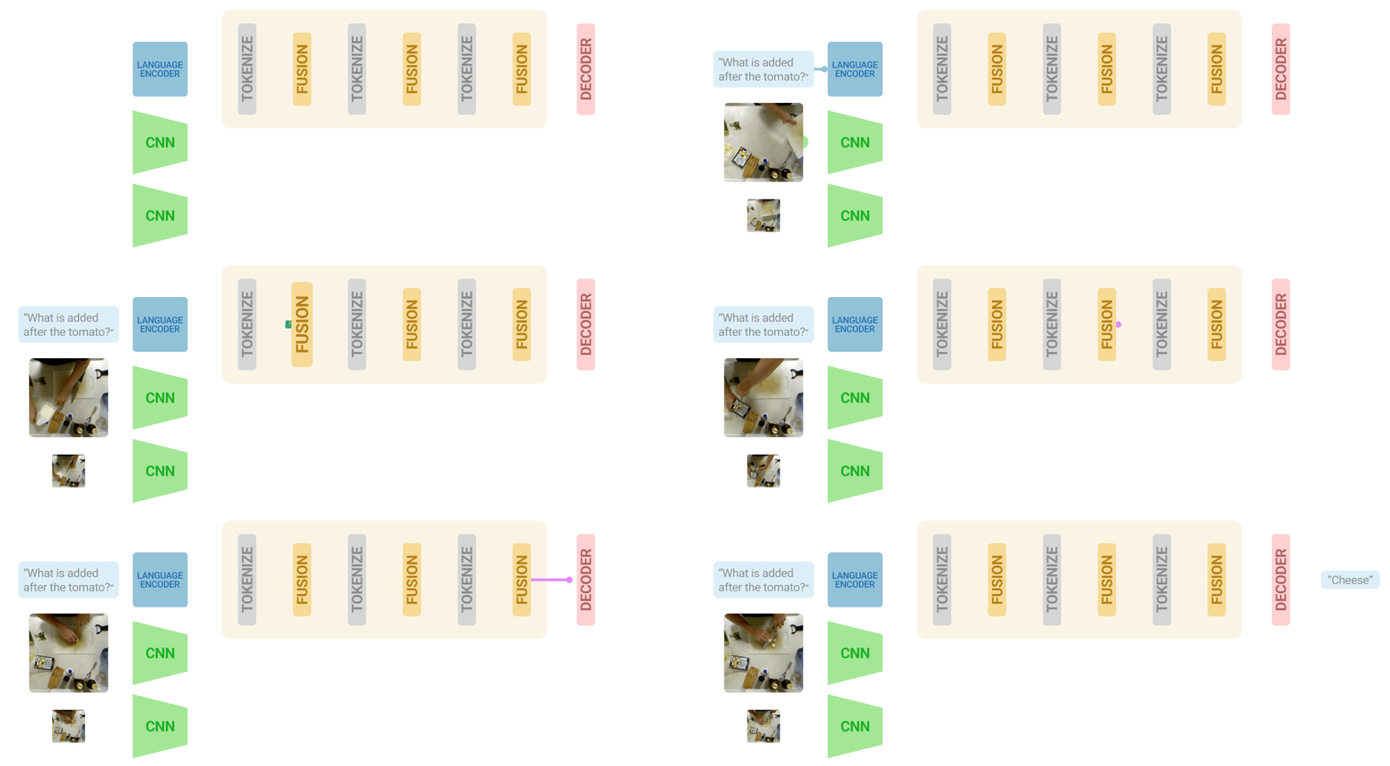
The model learns to tokenize the joint video-language inputs into a smaller set of tokens that jointly and efficiently represent both modalities. When tokenizing, we use both modalities to produce a joint compact representation, which is fed to a transformer layer to produce the next level representation. A challenge here, which is also typical in cross-modal learning, is that often the video frame does not correspond directly to the associated text. We address this by adding two learnable linear layers which unify the visual and text feature dimensions before tokenization. This way we enable both video and text to condition how video tokens are learned.

Moreover, a single tokenization step does not allow for further interaction between the two modalities. For that, we use this new feature representation to interact with the video input features and produce another set of tokenized features, which are then fed into the next transformer layer. This iterative process allows the creation of new features, or tokens, which represent a continual refinement of the joint representation from both modalities. At the last step the features are input to a decoder that generates the text output.

As customarily done for VideoQA, we pre-train the model before fine-tuning it on the individual VideoQA datasets. In this work we use the videos automatically annotated with text based on speech recognition, using the HowTo100M dataset instead of pre-training on a large VideoQA dataset. This weaker pre-training data still enables our model to learn video-text features.

Visualization of the video-text iterative co-tokenization approach. Multi-stream video inputs, which are versions of the same video input (e.g., a high resolution, low frame-rate video and a low resolution, high frame-rate video), are efficiently fused together with the text input to produce a text-based answer by the decoder. Instead of processing the inputs directly, the video-text iterative co-tokenization model learns a reduced number of useful tokens from the fused video-language inputs. This process is done iteratively, allowing the current feature tokenization to affect the selection of tokens at the next iteration, thus refining the selection.

Efficient Video Question-Answering
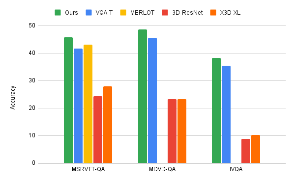
We apply the video-language iterative co-tokenization algorithm to three main VideoQA benchmarks, MSRVTT-QA, MSVD-QA and IVQA, and demonstrate that this approach achieves better results than other state-of-the-art models, while having a modest size. Furthermore, iterative co-tokenization learning yields significant compute savings for video-text learning tasks. The method uses only 67 giga-FLOPs (GFLOPS), which is one sixth the 360 GFLOPS needed when using the popular 3D-ResNet video model jointly with text and is more than twice as efficient as the X3D model. This is all the while producing highly accurate results, outperforming state-of-the-art methods.

Comparison of our iterative co-tokenization approach to previous methods such as MERLOT and VQA-T, as well as, baselines using single ResNet-3D or X3D-XL.

Multi-stream Video Inputs
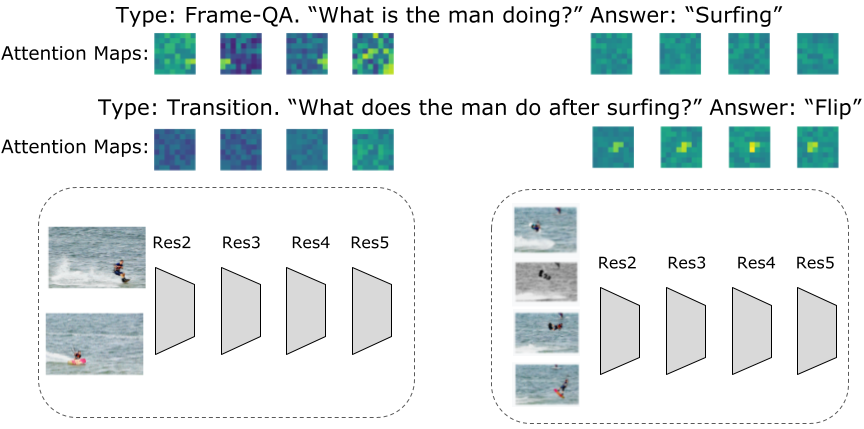
For VideoQA, or any of a number of other tasks that involve video inputs, we find that multi-stream input is important to more accurately answer questions about both spatial and temporal relationships. Our approach utilizes three video streams at different resolutions and frame-rates: a low-resolution high frame-rate, input video stream (with 32 frames-per-second and spatial resolution 64x64, which we denote as 32x64x64); a high-resolution, low frame-rate video (8x224x224); and one in-between (16x112x112). Despite the apparently more voluminous information to process with three streams, we obtain very efficient models due to the iterative co-tokenization approach. At the same time these additional streams allow extraction of the most pertinent information. For example, as shown in the figure below, questions related to a specific activity in time will produce higher activations in the smaller resolution but high frame-rate video input, whereas questions related to the general activity can be answered from the high resolution input with very few frames. Another benefit of this algorithm is that the tokenization changes depending on the questions asked.

Visualization of the attention maps learned per layer during the video-text co-tokenization. The attention maps differ depending on the question asked for the same video. For example, if the question is related to the general activity (e.g., surfing in the figure above), then the attention maps of the higher resolution low frame-rate inputs are more active and seem to consider more global information. Whereas if the question is more specific, e.g., asking about what happens after an event, the feature maps are more localized and tend to be active in the high frame-rate video input. Furthermore, we see that the low-resolution, high-frame rate video inputs provide more information related to activities in the video.

Conclusion
We present a new approach to video-language learning that focuses on joint learning across video-text modalities. We address the important and challenging task of video question-answering. Our approach is both highly efficient and accurate, outperforming current state-of-the-art models, despite being more efficient. Our approach results in modest model sizes and can gain further improvements with larger models and data. We hope this work provokes more research in vision-language learning to enable more seamless interaction with vision-based media.

Acknowledgements
This work is conducted by AJ Pierviovanni, Kairo Morton, Weicheng Kuo, Michael Ryoo and Anelia Angelova. We thank our collaborators in this research, and Soravit Changpinyo for valuable comments and suggestions, and Claire Cui for suggestions and support. We also thank Tom Small for visualizations.

Source: Google AI Blog